City, University of London Institutional Repository
Citation
: Driver, C., Trapani, L. and Urga, G. (2013). On the use of cross-sectional
measures of forecast uncertainty. International Journal of Forecasting, 29(3), pp. 367-377.
doi: 10.1016/j.ijforecast.2012.11.005
This is the accepted version of the paper.
This version of the publication may differ from the final published
version.
Permanent repository link:
http://openaccess.city.ac.uk/4873/
Link to published version
: http://dx.doi.org/10.1016/j.ijforecast.2012.11.005
Copyright and reuse:
City Research Online aims to make research
outputs of City, University of London available to a wider audience.
Copyright and Moral Rights remain with the author(s) and/or copyright
holders. URLs from City Research Online may be freely distributed and
linked to.
City Research Online:
http://openaccess.city.ac.uk/
[email protected]
On the Use of Cross-Sectional Measures of
Forecast Uncertainty
Ciaran Driver
(School of Oriental and African Studies, UK)
Lorenzo Trapani
(Cass Business School, UK)
Giovanni Urga
(Cass Business School, UK, and University of Bergamo, Italy)
On the Use of Cross-Sectional Measures of Uncertainty
Abstract. This paper investigates the role of cross sectional dependence among private
forecasters, assessing its impact on measuring and using forecasting uncertainty. We study un-der which circumstances cross sectional measures of uncertainty (such as disagreement across forecasters) are valid proxies for private information, analysing the impact of distributional as-sumptions on private signals. In particular, we explore the role played by cross dependence among forecasters, arising e.g. from partially shared private information. We validate the theory through a Monte Carlo exercise, which reinforces our …ndings, and through an application to US nonfarm payroll data.
J.E.L. Classi…cation Numbers: C21, C22.
1
Introduction
The main question of this paper is: can disagreement among private forecasters (irrespective of its determinants) be used to improve predictive ability? We base our analysis on the same setup as in Engle (1983), using a simple model in which an outcome variable,yt, has DGP determined
by its past value(s) and some other explanatory variables, which may be observable or not. In this context,ytis predicted by a researcher by using only past information. This can be due to
the other explanatory variables being unobservable, or to the model (s)he employs simply not including them. As well as by the researcher,yt may be predicted by several individuals, who
use the publicly available past information on yt and some other explanatory variables. Such
variables may be available only to them; alternatively, the variable may be observable but only used by some forecasters. Based on this framework, we propose that the researcher, in addition to using standard proxies such as the mean of the individual forecasts, should proxy the unavailable explanatory variables by using a measure of dispersion among the individual forecasters. The most obvious measure of dispersion is the cross sectional variance (henceforth de…ned asCSt(2)), which is traditionally used as a measure of disagreement (see e.g. Giordani and Soderlind, 2003). We show that using CSt(2) as a regressor in a model for yt can increase forecasting ability by
reducing the Mean Squared Error (MSE) of forecasts. However, we also show that the usefulness ofCSt(2) is very sensitive to the distributional features of the explanatory variables in the DGP of yt. Indeed, as a leading counterexample we show that augmenting an ARMA speci…cation
for yt by including CS(2)t yields no gain in predictive ability when the omitted explanatory
variables follow a normal distribution. In order to generalise this, we also consider a generalised version of cross sectional disagreement, calledCS(tk), which, in essence, is based on representing cross sectional dispersion as thek-th sample moment of individual forecasts. Such generalised measures are not sensitive to the distribution of the omitted variables. Given that the CS(tk)s are non structural in nature, the approach that we recommend is a General-to-Speci…c (GETS) approach based on using the AutoMetrics option on OxMetrics 6.2 (Doornik, 2009; Castle et al., 2011), …tting an ADL model toyt using theCSt(k)s, and their lags.
We show that the CSt(k)s manage to proxy the extra omitted variables by exploiting the presence of cross dependence among them. This has a twofold implication. On the one hand, cross dependence among the information sets available to individual forecasters is necessary in order for the CSt(k)s to improve forecasting ability. On the other hand, the reverse argument holds: whenever there are cross dependent forecasts, even in presence of unobservable, private information, it is possible to proxy such private information by using disagreement, and use it to better predictyt. Individual forecasts that are correlated have been noted in various contexts.
on the presence of correlation in the Survey of Professional Forecasters in Elliott (2011), and the theoretical framework therein, where the impact of cross correlation in determining the optimal forecast is discussed. Thus, cross dependence among forecasters is an important feature in em-pirical studies. Several theoretical explanations have been proposed, from presence of partially shared private information (Patton and Timmermann, 2010) to herding (Scharfstein and Stein, 1990; Stein, 2003).
As well as the contribution above, we review the relationship between the traditionally em-ployed measure of cross sectional dispersion CS(2)t , and GARCH-type measures. As mentioned above, this is a “classical” investigation (see Lahiri and Sheng, 2010); in our context, we assess the impact of cross dependence on this relationship, showing that it leads to an ambiguous sign in the di¤erence between them.
The paper is organised as follows. We …rst (Section 2) introduce theCSt(k)s, showing how they
can reduce the forecast error foryt. This is validated through a Monte Carlo exercise and through
the application to the prediction of the United States Non-farm Payroll index (NFP henceforth) - Section 3. Section 4 concludes. All proofs and derivations are in the supplementary online material.
2
Use of cross section uncertainty in forecasting
The starting point of our analysis is equation (9) in Engle (1983, p. 295):
yt= yt 1+ 0t"t+ t; (1)
with j j<1. Equation (1) states that yt is generated by a process which depends on its past
value(s), and on a set of n explanatory variables, "t ["1t; :::; "nt]0; this could be regarded as
“the reduced form of a structural model” (Engle, 1983, p. 295), with t being the error term. As far as forecastingytis concerned, we start our analysis from the same viewpoint as Engle: yt
is predicted by a researcher who has onlyyt 1 at his/her disposal. Thus, the researcher predicts
yt as
yrt = yt 1:
Hence, the forecast error in this case is yt yrt = 0t"t + t. In this respect, (1), from the
researcher’s viewpoint, is a model with latent explanatory variables (the"its). The researcher’s
model is
yt= yt 1+vt; (2)
wherevt= t+ 0t"t. Thus, from the researcher’s viewpoint, using (2) instead of (1) is an omitted
variables problem.
Alongside the researcher, Engle’s framework postulates the existence ofnforecasters, each of whom has inside information on his/her own"it; in this respect,"it is customarily interpreted
forecasters uses in order to predictyt. This entails that thei-th forecaster predictsyt as
yit= yt 1+ it"it: (3)
Equation (3) is based on the assumption that and it are observable, and therefore it may
be viewed as an infeasible prediction. We use this as our baseline case. In the comments to Proposition 1 below, we analyse the impact of having to estimate both and it on the
predictionyi t.
We consider the following assumptions.
Assumption 1: tand"tare mutually independent, zero mean, covariance stationary processes
withE(yt 1 t) = 0, E(yt 1"t) = 0, V ar( t) = 2 <1and E("it"jt) = !ij with!ij = 1 for
alli=j.
Assumption 2: the its are non-stochastic quantities that satisfy(i) 0t"t =Op(1), (ii) 0<
0
tE("t"0t) t < 1 as n ! 1 for all t; (iii) 0 < Pni=1 2it"it2 < 1 as n ! 1 for all t; (iv)
Eh( 0t"t)4
i
<1andEh Pni=1 2it"2it 2i<1asn! 1;(v)k tk=O(1)for allnandt.
Assumption 1 considers the presence of contemporaneous correlation, and therefore of inter-actions among agents. As pointed out above, from the researcher’s viewpoint, using (2) instead of (1) is an omitted variables problem; assumingE[yt 1"t] = 0 entails that this does not cause
inconsistency of the estimated .
Assumption 2 allows the its to be time dependent; this also entails that the number of
forecasters,n, is allowed to vary over time, as it is typical in empirical applications. In addition to this, Assumption 2 poses some restrictions on the moments of 0t"t as n ! 1. The square
summability condition prevents the variance of the error term in regression (1) from exploding as the number of individuals grows; a similar assumption is contained in Pesaran and Weale (2006).
The regressors "it are not observable to the researcher. Thus, (s)he could proxy them using
some variables that are related to them. In order to construct such an “instrument”, recall that each individual forecaster predictsytusingyt 1 and"it. Thei-th forecaster’s prediction error is
given by
"it yt yit= t+
X
j6=i
jt"jt: (4)
De…neCSt(2) as the dispersion of the individual predictions around their mean
CSt(2) =
n
X
i=1
yit yt
2
=
n
X
i=1 2
it"2it
1
n(
0
t"t)2; (5)
where the second equality follows fromyi
t yt=yit n1
Pn
Equation (5) illustrates how CSt(2) can be used by the researcher as a proxy for the "its.
The quantity CSt(2) contains the squares of the "its, and it is observable at time t, since it is
constructed using predictions for yt which are available prior to t. From a technical point of
view, our de…nition ofCSt(2) is di¤erent from the one usually employed in the literature, where cross sectional dispersion is de…ned as 1
n
Pn
i=1 yti yt
2
. In our case, there is no need to divide byn, since Pni=1 yti yt
2
is already normalised by assuming that the its are summable. In
order to make the two measures comparable, further assumptions are needed on the its, e.g.
that they sum to one.
Since CSt(2) contains a transformation of the"its, in order to reduce the error term in (2),
i.e. vt= t+ 0t"t, the econometrician could employ the augmented regression:
yt= yt 1+ CSt(2)+vt; (6)
where
vt =vt( ) = t+ 0t"t CSt(2):
Considering an MSE criterion, using CSt(2) improves the prediction of yt in (2) as long as
E v 2
t < E v2t . Particularly, for the case of an estimator that minimizesE vt2 , the model
improves after addingCSt(2) if 6= 0(otherwise there is only an unnecessary reduction in the degree of freedom) and if, for the chosen value of (say ), E v 2
t is indeed smaller than
E v2
t .
It holds that:
Proposition 1 Let Assumptions 1-2 hold withEk"tk4<1and consider
minE[vt( )]2: (7)
This has solution
=
n2E 0"
tPni=1 2it"2it nE
h ( 0
t"t)3
i
Eh( 0
t"t)2 n(Pni=1 2it"2it)
i2 (8)
=
EhCSt(2)( 0 t"t)
i
E CSt(2) 2
:
Also, it holds thatE[vt( )]2 E vt2 , withE[vt( )]2 =E v2t if and only if = 0. The same result holds asn! 1, assuming that supiEj"itj4<1andsupij itj=O n 1=4 .
usingCSt(2), which contains (a quadratic transformation of) the"its; improvements are present
when 6= 0.
It is interesting to explore what happens when the number of forecasters or alternative models,
n, passes to in…nity. Asn! 1, Assumption 2 ensures that 0
t"tandPni=1 2it"2itdo not vanish.
Thus,CSt(2)=Pni=1 2
it"2it+Op n 1 . From (8), this entails that =Op(1).
Building on the calculations in the supplementary material, it can be shown that
E[vt( )]2 E v2t = 2E
2 4
n
X
i=1 2
it"2it
!23
5 2 E
"
0 t"t
n
X
i=1 2
it"2it
#
+Op
1
n +Op
1
n2 :
Thus, it follows from (8) that
E[vt( )]2 E v2t =
h
E CSt(2) 0
t"t
i2
E CS(2)t 2
;
which is always negative as long asE CSt(2) 0
t"t 6= 0. Therefore, asn ! 1, there is still a
gain in forecasting accuracy.
From a technical point of view, the main result in Proposition 1 (i.e., the possibility of prox-ying private information throughCSt(2)) holds under more general conditions than Assumptions 1 and 2. For example, if we assumed that"tand tare not independent, equation (8) would be
modi…ed into = E
h
CS(2)t ( 0t"t t)
i
Eh CSt(2)
i - this follows from the same algebra as in the proof of the Proposition. Even in this case, is not, in general, equal to zero, and thus it can be employed as a proxy for the"its.
It is worth pointing out that the result in Proposition 1 are based on the assumption that the
i-th forecaster knows and uses the actual values of and i (we suppress the dependence onifor
simplicity). As it can be expected, Proposition 1 does not change if and i are replaced with
consistent estimators in (3). The i-th forecaster would estimate and i from his/her model,
viz.
yit= yt 1+ i"it+vti; (9)
with vi
t = t+
P
j6=i"it. In view of (1), this is an omitted variables problem, similarly to the
one observed for the researcher when using (2). Indeed, estimating consistently is possible for the i-th forecaster, due to the independence between yt 1 and the omitted "its. However,
consistent estimation of ifrom (9) is fraught with di¢ culties. Of course, if the"its are assumed
to be uncorrelated (as in Engle, 1983), then i can be estimated applying e.g. OLS to (9) and
the estimate can be expected to be consistent. Conversely, if the"its are correlated, consistency
show that even using inconsistently estimated is does not make CSt(2) useless. Consider (9),
and, for simplicity, let = 0and assume that"it is normalised so thatPTt=1"2it=T. The OLS
estimation error of i is
^i i=
1
T
T
X
t=1
"it t+X
j6=i j
1
T
T
X
t=1
"it"jt
!
=I+II:
ConsideringI, this isOp T 1=2 under Assumption 1. Turning toII, the only way in which^i
can be consistent is ifPj6=i j T 1PTt=1"it"jt =op(1). Using the notation in Assumption 1
and a LLN, this could be rewritten asPj6=i j!ij =op(1). This holds e.g. if !ij =O(T )for
some >0 for all j 6=i, but this may be a rather arti…cial requirement. Thus, in general, ^i
is estimated inconsistently when using (9), which is not surprising due to the omitted variable problem mentioned above. From the researcher’s point of view, this entails that CSt(2) should be replaced by its empirical counterpart, saydCS(2)t , de…ned as
d
CS(2)t = n
X
i=1
yit yt
2 =
n
X
i=1 ^2i"2it
1
n ^
0" t
2
;
so that (6) becomes
yt= yt 1+ dCS
(2)
t + ^vt;
withv^t = ^vt( ) = t + 0
t"t dCS
(2)
t . However, following the same passages as in the proof
of Proposition 1, it can be shown that the solution to the minimisation problemmin E[^vt( )]2 is
(
E
" d
CS(2)t
2#) 1
E dCS(2)t ( 0"
t) , which is not, in general, equal to zero. Thus, from the
researcher’s point of view, usingCSd(2)t does not, in general, cause problems, even if the is (or
some of them) are not estimated consistently. The intuition behind this is that the estimation error ^i i may not vanish asT ! 1, but its asymptotic bias contains the "jts (withj 6=i),
which is indeed useful information. From an empirical point of view, of course the researcher does not know how the is have been estimated, and therefore the only way of assessing whether
usingdCS(2)t is useful is to estimate (6) and check whether is signi…cantly di¤erent from zero. Finally, note that equation (8) also illustrates some potential issues with using CSt(2): in general, the usefulness ofCSt(2)(and ofdCS
(2)
t ) depends in a non-trivial way on the (unobservable)
distributional properties of the "its. In order to illustrate this, we consider, as an example, the
case of the "its being Gaussian; assuming normality of private signals is a typical assumption
in the literature (see e.g. the literature on herding: Chamley, 2004). In such case, it holds that = 0, and therefore CSt(2) is not useful. This is due to the fact that in the numerator of (8) there are quantities likeE "3it and E "2it"jt with i6=j, which are all equal to zero if
"it is Gaussian. This is only an illustrative example, based on the infeasible i-th prediction yti
assumptions to analyse in which casesCS(2)t can be employed.
In order to expand the framework and to make it robust to the distributional properties of
the"its, we introduce a generalised class of measures of cross sectional disagreement. De…ne the
k-th sample moment of the individual forecasts:
CSt(k) = n
X
i=1
yit yt k
(10)
=
n
X
i=1 1
n
0
t"t it"it k
=
n
X
i=1
k
X
j=0 1
nk j
k
j (
0 t"t)
k j j it"
j it;
fork= 2; :::; p, where the last equality comes from Pascal’s triangle.
The de…nition of CSt(k) is based on the case of …nite n. However, as n ! 1, it is pos-sible to envisage that Pni=1 1n 0t"t it"it
k
converges to zero. Indeed, using theCr
inequal-ity, Pni=1 n1 0
t"t it"it k
Cn1 k( 0
t"t)k + CPni=1 kit"kit. Assumption 2(i) stipulates that
n1 k( 0
t"t)k = Op n1 k . The argument for Pni=1 kit"kit is subtler, but again in light of
As-sumption 2(i), it is natural to think of the case of it being proportional to n 1=2 (albeit non
necessary; the assumption allows for greater ‡exibility). In such case, Pni=1 k
it"kit would also
vanish asn! 1, at a rateO n1 k2 , provided that Ej"itjk <1. In light of this, we propose
to modifyCSt(k)as
CS(tk)=nk2 1CS (k)
t : (11)
It can be expected that, asn! 1,CSt(k) converges to( 1) k
limn!1 Pni=1 kitE "kit .
Let = 2; :::; p 0 andgCSt=
h
CSt(2); :::; CS
(p)
t
i0
. The following Assumption, which com-plements Assumption 2, summarizes the discussion above.
Assumption 3: for all n it holds that (i) E ( 0
t"t)p <1 and 0 < n
p
2 1Pn
i=1E h
( pit"pit)2i
<1and(ii) E gCStgCS 0
t is positive de…nite.
Based on the discussion above, equation (2) could be augmented as
yt = yt 1+
p
X
k=2
kCS
(k)
t +vt
= yt 1+ 0gCSt+vt: (12)
Similarly to Proposition 1, it holds that:
Theorem 1 Let Assumptions 1-3 hold withEk"tk2p<1and consider
This has solution
=hE gCStgCS 0 t
i 1h
E gCSt 0t"t
i
:
Also, it holds that E[vt( )]2 E v2
t , withE[vt( )]
2
=E v2
t if and only if = 0. The
same result holds asn! 1, assuming that supiEj"itj2p<1andsupij itj=O n 1=4 .
Theorem 1 is similar to Proposition 1. Particularly, gains are present if at least one element of is non-zero, i.e. if at least one element ofE CSgt 0t"t is non-zero, viz.
k
X
j=0 1
nk j
k
j E
" ( 0t"t)
k jXn i=1
j it"
j it
#
6
= 0;
for some k. Of course, in order to use this approach one needs the further assumption that
Ek"tk2p <1. However, in this case, the MSE could be further reduced. Similarly to Proposition
1, in general thei-th forecaster is not able to use the true values of and i. From the researcher’s
point of view, this entails that theCSt(k)s are computed based on possibly inconsistent estimates of the is. Even in this case, this is not necessarily a problem for the researcher, and using the
CSt(k)s can still help improve the prediction ofyt.
Another advantage of using theCSt(k)s is that the dimensionality of the estimation problem is reduced. Indeed, if one were to estimate the its in equation (1), even assuming homogeneity
over time (i.e. it = i for all t), as n ! 1 this would be a classical incidental parameters
problem (Neyman and Scott, 1948). Conversely, consider the OLS estimator of , say^, in the regression yt = yt 1+ 0gCSt+vt. Under the martingale di¤erence assumption for the "its,
T 1P
tgCStyt 1 =Op T 1=2 and thus ^ = +Op T 1=2 .
Finally, it is interesting to note that the is need not represent di¤erent individuals. As a possible, alternative example, the equationyti= yt 1+ it"itcould be the prediction generated
from modeli(which augments the AR(1) model by using a set of regressors"it) out ofnpossible
models. In this case, Proposition 1 and Theorem 1 provide guidelines as to how to combine forecasts, as well as (see remarks above) spelling out the distributional assumptions on the regressors"it that make the combined forecast better than the basic AR(1) model.
The results in Proposition 1 and in Theorem 1 illustrate how measures of forecast disagree-ment can help to improve the forecast of yt, especially under the realistic case of presence of
cross dependence.
3
Applications
yield better forecasts for yt, using synthetic data. Secondly, we validate our …ndings with an
application to US NFP data.
3.1
Monte Carlo simulations
The design of our experiments is as follows. We generate T + 1000 datapoints (discarding the …rst1000 to avoid dependence on initial conditions) for yt using equation (2). The alternative
sample sizes we use areT 2 f50;100;200g. Also, we set in (2) equal to0:5; this value is chosen based on the actual …rst order partial autocorrelation in the dataset used in Section 3.2. Other unreported results show that changing has virtually no impact on the results. As far as the number of forecasters is concerned, we setn2 f15;20;25;30;45;60;80g.
We generate tas i.i.d. normal with zero mean and variance 2 = 1(this parameter, too, does not appear to have much impact). We draw the its fromiidN n 1=2;1 , so that Assumption
2 is satis…ed; cross dependence among the"its is modelled by setting, fori6=j,E("it"jt) =!2
f0;0:2;0:4;0:6;0:8;0:99g.
The impact of asymmetry and cross dependence in the distribution of the"its is analysed by
generating them as (centered and scaled) chi-squared withp degrees of freedom. Experiments are carried out withp=f1;5;10;30;50g. As a benchmark, we also report an experiment where
"it N(0;1) - according to the theory, there should be no gain at all in this case when using
CSt(2). We also consider using theCSt(k)s when"it N(0;1). In particular, we proceed in the
following way. We includeCS(2)t andCSt(3) only forT = 50, in order not to saturate the degree of freedom. When T = 100, we addCSt(5) andCSt(6) (as well asCSt(2) and CS(3)t ); …nally, we consider CSt(2) up to CS
(8)
t in the case T = 200. In these cases, Theorem 1 states that there
should be some gains in predictive ability.
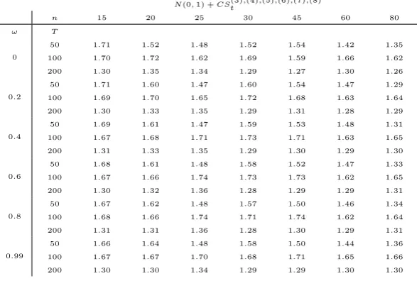
We measure the gain in predictive ability by using in-sample forecasts for all t = 1; :::; T. LetM SE1andM SE2 be the Mean Squared Errors from models (2) and (12) respectively. The values in Table 1 are calculated as
gain= M SE2 M SE1
M SE1
: (13)
The number of replications is10;000.
[Insert Table 1 somewhere here]
The results complement Proposition 1 and Theorem 1. Aspincreases, the distribution of the
"its approaches a Gaussian distribution; as a consequence, gains become increasingly smaller.
Also, gains monotonically decrease as!, the degree of cross-dependence, decreases.
As predicted by the theory, in the case of Gaussian"it, there are no improvements in predictive
theCSt(k)s seems to yield some reduction in the MSE, in contrast to the case of Gaussian signals
withCSt(2)as a proxy; larger sample sizes, which allow for higher orderCSt(k)s, show a moderate improvement in predictive ability. It is interesting to explore the link between the chi-squared and the Gaussian case. When p is as large as 30, and there is no cross dependence (! = 0), there is no gain from adding CSt(2). This follows from the theory: as p ! 1, the Central Limit Theorem entails that the distribution of "it is tantamount to a normal distribution. In
this case, predictive ability is present when there is a large amount of cross dependence. This is probably due to the fact that, when ! is large, the convergence to the normal distribution gets slower. Table 1 also shows the role played by the number of forecasters n: irrespective of the distributional properties of the private signal "it, increases in n amplify the results, and
particularly the spread between MSE gains when!= 0as opposed to != 0:99.
3.2
Empirical exercise
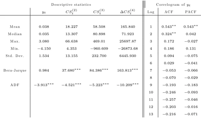
In order to validate the use of the CSt(k)s studied in Proposition 1 and Theorem 1, we report an illustrative application based on predicting a “classical”economic indicator, namely (changes in the) US NFP data (yt). Our monthly dataset spans from June 2000 until July 2004 (thus,
T = 50); the number of forecasters,nt, increases over time, ranging between37 and79 with a
median value of56.
We calculateCSt(k) as de…ned in (11), considering k= 2;3 and 4. Descriptive statistics for all the series are reported in Table 2, where we also report the correlogram foryt. Preliminary
analysis shows that CSt(4) is non-stationary; thus, we use its …rst di¤erence, CS(4)t , whose descriptive statistics are reported in the Table. The correlogram ofytshows a quite clear AR(1)
pattern.
[Insert Table 2 somewhere here]
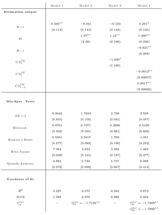
We now turn to analysing the output. We compare the predictive ability of four di¤erent models:
Model 1: yt= + yt 1+vt;
Model 2: yt= + yt 1+ 1yt+vt;
Model 3: yt= + yt 1+ 1yt+ 2CS (2)
t +vt;
Model 4: yt= + yt 1+ 1yt+ 2yt 1+ 3CS (3)
t + 4CS (3)
t 1+vt;
where, as above, yt = 1nPni=1yti, i.e. it is the mean of the individual forecasts. This is the
in Table 2. Model 2 augments the baseline AR(1) speci…cation by using yt as a proxy for the
unobservable private information. Building on Proposition 1 and Theorem 1, we preliminarily consider Model 3, which is based on augmenting Model 2 by using the “traditional” measure of disagreement CSt(2). As we discuss later on in greater detail, CSt(2) is found to be irrelevant. Thus, as mentioned in the Introduction, we take a “non structural” approach to modellingyt.
Indeed, this is our recommended approach: theCSt(k)s do not have a structural interpretation, and it is possible that yt may also depend on past values of the CSt(k)s, due to the possible
presence of inertia in the individual forecasters’predictions. Thus, we suggest a GETS approach, by estimating, as a Generalised Unrestricted Model (GUM), the following ADL model foryt:
yt = + yt 1+ 1;0yt+ 1;1yt 1+ 2;0CS
(2)
t + 2;1CS (2)
t 1+ (14) 3;0CS
(3)
t + 3;1CS (3)
t 1+ 4;0 CS (4)
t + 4;1 CS (4)
t 1+vt:
Preliminary analysis carried out using the AutoMetrics option in OxMetrics 6.2 shows that relevant explanatory variables in the model are, in addition to yt and yt 1, also CSt(3) and
CSt(3)1, whence Model 4.
The goodness of …t of each model is assessed using the adjustedR2, computed for the whole sample t = 1; :::; T. As far as forecasting ability is concerned, comparisons are based on the MSE. Note that Models 2, 3 and 4 all nest Model 1 (see e.g. Clark and McCracken, 2001, 2005, 2006; Clark and West, 2007). We construct the predictions forytusing a recursive scheme (West,
2005; Clark and West, 2007); Model 4 also nests Model 2. This entails …rstly estimating the models using data fromt= 1up tot=R, and use the estimated parameters to predictyt+R+1;
the estimates are then recalculated using all available data fromt= 1up tot=R+ 1, and the prediction ofyt+R+2is calculated, and so on1. In our context, we carry out predictions from July 2002 (at mid-sample) until the end of the sample, so thatR= 25and the number of predictions isP = 25.
Let M SEi be the Mean Squared Error associated with model i. We carry out the relevant
tests based on the following framework (
H0:M SEi=M SEj
H0:M SEi< M SEj
fori6=j:
Tests are based on using the adjusted MSE statistic discussed in Clark and West (2007). Letting ^
ei;t+1 be the forecast error foryt+1 made by Modeli, the adjusted MSE is de…ned as
M SEijadj = 2
P
T
X
t=R+1 ^
ej;t+1(^ej;t+1 e^i;t+1) =
1
P
T
X
t=R+1
!ij;t; (15)
1Other schemes are possible, e.g. the “rolling” one, where the estimation sample has the same size, R, so
using the compact notation!ij;t = 2^ej;t+1(^ej;t+1 e^i;t+1). The variance of!ij;tis estimated by
a HAC-type estimator (we de…ne the estimate as ^2!ij)2. The test statistic that we use,tenc ij , is
discussed by Clark and McCracken (2001), and it is de…ned as
tencij = 1
^2!ijpP
T
X
t=R+1
!ij;t: (16)
One attractive computational feature oftenc
ij is that, althoughtencij does not follow the standard
normal distribution as R; P ! 1, using quantiles from the standard normal yields mildly con-servative tests - e.g. Clark and West (2007, p. 298-299) argue that using1:645as a critical value yields a test of size between0:01and0:05forRandP large enough. Thus, we base our tests on standard normal inference, as indicated by Clark and West (2007).
Results (alongside with estimation output and mis-speci…cation tests) are reported in Table 3:
[Insert Table 3 somewhere here]
Consider Model 2. The estimation output shows that yt 1 is not signi…cant, whilst yt is
signi…cant. TheR2 increases by around0:25 compared to that of Model 1; as far as predictive ability is concerned, we note that the MSE decreases by around 30% with respect to Model 1. Moreover, a test based on tenc
21 shows that M SE2 < M SE1. Turning to Model 3, the output clearly shows thatCSt(2)is not signi…cant. This is reinforced by the fact that the MSE is virtually unchanged from Model 2. As pointed out in the comment to Proposition 1, this may be due to a plurality of reasons (e.g. the "its being Gaussian), but the results show that there is no gain
in predictive ability - we did not carry out a test for H0 : M SE3 =M SE2 as the outcome is already quite clear.
Finally, consider the recommended modelling strategy, Model 4. From the GUM (14), we obtained a …nal model containing yt andCSt(3) and their …rst lags. Inspecting the signi…cance
of parameters,yt 1 is barely signi…cant (at a10%level); bothytandyt 1are signi…cant, which is partly in line with Model 2; and, …nally, CSt(3)1 is signi…cant, whereas CSt(3) is borderline
signi…cant. Model 4 has superior explanatory power with respect to Model 1: theR2 increases by more than double. Turning to forecasting ability, the MSE declines sharply, by50%. Further, this is a signi…cant decline, in view of tenc
41 : the null that M SE4 = M SE1 is rejected at the 5% level. Also, Model 4 is shown to be better than Model 2: by using tenc
42 , the null that
M SE4 =M SE2 is rejected at the 5% level. Indeed, as we point out above, standard normal inference usingtenc
42 tends to be mildly conservative (Clark and West, 2007), which reinforces the
2We compute ^2
!i based on Andrews (1991). Speci…cally, we use a Bartlett kernel. Data are pre-whitened
conclusion thatM SE4 < M SE2. Thus, it can be concluded from this example that the CSt(k)
can add signi…cant predictive power on top of the mean forecastyt.
4
Concluding remarks
The main aim of this paper was to study how to extract private information from individual forecasts, and how to use such private information in order to enhance the predictive ability for an outcome variable yt. We de…ne a class of measures of cross sectional dispersion (de…ned as
CSt(k)) which are related to the sample moments of the cross section of forecasts. We …nd that, in
presence of cross sectional dependence, such measures are useful to increase forecasting accuracy for yt, by proxying private information. The theory developed in Section 2 clearly shows that
the usefulness of the CSt(k)s depends on the presence and amount of cross dependence across forecasts, which is a well documented fact in empirical applications.
From a methodological point of view, the results in the empirical part of this paper suggest some guidelines on how to use theCS(tk)s. In view of the non structural nature (and in view of the lack of a structural interpretation for them), we recommend employing a GETS approach, by starting, as a GUM, from an ADL speci…cation, thereby using lags ofytand of the measures
of cross sectional dispersion,CSt(k). These …ndings are reinforced through an application to the US NFP data. Of course, results in Section 3.2 refer to one dataset only, however important, and in order to validate the theory developed here it is necessary to undertake a substantive set of empirical applications.
Acknowledgment
References
Andrews, D.W.K (1991). Heteroskedasticity and autocorrelation consistent covariance ma-trix estimation. Econometrica, 59, 817-858.
Andrews, D.W.K, Monahan, J.C. (1992). An improved heteroskedasticity and autocorrelation consistent covariance matrix estimator. Econometrica, 60, 953-966.
Barron, O.E., Kim, O., Lim, C.S., Stevens, D.E. (1998). Using analysts’forecasts to measure properties of analysts’information environment. The Accounting Review, 73, 421-433.
Castle, J.L., Doornik, J.A., and Hendry, D.F. (2011). Evaluating automatic model selection.
Journal of Time Series Econometrics, 3(1), Article 8.
Clark, T.E., McCracken, M.W. (2001). Tests of equal forecast accuracy and encompassing for nested models. Journal of Econometrics, 105, 85–110.
Clark, T.E., McCracken, M.W. (2005). Evaluating direct multistep forecasts. Econometric Reviews, 24, 369–404.
Clark, T.E., McCracken, M.W. (2006). The predictive content of the output gap for in‡ation: resolving in-sample and out-of-sample evidence. Journal of Money, Credit, and Banking, 38, 1127-1148.
Clark, T.E., West, K.D. (2007). Approximately normal tests for equal predictive accuracy in nested models. Journal of Econometrics, 138, 291-311.
Chamley, C.P. (2004). Rational herds: economic models of social learning. Cambridge University Press: Cambridge.
Doornik, J. (2009). Autometrics. In: Castle, J. and Shpehard, N., The Methodology and Practice of Econometrics, 1(9), 88–122. Oxford: Oxford University Press.
Dovern, J., Fritsche, U., Slacalek, J. (2011). Disagreement among forecasters in G7 countries. Forthcoming,The Review of Economics and Statistics.
Elliott, G. (2011). Averaging and the optimal combination of forecasts. Mimeo, University of California San Diego.
Engle, R.F. (1983). Estimates of the variance of U.S. in‡ation based upon the ARCH model.
Journal of Money, Credit and Banking, 15, 286-301.
Fischer, P.E., Verrecchia, R.E. (1998). Correlated forecast errors. Journal of Accounting Research, 36, 91-110.
Genre, V., Kenny, G, Meyler, A., Timmermann, A. (2010). Combining the forecasts in the ECB survey of professional forecasters: can anything beat the simple average? European Central Bank Working Paper Series 1277.
Giordani, P., Soderlind, P. (2003). In‡ation forecast uncertainty. European Economic Review, 47, 1037-1059.
Gregory, A.W., Smith, G.W., Yetman, J. (2001). Testing for forecast consensus. Journal of Business and Economic Statistics, 19, 34-43.
Lys, T., Sohn, S. (1990). The association between revisions of analysts’ earnings forecasts and security-price changes. Journal of Accounting and Economics, 341-63.
Neyman, J., Scott, E.L. (1948). Consistent estimation from partially consistent observations.
Econometrica, 16, 1-32.
O’Brien, P. (1988). Analysts’forecasts as earnings expectations. Journal of Accounting and Economics, 53-83.
Patton, A.J., Timmermann, A. (2010). Why do forecasters disagree? Lessons from the term structure of cross-sectional dispersion. Journal of Monetary Economics, 57, 803-820.
Pesaran, M.H., Weale, M.R. (2006). Survey expectations. In: Handbook of Economic Fore-casting (eds G. Elliott, C.W.J. Granger and A. Timmermann). Elsevier, North-Holland.
Scharfstein, D.S., Stein, J.C. (1990). Herd behavior and investment. American Economic Review, 80, 465-79.
Stein, J.C. (2003). Agency, information and corporate investment. In: Handbook of the Economics of Finance (eds. G.M. Constantinides, M. Harris, and R.M. Stulz). Elsevier, North-Holland.
West, K.D. (2005). Forecast evaluation. University of Wisconsin (manuscript).
Ciaran Driver (PhD, CNAA) is currently Professor of Economics in the Department of
Finance and Management Studies at the School of Oriental and African Studies, University of London. His main research interests are on capital investment at di¤erent level of aggregation in terms of asset type, country and sector, and on productivity spillovers and regional innovation. Ciaran is the author or editor of 4 books and of several academic articles and notes in theJournal of Business and Economic Statistics,Economic Journal,European Economic Review,American Economic Review, Economics Letters,Journal of Economic Behavior and Organization,Oxford Bulletin of Economics and Statistics,International Journal of Industrial Organization and oth-ers.
Lorenzo Trapani(PhD, University of Bergamo) is currently Senior Lecturer in Finance at
Cass Business School, London. His main research interests are in econometric theory, particularly asymptotic theory, panel data, rank tests and testing for structural breaks. Recent publications include Econometric Reviews, Econometric Theory, International Journal of Forecasting and
Journal of Econometrics.
Giovanni Urga (PhD, Oxford) is Professor of Finance and Econometrics and Director of
Centre for Econometric Analysis (CEA@Cass) at Cass Business School, London. His research interests are panel data, …nancial econometrics, modelling risk and cross-market correlations, asset pricing, structural breaks, modelling common stochastic trends, credit spreads. Recent publications include theJournal of Econometrics,Journal of Business and Economic Statistics,
p= 1
n 15 20 25 30 45 60 80
! T
0 50
100
200
7:67 7:41 7:27
7:14 6:35 6:86
6:53 6:16 5:71
5:65 5:30 5:27
4:10 4:01 3:92
4:13 3:31 3:19
2:66 2:90 2:44
0:2 50
100
200
11:93 10:94 11:35
12:56 11:51 11:94
13:03 12:54 11:79
12:86 12:73 12:25
12:80 13:24 12:78
13:94 13:26 13:12
14:35 14:02 13:93
0:4 50
100
200
20:03 19:12 20:36
23:25 22:13 22:21
24:89 24:48 23:95
25:86 25:67 25:56
28:06 28:69 28:32
30:04 30:20 29:96
32:40 32:00 31:77
0:6 50
100
200
28:37 27:84 29:34
32:98 32:29 32:08
35:69 34:73 34:79
36:83 36:63 36:99
40:13 40:54 40:27
42:31 42:97 42:51
44:73 44:85 44:44
0:8 50
100
200
35:79 35:27 36:58
40:63 40:36 39:98
43:69 42:27 42:81
44:98 44:68 45:20
48:62 48:62 48:49
50:70 51:67 51:10
52:74 53:19 52:80
0:99 50
100
200
41:71 41:38 41:87
46:56 46:23 45:82
48:66 47:55 48:27
50:58 49:95 50:87
54:24 53:86 54:29
56:21 57:19 57:08
58:15 58:33 58:28
p= 5
15 20 25 30 45 60 80
! T
0 50
100
200
2:78 2:64 2:55
2:45 1:96 2:08
2:09 1:88 1:76
1:78 1:67 1:54
1:42 1:17 0:98
1:32 0:74 0:80
0:80 0:82 0:56
0:2 50
100
200
4:58 4:30 4:11
4:36 3:96 4:05
4:55 3:93 3:92
4:16 4:08 3:82
4:19 4:15 3:57
4:32 3:63 3:68
4:29 3:97 3:60
0:4 50
100
200
8:27 8:00 7:83
9:03 8:48 8:54
9:70 8:76 9:04
9:50 9:14 9:01
10:21 10:14 9:45
10:53 9:92 10:03
10:94 10:70 10:09
0:6 50
100
200
12:34 12:14 12:11
13:96 13:33 13:41
14:85 13:87 14:52
15:07 14:38 14:55
16:19 15:90 15:37
16:56 15:97 16:26
17:10 17:07 16:46
0:8 50
100
200
16:10 15:90 16:10
18:23 17:64 17:75
19:34 18:29 19:29
19:97 19:04 19:48
21:11 20:75 20:37
21:60 21:02 21:53
22:14 22:22 21:82
0:99 50
100
200
19:23 18:98 19:57
21:88 21:02 21:19
23:08 21:71 23:00
24:18 22:96 23:54
24:51 24:66 24:36
25:49 25:02 25:80
p= 10
n 15 20 25 30 45 60 80
! T
0 50
100
200
1:63 1:52 1:42
1:41 1:03 1:12
1:30 1:10 0:90
1:11 0:97 0:79
0:83 0:59 0:50
0:81 0:48 0:43
0:56 0:48 0:32
0:2 50
100
200
2:66 2:43 2:30
2:39 2:19 2:27
2:50 2:28 2:01
2:45 2:29 2:04
2:38 2:13 1:86
2:35 1:88 1:96
2:17 2:21 1:97
0:4 50
100
200
4:84 4:42 4:51
5:04 4:82 4:91
5:30 5:03 4:88
5:55 5:14 5:00
5:86 5:51 5:12
5:79 5:40 5:45
5:70 6:01 5:66
0:6 50
100
200
7:28 6:76 7:07
7:88 7:81 7:85
8:54 8:04 8:16
8:82 8:27 8:25
9:37 8:97 8:57
9:26 9:09 9:12
9:36 9:82 9:43
0:8 50
100
200
9:52 9:03 9:44
10:33 10:67 10:50
11:70 10:75 11:12
11:84 11:13 11:22
12:31 12:00 11:67
12:29 12:32 12:44
12:63 13:09 12:73
0:99 50
100
200
11:50 11:07 11:48
12:32 13:02 12:48
14:30 12:98 13:41
14:67 13:57 13:84
14:32 14:53 14:32
14:66 14:88 15:22
15:21 15:59 15:34
p= 30
15 20 25 30 45 60 80
! T
0 50
100
200
0:70 0:58 0:50
0:71 0:39 0:42
0:73 0:52 0:37
0:68 0:44 0:31
0:51 0:26 0:21
0:51 0:22 0:16
0:32 0:23 0:10
0:2 50
100
200
1:08 0:90 0:83
1:00 0:77 0:79
1:15 0:88 0:75
1:19 1:00 0:75
1:08 0:87 0:66
1:05 0:69 0:70
0:96 0:91 0:63
0:4 50
100
200
1:91 1:66 1:68
1:96 1:64 1:70
2:29 1:71 1:78
2:33 2:07 1:84
2:37 2:15 1:86
2:20 1:93 1:95
2:30 2:27 1:91
0:6 50
100
200
2:87 2:58 2:71
3:07 2:72 2:75
3:62 2:74 3:04
3:64 3:24 3:09
3:74 3:40 3:21
3:46 3:37 3:32
3:64 3:67 3:31
0:8 50
100
200
3:80 3:52 3:71
4:02 3:85 3:79
4:87 3:77 4:28
4:92 4:39 4:29
5:04 4:51 4:47
4:68 4:66 4:58
4:77 4:90 4:61
0:99 50
100
200
4:72 4:41 4:63
4:68 4:86 4:84
5:91 4:67 5:28
6:16 5:42 5:35
6:20 5:49 5:55
5:72 5:60 5:61
p= 50
n 15 20 25 30 45 60 80
! T
0 50
100
200
0:55 0:35 0:33
0:65 0:25 0:27
0:63 0:33 0:25
0:49 0:28 0:20
0:39 0:16 0:16
0:48 0:14 0:11
0:29 0:17 0:07
0:2 50
100
200
0:77 0:57 0:54
0:81 0:50 0:49
0:84 0:56 0:49
0:91 0:64 0:47
0:70 0:52 0:43
0:80 0:43 0:45
0:54 0:59 0:39
0:4 50
100
200
1:27 1:04 1:07
1:39 1:06 1:01
1:49 1:03 1:13
1:72 1:27 1:16
1:35 1:31 1:15
1:52 1:10 1:18
1:46 1:40 1:18
0:6 50
100
200
1:89 1:60 1:71
1:97 1:77 1:61
2:36 1:63 1:92
2:52 1:94 1:93
2:10 2:12 1:99
2:36 1:91 1:99
2:39 2:05 2:05
0:8 50
100
200
2:48 2:11 2:34
2:49 2:48 2:22
3:21 2:29 2:68
3:28 2:59 2:67
2:85 2:82 2:76
3:18 2:72 2:77
3:22 3:04 2:86
0:99 50
100
200
3:01 2:53 2:85
2:95 3:02 2:87
3:80 2:84 3:29
3:91 3:28 3:33
3:50 3:38 3:40
3:91 3:47 3:40
3:84 3:67 3:52
N(0;1)
15 20 25 30 45 60 80
! T
0 50
100
200
0:30 0:09 0:04
0:24 0:08 0:03
0:22 0:06 0:04
0:18 0:07 0:03
0:19 0:07 0:02
0:22 0:05 0:02
0:19 0:05 0:02
0:2 50
100
200
0:31 0:08 0:04
0:25 0:06 0:03
0:21 0:07 0:03
0:21 0:07 0:03
0:22 0:06 0:02
0:22 0:06 0:02
0:20 0:06 0:01
0:4 50
100
200
0:31 0:08 0:04
0:24 0:06 0:03
0:21 0:07 0:03
0:21 0:07 0:03
0:22 0:06 0:02
0:21 0:06 0:02
0:19 0:06 0:02
0:6 50
100
200
0:30 0:08 0:04
0:24 0:06 0:03
0:21 0:06 0:03
0:21 0:08 0:03
0:22 0:06 0:02
0:20 0:05 0:02
0:19 0:06 0:02
0:8 50
100
200
0:30 0:08 0:03
0:24 0:06 0:03
0:21 0:08 0:03
0:21 0:08 0:03
0:22 0:06 0:02
0:20 0:05 0:02
0:20 0:06 0:02
0:99 50
100
200
0:28 0:09 0:03
0:24 0:07 0:03
0:20 0:08 0:03
0:21 0:08 0:03
0:21 0:05 0:02
0:21 0:05 0:02
N(0;1) +CSt(3);(4);(5);(6);(7);(8)
n 15 20 25 30 45 60 80
! T
0 50
100
200
1:71 1:70 1:30
1:52 1:72 1:35
1:48 1:62 1:34
1:52 1:69 1:29
1:54 1:59 1:27
1:42 1:66 1:30
1:35 1:62 1:26
0:2 50
100
200
1:71 1:69 1:30
1:60 1:70 1:33
1:47 1:65 1:35
1:60 1:72 1:29
1:54 1:68 1:31
1:47 1:63 1:28
1:29 1:64 1:29
0:4 50
100
200
1:69 1:67 1:31
1:61 1:68 1:33
1:47 1:71 1:35
1:59 1:73 1:29
1:53 1:71 1:30
1:48 1:63 1:29
1:31 1:65 1:30
0:6 50
100
200
1:68 1:67 1:30
1:61 1:66 1:32
1:48 1:74 1:36
1:58 1:73 1:28
1:52 1:73 1:29
1:47 1:62 1:29
1:33 1:65 1:31
0:8 50
100
200
1:67 1:68 1:31
1:62 1:66 1:31
1:48 1:74 1:36
1:57 1:71 1:28
1:50 1:74 1:30
1:46 1:62 1:29
1:34 1:64 1:31
0:99 50
100
200
1:66 1:67 1:30
1:64 1:67 1:30
1:48 1:70 1:34
1:58 1:68 1:29
1:50 1:71 1:29
1:44 1:65 1:30
[image:23.595.151.445.103.301.2]1:36 1:66 1:30
Table 1. The values in the table are MSE gains, as de…ned in (13). In each table, the …rst column contains the degree of cross dependence,!. Tables whose headings containpindicate the degree of
freedom of the chi-squared distributions used to generate"it; tables whose headings areN(0;1)and
N(0;1) +CSt(3);(4);(5);(6);(7);(8) refer to the cases where"it follows a standard normal and equation (2) is
D e s c rip t ive s ta tis tic s C o rre lo g ra m o fyt
yt CSt(2) CS
(3)
t CS
(4)
t L a g A C F PA C F
M e a n 0:038 18:227 58:508 165:840 1 0:543 0:543
M e d ia n 0:035 13:307 80:898 71:923 2 0:324 0:042
M a x . 3:080 66:638 469:01 25697:87 3 0:172 0:027
M in . 4:150 4:353 960:609 26873:68 4 0:186 0:131
S td . D e v . 1:534 13:155 232:700 6445:930 5 0:094 0:075
6 0:029 0:041
B e ra -J a rq u e 0:984 37:680 84:386 163:813 7 0:053 0:066
8 0:070 0:029
A D F 3:913 4:521 5:223 10:209 9 0:193 0:183
10 0:246 0:093
11 0:257 0:046
12 0:203 0:016
[image:24.595.129.465.100.300.2]13 0:216 0:071
Table 2. Descriptive statistics and correlogram ofyt (the latter contains, respectively, autocorrelations,
ACF, and partial autocorrelations, PACF). For the Bera-Jarque and the Augmented Dickey-Fuller (ADF) tests, the value of the test statistics has been reported; the symbol indicates rejection at
1%level. The symbol in the correlogram panel denotes rejection at 5% level of the null that the
M o d e l 1 M o d e l 2 M o d e l 3 M o d e l 4
E s t im a t io n o u t p u t
yt 1
0:560
(0:112)
0:041
(0:143)
0:103
(0:144)
0:261
(0:145)
yt
1:07
(2:00)
1:12
(0:198)
1:290
(0:226)
yt 1
0:621
(0:208)
CSt(2) 1:930
(1:100)
CSt(3) 0:0012
(0:00057)
CSt(3)1 0:0017
(0:00060)
M is -S p e c . Te s t s
[image:25.595.132.462.96.534.2]A R 1 -4 0:3642
[0:833]
1:7824
[0:150]
2:738
[0:041]
2:509
[0:057]
H e te ro s k . 0:0701
[0:932]
0:7071
[0:591]
0:3906
[0:881]
0:5199
[0:866]
R a m s e y ’s R e s e t 0:5561
[0:577]
2:9417
[0:093]
1:769
[0:190]
1:351
[0:252]
B e ra -J a rq u e 7:084
[0:029]
3:653
[0:161]
3:356
[0:187]
1:483
[0:477]
Q u a n d t-A n d re w s 4:883
[0:578]
5:749
[0:698]
5:757
[0:867]
6:098
[0:414]
G o o d n e s s o f …t
R2 0:327 0:575 0:593 0:673
M SE 1:388 0:978 0:986 0:662
tencij tenc21 = 1:7136 tenc41 = 1:7409
tenc42 = 1:7880
Table 3. Regression outputs for Models 1-4. Numbers in round brackets in the “Estimation output” section indicate standard errors; the symbol and denote rejection at 10% and 5% level respectively of the null that the corresponding coe¢ cient is non signi…cant. In the “Mis-speci…cation tests” section, we report: the Breusch-Godfrey test carried out up to lag 4 (AR1-4); White’s test for heteroskedasticity using squares only (Heterosk.); Ramsey’s RESET test using only the square of the …tted value; the Bera-Jarque test for normality; Andrews’(1993) test for a break, reporting the Sup of
the sequence of the Wald statistics, constructed by trimming the …rst and last 15% of the datapoints (Quandt-Andrews). Numbers in square brackets are thep-values. In the “Goodness of Fit” section of the Table, we report the adjustedR2, the MSE for each model constructed as described in Section 3.2,
and thetencij statistics de…ned in (16), for the null that Modelihas the same forecasting accuracy as Model 1. We do not report the test statistic for Model 2 as the MSE is the same. The symbol