https://doi.org/10.1080/00207160.2017.1329533
ARTICLE
Multi-level Monte Carlo methods with the truncated
Euler–Maruyama scheme for stochastic differential equations
Qian Guoa, Wei Liua, Xuerong Mao a,band Weijun Zhana
aDepartment of Mathematics, Shanghai Normal University, Shanghai, China;bDepartment of Mathematics and
Statistics, University of Strathclyde, Glasgow, UK
ABSTRACT
The truncated Euler–Maruyama method is employed together with the Multi-level Monte Carlo method to approximate expectations of some func-tions of solufunc-tions to stochastic differential equafunc-tions (SDEs). The conver-gence rate and the computational cost of the approximations are proved, when the coefficients of SDEs satisfy the local Lipschitz and Khasminskii-type conditions. Numerical examples are provided to demonstrate the theoretical results.
ARTICLE HISTORY Received 23 November 2016 Revised 19 February 2017 Accepted 9 April 2017
KEYWORDS
Truncated Euler–Maruyama method; multi-level Monte Carlo method; stochastic differential equations; nonlinear coefficients; approximation to expectation
2010 AMS SUBJECT CLASSIFICATIONS 60H10; 65C30
1. Introduction
Stochastic differential equations (SDEs) have been broadly discussed and applied as a powerful tool to capture the uncertain phenomenon in the evolution of systems in many areas [2,6,20,25,26]. However, the explicit solutions of SDEs can rarely be found. Therefore, the numerical approximation becomes an essential approach in the applications of SDEs. Monographs [18,23] provide detailed introductions and discussions to various classic methods.
Since the nonlinear coefficients have been widely adapted in SDE models [1,10,24], explicit numer-ical methods that have good convergence property for SDEs with non-global Lipschitz drift and diffusion coefficients are of interest to many researchers and required by practitioners. The authors in [13] developed a quite general approach to prove the strong convergence of numerical methods for nonlinear SDEs. The approach to prove the global strong convergence via the local convergence for SDEs with non-global Lipschitz coefficients was studied in [29]. More recently, the taming tech-nique was developed to handle the non-global Lipschitz coefficients [15,16]. Simplified proof of the tamed Euler method and the tamed Milstein method can be found in [27] and [30], respectively. The truncated Euler–Maruyama (EM) method was developed in [21,22], which is also targeting on SDEs with non-global Lipschitz coefficients. Explicit methods for nonlinear SDEs that preserve positivity can be found in, for example [12,19]. A modified truncated EM method that preserves the asymptotic stability and boundedness of the nonlinear SDEs was presented in [11].
Compared to the explicit methods mentioned above, the methods with implicit term have better convergence property in approximating non-global Lipschitz SDEs with the trade-off of the relatively
CONTACT Weijun Zhan [email protected]; [email protected]
© 2017 The Author(s). Published by Informa UK Limited, trading as Taylor & Francis Group.
expensive computational cost. We just mention a few of the works [14,28,31] and the references therein.
In many situations, the expected values of some functions of the solutions to SDEs are also of interest. To estimate the expected values, the classic Monte-Carlo method is a good and natural can-didate. More recently, Giles in [7,8] developed the Multi-level Monte Carlo (MLMC) method, which improves the convergence rate and reduces the computational cost of estimating expected values. A detailed survey of recent developments and applications of the MLMC method can be found in [9]. To complement [9], we only mention some new developments that are not included in [9]. Under the global Lipschitz and linear growth conditions, the MLMC method combined with the EM method applied to SDEs with small noise is often found to be the most efficient option [3]. The MLMC method with the adaptive EM method was designed for solving SDEs driven by Lévy process [4,5]. The MLMC method was applied to SDEs driven by Poisson random measures by means of coupling with the split-step implicit tau-leap at levels. However, the classic EM method with the MLMC method has been proved divergence to SDEs with non-global Lipschitz coefficients [17]. So it is interesting to investi-gate the combinations of the MLMC method with those numerical methods developed particularly for SDEs with non-global Lipschitz coefficients. In [17], the tamed Euler method was combined with the MLMC method to approximate expectations of some nonlinear functions of solutions to some nonlinear SDEs.
In this paper, we embed the MLMC method with the truncated EM method and study the conver-gence and the computational cost of this combination to approximate expectations of some nonlinear functions of solutions to SDEs with non-global Lipschitz coefficients.
In [22], the truncated EM method has been proved to converge to the true solution with the order 1
2-εfor any arbitrarily smallε >0. The plan of this paper is as follows. Firstly, we make some mod-ifications of Theorem 3.1 in [8] such that the modified theorem is able to cover the truncated EM method. Then, we use the modified theorem to prove the convergence and the computational cost of the MLMC method with the truncated EM method. At last, numerical examples for SDEs with non-global Lipschitz coefficients and expectations of nonlinear functions are given to demonstrate the theoretical results.
This paper is constructed as follows. Notations, assumptions and some existing results about the truncated EM method and the MLMC method are presented in Section2. Section3contains the main result on the computational complexity. A numerical example is provided in Section4to illustrate theoretical results. In the appendix, we give the proof of the theorem in Section3.
2. Mathematical preliminary
Throughout this paper, unless otherwise specified, we let(,F,P)be a complete probability space with a filtration{Ft}t≥0satisfying the usual condition (that is, it is right continuous and increasing whileF0contains allP−null sets). LetEdenote the expectation corresponding toP. LetB(t)be anm -dimensional Brownian motion defined on the space. IfAis a vector or matrix, its transpose is denoted byAT. Ifx∈Rd, then|x|is the Euclidean norm. IfAis a matrix, we let|A| =trace(ATA)be its trace
norm. IfAis a symmetric matrix, denote byλmax(A)andλmin(A)its largest and smallest eigenvalue, respectively. Moreover, for two real numbersaandb, seta∨b=max(a,b)anda∧b=min(a,b). IfGis a set, its indicator function is denoted byIG(x)=1 ifx∈Gand 0 otherwise.
Here we consider an SDE
dX(t)=μ(X(t))dt+σ(X(t))dB(t) (1)
ont≥0 with the initial valueX(0)=X0∈Rd, where
When the coefficients obey the global Lipschitz condition, the strong convergence of numerical methods for SDEs has been well studied [18]. When the coefficientsμandσ are locally Lipschitz continuous without the linear growth condition, Mao [21,22] recently developed the truncated EM method. To make this paper self-contained, we give a brief review of this method firstly.
We first choose a strictly increasing continuous functionω:R+→R+such thatω(r)→ ∞as
r→ ∞and
sup
|x|≤u(|μ(
x)| ∨ |σ(x)|)≤ω(u), ∀u≥1. (2)
Denote byω−1 the inverse function ofωand we see that ω−1 is a strictly increasing continuous function from [ω(0),∞)toR+. We also choose a numbers∗l ∈(0, 1] and a strictly decreasing function h:(0,s∗l]→(0,∞)such that
h(s∗l)≥ω(2), lim
sl→0
h(sl)= ∞ and s1l/4h(sl)≤1, ∀sl∈(0,s∗l]. (3)
For a given stepsizesl∈(0, 1), let us define the truncated functions
μsl(x)=μ
(|x| ∧ω−1(h(sl))) x
|x|
and σsl(x)=σ
(|x| ∧ω−1(h(sl))) x
|x|
forx∈Rd, where we setx/|x| =0 whenx=0. Moreover, letX¯sl(t)denote the approximation toX(t) using the truncated EM method with time step sizesl=M−lT forl=0, 1,. . .,L. The numerical
solutionsX¯sl(tk)fortk =kslare formed by settingX¯sl(0)=X0and computing
¯
Xsl(tk+1)= ¯Xsl(tk)+μsl(X¯sl(tk))sl+σsl(X¯sl(tk))Bk (4)
fork=0, 1,. . ., whereBk=B(tk+1)−B(tk)is the Brownian motion increment.
Now we give some assumptions to guarantee that the truncated EM solution (4) will converge to the true solution to the SDE (1) in the strong sense.
Assumption 2.1: The coefficients μandσ satisfy the local Lipschitz condition that for any real numberR>0, there exists aKR>0 such that
|μ(x)−μ(y)| ∨ |σ(x)−σ(y)| ≤KR|x−y| (5)
for allx,y∈Rdwith|x| ∨ |y| ≤R.
Assumption 2.2: The coefficientsμandσsatisfy the Khasminskii-type condition that there exists a pair of constantsp>2 andK>0 such that
xTμ(x)+p−1 2 |σ(x)|
2 ≤K(1+ |x|2) (6)
for allx∈Rd.
Assumption 2.3: There exists a pair of constantsq≥2 andH1>0 such that
(x−y)T(μ(x)−μ(y))+q−1
2 |σ(x)−σ(y)|
2≤H1|x−y|2 (7)
Assumption 2.4: There exists a pair of positive constantsρandH2such that
|μ(x)−μ(y)|2∨ |σ(x)−σ(y)|2 ≤H2(1+ |x|ρ+ |y|ρ)|x−y|2 (8)
for allx,y∈Rd.
Letf(X(t))denote a payoff function of the solution to some SDE driven by a given Brownian path B(t). In this paper, we needf satisfies the following assumption.
Assumption 2.5: There exists a constantc>0 such that
|f(x)−f(y)| ≤c(1+ |x|c+ |y|c)|x−y| (9)
for allx,y∈Rd.
Using the idea in [7,8], the expected value off(X¯sl(t))can be decomposed in the following way
E[f(X¯sL(T))]=E[f(X¯s0(T))]+
L
l=1
E[f(X¯sl(T))−f(X¯sl−1(T))]. (10)
LetY0be an estimator forE[f(X¯s0(T))] usingN0samples. LetYlbe an estimator forE[f(X¯sl(T))− f(X¯sl−1(T))] usingNlpaths such that
Yl=
1 Nl
Nl
i=1
[f(X¯s(li)(T))−f(X¯ (i)
sl−1(T))].
The multi-level method independently estimates each of the expectations on the right-hand side of Equation (10) such that the computational complexity can be minimized, see [8] for more details.
3. Main results
In this section, Theorem 3.1 in [8] is slightly generalized. Then the convergence rate and computa-tional complexity of the truncated EM method combined with the MLMC method are studied.
3.1. Generalized theorem for the MLMC method
Theorem 3.1: If there exist independent estimators Ylbased on NlMonte Carlo samples, and positive
constantsα,β,c1,c2,c3such that
1. E[f(X¯sl(T))−f(X(T))]≤c1sαl,
2.
E[Yl]=
E[f(X¯s0(T))], l=0, E[f(X¯sl(T))−f(X¯sl−1(T))], l>0,
3. Var[Yl]≤c2Nl−1sβl,
4. the computational complexity of Yl, denoted by Cl,is bounded by
then there exists a positive constant c4such that for anyε <e−1the multi-level estimator
Y =
L
l=0 Yl
has a mean square error(MSE)
MSE≡E[(Y−E[f(X(T))])2]< ε2.
Furthermore, the upper bound of computational complexity of Y, denoted by C, is given by
C≤ ⎧ ⎪ ⎪ ⎨ ⎪ ⎪ ⎩ c3
2c25c2+ M 2
M−1(
√
2c1)1/α
ε−1/α, α≤(−logε)/log[(logε/ε)2],
c3
2c25c2+ M 2
M−1(
√
2c1)1/α
ε−2(logε)2, α > (−logε)/log[(logε/ε)2]
forβ =1,
C≤ ⎧ ⎪ ⎪ ⎨ ⎪ ⎪ ⎩ c3
2c2Tβ−1(1−M−(β−1)/2)−2+ M 2
M−1(
√
2c1)1/α
ε−2, α≥ 1 2,
c3[2c2Tβ−1(1−M−(β−1)/2)−2+ M 2
M−1(
√
2c1)1/α]ε−1/α, α < 1 2
forβ >1, and
C≤ ⎧ ⎪ ⎪ ⎨ ⎪ ⎪ ⎩ c3
2c2(√2c1)(1−β)/αM1−β(1−M−(1−β)/2)−2+ M 2
M−1(
√
2c1)1/α
ε−2−(1−β)/α, β≤2α,
c3
2c2(√2c1)(1−β)/αM1−β(1−M−(1−β)/2)−2+ M 2
M−1(
√
2c1)1/α
ε−1/α, β >2α
for0< β <1.
The proof is in the appendix.
Remark 3.1: The main difference of Theorem 3.1 and Theorem 3.1 in [8] lies in the first condition. In [8], one needsα≥ 12. In this paper, this requirement is weaken by anyα >0.
3.2. Specific theorem for truncated Euler with the MLMC
Next we consider the MLMC path simulation with truncated EM method and discuss their compu-tational complexity using Theorem 3.1.
From Theorem 3.8 in [22], under Assumptions 2.1–2.4, for every smallsl∈(0,s∗l), wheres∗l ∈ (0, 1)and for any real numberT>0, we have
E|X(T)− ¯Xsl(T)|¯
q≤c sq¯/2
l (h(sl))q¯, (11)
forq¯≥2. Ifq¯ =1, by using the Holder inequality, we also know that
E|X(T)− ¯Xsl(T)| ≤(E|X(T)− ¯Xsl(T)|
2)1/2 ≤(cs
so we can obtain
E[|f(X¯sl(T))−f(X(T))|]
≤E[c(1+ | ¯Xsl(T)|
c+ |X(T)|c)| ¯X
sl(T)−X(T)|]≤c(E| ¯Xsl(T)−X(T)| 2)1/2
≤cs1l/2h(sl) (12)
with the polynomial growth condition (9). This implies thatα=14 for the truncated EM scheme. Next we consider the variance ofYl. It follows that
Var[f(X¯sl(T))−f(X(T))]≤E[(f(X¯sl(T))−f(X(T)) 2]≤cs
l(h(sl))2 (13)
using Equations (9) and (11). In addition, it can be noted that
f(X¯sl(T))−f(X¯sl−1(T))=[f(X¯sl(T))−f(X(T))]−[f(X¯sl−1(T))−f(X(T))],
thus we have
Var[f(X¯sl(T))−f(X¯sl−1(T))]
≤(Var[f(X¯sl(T))−f(X(T))]+
Var[f(X¯sl−1(T))−f(X(T))])
2
≤csl(h(sl))2+csl−1(h(sl−1))2
≤cs1l/2,
where the facts1l/4h(sl)≤1 from Equation (3) is used.
Now we have
Var[Yl]=Nl−1Var[f(X¯(sli)(T))−f(X¯ (i)
sl−1(T))]≤cN −1
l s
1/2
l .
So we haveβ =12 for the truncated EM method.
According to the Theorem 3.1, it is easy to find that the upper bound of the computational complexity ofYis
4c21c2c3√M(1−M−1/4)−2+ 4M 2
M−1c 4 1c3
ε−4.
4. Numerical simulations
To illustrate the theoretical results, we consider a nonlinear scalar SDE
dx(t)=(x(t)−x3(t))dt+ |x(t)|3/2dB(t), t≥0, x(0)=x0∈R, (14)
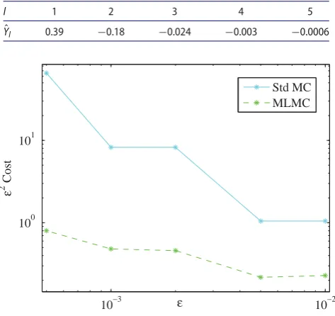
whereB(t)is a scalar Brownian motion. This is a specified Lewis stochastic volatility model. Accord-ing to Examples 3.5 and 3.9 in [22], we sample over 1000 discretized Brownian paths and use stepsizes sl=T/2lforl=1, 2,. . ., 5 in the truncated EM method. LetYˆldenote the sample value ofYl. Here
we setT=1 andh(sl)=s−l 1/4.
Firstly, we show some computational results of the classic EM method with the MLMC method. It can be seen from Table1that the simulation result of (14) computed by the MLMC approach together with the classic EM method is divergent.
The simulation results using the MLMC method combined with the truncated EM method is presented in Table2. It is clear that some convergent trend is displayed.
Table 1.Numerical results using the MLMC with the classic EM method.
l 1 2 3 4 5 ˆ
[image:7.493.129.366.122.345.2]Yl 1.00 2.59e+102 −2.94e+159 – –
Table 2.Numerical results using the MLMC with the truncated EM method.
l 1 2 3 4 5 ˆ
Yl 0.39 −0.18 −0.024 −0.003 −0.0006
10−3 10−2
100 101
ε
2 Cost
ε
Std MC MLMC
Figure 1.Computational cost.
Acknowledgements
The authors would like to thank the referee and editor for their very useful comments and suggestions, which have helped to improve this paper a lot.
Disclosure statement
No potential conflict of interest was reported by the authors.
Funding
The authors would also like to thank the Natural Science Foundation of Shanghai [14ZR1431300], the Royal Soci-ety [Wolfson Research Merit Award WM160014], the Leverhulme Trust [RF-2015-385], the Royal SociSoci-ety of London [IE131408], the EPSRC [EP/E009409/1], the Royal Society of Edinburgh [RKES115071], the London Mathematical Society [11219], the Edinburgh Mathematical Society [RKES130172], the Ministry of Education (MOE) of China [MS2014DHDX020], Shanghai Pujiang Program [16PJ1408000], the Natural Science Fund of Shanghai Normal University [SK201603], Young Scholar Training Program of Shanghai’s Universities for their financial support.
ORCID
X. Mao http://orcid.org/0000-0002-6768-9864
References
[1] Y. Ait-Sahalia,Testing continuous-time models of the spot interest rate, Rev. Financ. Stud. 9 (1996), pp. 385–426. [2] E. Allen,Modeling with Itô Stochastic Differential Equations, Mathematical Modelling: Theory and Applications
[3] D.F. Anderson, D.J. Higham, and Y. Sun,Multilevel Monte Carlo for stochastic differential equations with small noise, SIAM J. Numer. Anal. 54 (2016), pp. 505–529.
[4] S. Dereich and S. Li,Multilevel Monte Carlo for Lévy-driven SDEs: Central limit theorems for adaptive Euler schemes, Ann. Appl. Probab. 26 (2016), pp. 136–185.
[5] S. Dereich and S. Li,Multilevel Monte Carlo implementation for SDEs driven by truncated stable processes, inMonte Carlo and Quasi-Monte Carlo Methods, R. Cools and D. Nuyens, eds., Springer, 2016, pp. 3–27.
[6] C.W. Gardiner,Handbook of Stochastic Methods for Physics, Chemistry and the Natural Sciences, 3rd ed., Springer Series in Synergetics 13, Springer-Verlag, Berlin,2004.
[7] M.B. Giles,Improved multilevel monte carlo convergence using the Milstein scheme, inMonte Carlo and Quasi-Monte Carlo Methods 2006, A. Keller, S. Heinrich, and H. Niederreiter eds., Springer, Berlin, Heidelberg, 2008, pp. 343–358.
[8] M.B. Giles,Multilevel monte carlo path simulation, Oper. Res. 56 (2008), pp. 607–617. [9] M.B. Giles,Multilevel Monte Carlo methods, Acta Numer. 24 (2015), pp. 259–328.
[10] A. Gray, D. Greenhalgh, L. Hu, X. Mao, and J. Pan,A stochastic differential equation SIS epidemic model, SIAM J. Appl. Math. 71 (2011), pp. 876–902.
[11] Q. Guo, W. Liu, X. Mao, and R. Yue,The partially truncated Euler–Maruyama method and its stability and boundedness, Appl. Numer. Math. 115 (2017), pp. 235–251.
[12] N. Halidias,Constructing positivity preserving numerical schemes for the two-factor CIR model, Monte Carlo Methods Appl. 21 (2015), pp. 313–323.
[13] D.J. Higham, X. Mao, and A.M. Stuart,Strong convergence of Euler-type methods for nonlinear stochastic differential equations, SIAM J. Numer. Anal. 40 (2002), pp. 1041–1063.
[14] Y. Hu,Semi-implicit Euler-Maruyama scheme for stiff stochastic equations, inStochastic Analysis and Related Topics, V (Silivri, 1994), H. Körezlioğlu, B. Øksendal, and A.S. Üstünel, eds., Progr. Probab., Vol. 38, Birkhäuser Boston, Boston, MA, 1996, pp. 183–202.
[15] M. Hutzenthaler and A. Jentzen,Numerical approximations of stochastic differential equations with non-globally Lipschitz continuous coefficients, Mem. Amer. Math. Soc. 236 (2015), pp. v+99.
[16] M. Hutzenthaler, A. Jentzen, and P.E. Kloeden,Strong convergence of an explicit numerical method for SDEs with nonglobally Lipschitz continuous coefficients, Ann. Appl. Probab. 22 (2012), pp. 1611–1641.
[17] M. Hutzenthaler, A. Jentzen, and P.E. Kloeden,Divergence of the multilevel Monte Carlo Euler method for nonlinear stochastic differential equations, Ann. Appl. Probab. 23 (2013), pp. 1913–1966.
[18] P. E. Kloeden and E. Platen,Numerical Solution of Stochastic Differential Equations, Applications of Mathematics (New York) Vol. 23, Springer-Verlag, Berlin,1992.
[19] W. Liu and X. Mao,Strong convergence of the stopped Euler–Maruyama method for nonlinear stochastic differential equations, Appl. Math. Comput. 223 (2013), pp. 389–400.
[20] X. Mao,Stochastic Differential Equations and Applications, 2nd ed., Horwood Publishing Limited, Chichester,
2008.
[21] X. Mao,The truncated Euler–Maruyama method for stochastic differential equations, J. Comput. Appl. Math. 290 (2015), pp. 370–384.
[22] X. Mao,Convergence rates of the truncated Euler–Maruyama method for stochastic differential equations, J. Comput. Appl. Math. 296 (2016), pp. 362–375.
[23] G.N. Milstein and M.V. Tretyakov,Stochastic Numerics for Mathematical Physics, Springer-Verlag, Berlin,2004. [24] Y. Niu, K. Burrage, and L. Chen,Modelling biochemical reaction systems by stochastic differential equations with
reflection, J. Theoret. Biol. 396 (2016), pp. 90–104.
[25] B. Øksendal,Stochastic Differential Equations, 6th ed., Universitext Springer-Verlag, Berlin,2003, an introduction with applications.
[26] E. Platen and D. Heath,A Benchmark Approach to Quantitative Finance, Springer Finance, Springer-Verlag, Berlin,
2006.
[27] S. Sabanis,A note on tamed Euler approximations, Electron. Comm. Probab. 18 (2013), pp. 47, 10.
[28] L. Szpruch, X. Mao, D.J. Higham, and J. Pan,Numerical simulation of a strongly nonlinear Ait-Sahalia-type interest rate model, BIT 51 (2011), pp. 405–425.
[29] M.V. Tretyakov and Z. Zhang,A fundamental mean-square convergence theorem for SDEs with locally Lipschitz coefficients and its applications, SIAM J. Numer. Anal. 51 (2013), pp. 3135–3162.
[30] X. Wang and S. Gan,The tamed Milstein method for commutative stochastic differential equations with non-globally Lipschitz continuous coefficients, J. Difference Equ. Appl. 19 (2013), pp. 466–490.
Appendix
Proof of Theorem3.1: Using the notationxto denote the unique integernsatisfying the inequalitiesx≤n<x+1, we start by choosingLto be
L=
log(√2c1Tαε−1) αlogM
, so that 1 √ 2M −αε <c
1sαL ≤ 1 √
2ε. Hence, by the condition 1 and 2 we have
(E[Y]−E[f(X(T))])2
=
E
L
l=0 Yl
−E[f(X(T))]
2
=(E[f(X¯sL(T))−f(X(T))])2
≤(c1sαL)2 1 2ε
2. (A1)
Therefore, we have
(E[Y]−E[f(X)])2≤1 2ε
2.
This upper bound on the square of bias error together with the upper bound of12ε2on the variance of the estimator, which will be proved later, gives a upper bound ofε2to the MSE.
Noting
L
l=0
s−l 1=s−L1
L
i=0
M−i< M M−1s
−1
L ,
using the standard result for a geometric series and the inequality(1/√2)M−αε <c1sαL, we can obtain
s−L1<M
ε
√ 2c1
−1/α
.
Then, we have
L
l=0
s−l1< M M−1s
−1
L <
M2 M−1(
√
2c1)1/αε−1/α. (A2)
We now consider the different possible values ofβand to compare them to theα. (a) Ifβ=1, we setNl= 2ε−2(L+1)c2slso that
V[Y]= L
l=0 V[Yl]≤
L
l=0
c2Nl−1sl≤1 2ε
2,
which is the required.
For the bound of the computational complexityC, we have
C=
L
l=0 Cl≤c3
L
l=0 Nls−l1
≤c3
L
l=0
(2ε−2(L+1)c
2sl+1)s−l 1
≤c3
2ε−2(L+1)2c2+
L
l=0 s−l1
≤c3
2ε−2(L+1)2c2+ M 2
M−1( √
2c1)1/αε−1/α
According to the definition ofL, we have
L≤ logε
−1 αlogM+
log(√2c1Tα) αlogM +1.
Given that 1<logε−1forε <e−1, we have
L+1≤c5logε−1,
where
c5=α 1
logM+max
0,log( √
2c1Tα) αlogM
+2.
Hence, the computation complexity is bounded by
C≤c3(2ε−2c52(logε−1)2c2+ M 2
M−1( √
2c1)1/αε−1/α)
=c3(2ε−2c25(logε)2c2+ M 2
M−1( √
2c1)1/αε−1/α).
So ifα≤(−logε)/log[(logε/ε)2], we have
C≤c3
2c25c2+ M 2
M−1( √
2c1)1/α
ε−1/α.
Ifα > (−logε)/log[(logε/ε)2], we have
C≤c3
2c25c2+ M 2
M−1( √
2c1)1/α
ε−2(logε)2.
(b) Forβ >1, setting
Nl= 2ε−2c2T(β−1)/2(1−M−(β−1)/2)−1s(βl +1)/2,
then we have
V[Y]= L
l=0 V[Yl]≤
L
l=0 c2Nl−1sβl
≤1 2ε
2T−(β−1)/2(1−M−(β−1)/2)L
l=0 s(βl −1)/2.
Using the stand result for a geometric series
L
l=0
s(βl −1)/2=T(β−1)/2
L
l=0
(M−(β−1)/2)l
we obtain that the upper bound of variance is12ε2. So the computation complexity is bounded by
C≤c3
L
l=0 Nls−l1
≤c3
L
l=0
(2ε−2c2T(β−1)/2(1−M−(β−1)/2)−1s(βl +1)/2+1)s−l1
=c3
2ε−2c2T(β−1)/2(1−M−(β−1)/2)−1
L
l=0
s(βl −1)/2+
L
l=0 s−l1
≤c3[2ε−2c2T(β−1)/2(1−M−(β−1)/2)−1T(β−1)/2(1−M−(β−1)/2)−1
+ M2 M−1(
√
2c1)1/αε−1/α]
=c3
2ε−2c2Tβ−1(1−M−(β−1)/2)−2+ M 2
M−1( √
2c1)1/αε−1/α
.
So whenα≥12, we have
C≤c3[2c2Tβ−1(1−M−(β−1)/2)−2+ M 2
M−1( √
2c1)1/α]ε−2,
Whenα < 1 2, we have
C≤c3
2c2Tβ−1(1−M−(β−1)/2)−2+ M 2
M−1( √
2c1)1/α
ε−1/α.
(c) For 0< β <1, setting
Nl= 2ε−2c2s−L(1−β)/2(1−M−(1−β)/2)−1s(βl +1)/2, then we have
V[Y]= L
l=0 V[Yl]≤
L
l=0 c2Nl−1sβl
≤1 2ε
2s(1−β)/2
L (1−M−(1−β)/2) L
l=0
s−l(1−β)/2.
Because
L
l=0
s−l (1−β)/2=s−L(1−β)/2
L
l=0
(M−(1−β)/2)l
<s−L(1−β)/2(1−M−(1−β)/2)−1, (A4)
we obtain the upper bound on the variance of the estimator to be12ε2. Finally, using the upper bound ofNl, the computational complexity is
C≤c3
L
l=0 Nls−l1
≤c3
L
l=0
(2ε−2c2sL−(1−β)/2(1−M−(1−β)/2)−1sl(β+1)/2+1)s−l 1
=c3[2ε−2c2sL−(1−β)/2(1−M−(1−β)/2)−1 L
l=0
s−l(1−β)/2+
L
l=0 s−l 1]
≤c3[2ε−2c2sL−(1−β)(1−M−(1−β)/2)−2+ L
where (A4) is used in the last inequality.
Moreover, because of the inequality(1/√2)M−αε <c1sαL, we have
s−L(1−β)< (√2c1)(1−β)/αM1−βε−(1−β)/α,
then
C≤c3[2ε−2c2sL−(1−β)(1−M−(1−β)/2)−2+ L
l=0 s−l 1]
≤c3[2ε−2c2( √
2c1)(1−β)/αM1−βε−(1−β)/α(1−M−(1−β)/2)−2+
L
l=0 s−l1]
≤c3[2ε−2c2( √
2c1)(1−β)/αM1−βε−(1−β)/α(1−M−(1−β)/2)−2+ M 2
M−1( √
2c1)1/αε−1/α]
=c3[2c2( √
2c1)(1−β)/αM1−β(1−M−(1−β)/2)−2ε−2−(1−β)/α+ M 2
M−1( √
2c1)1/αε−1/α].
Ifβ≤2α, thenε−2−(1−β)/α> ε−1/α, so we have
C≤c3[2c2( √
2c1)(1−β)/αM1−β(1−M−(1−β)/2)−2+ M 2
M−1( √
2c1)1/α]ε−2−(1−β)/α.
Ifβ >2α, thenε−2−(1−β)/α< ε−1/α, so we have
C≤c3
2c2( √
2c1)(1−β)/αM1−β(1−M−(1−β)/2)−2+ M 2
M−1( √
2c1)1/α