City, University of London Institutional Repository
Citation
:
Soch, J., Haynes, J-D. and Allefeld, C. ORCID: 0000-0002-1037-2735 (2016). How to avoid mismodelling in GLM-based fMRI data analysis: cross-validated Bayesian model selection. NeuroImage, 141, pp. 469-489. doi: 10.1016/j.neuroimage.2016.07.047This is the accepted version of the paper.
This version of the publication may differ from the final published
version.
Permanent repository link:
http://openaccess.city.ac.uk/id/eprint/22847/Link to published version
:
http://dx.doi.org/10.1016/j.neuroimage.2016.07.047Copyright and reuse:
City Research Online aims to make research
outputs of City, University of London available to a wider audience.
Copyright and Moral Rights remain with the author(s) and/or copyright
holders. URLs from City Research Online may be freely distributed and
linked to.
City Research Online: http://openaccess.city.ac.uk/ [email protected]
How to avoid mismodelling
in GLM-based fMRI data analysis:
cross-validated Bayesian model selection
—
Preprint, resubmitted to
NeuroImage
on 31/05/2016
—
Joram Soch
a,f,•, John-Dylan Haynes
a,b,c,d,e,f, Carsten Allefeld
a,ba Bernstein Center for Computational Neuroscience, Berlin, Germany
b Berlin Center for Advanced Neuroimaging, Berlin, Germany
c Berlin School of Mind and Brain, Berlin, Germany
d Excellence Cluster NeuroCure, Charit´e-Universit¨atsmedizin Berlin, Germany
e Department of Neurology, Charit´e-Universit¨atsmedizin Berlin, Germany
f Department of Psychology, Humboldt-Universit¨at zu Berlin, Germany
• Corresponding author: [email protected].
BCCN Berlin, Philippstraße 13, Haus 6, 10115 Berlin, Germany.
Abstract
Voxel-wise general linear models (GLMs) are a standard approach for analyzing func-tional magnetic resonance imaging (fMRI) data. An advantage of GLMs is that they are flexible and can be adapted to the requirements of many different data sets. How-ever, the specification of first-level GLMs leaves the researcher with many degrees of freedom which is problematic given recent efforts to ensure robust and reproducible fMRI data analysis. Formal model comparisons that allow a systematic assessment of GLMs are only rarely performed. On the one hand, too simple models may underfit data and leave real effects undiscovered. On the other hand, too complex models might overfit data and also reduce statistical power. Here we present a systematic approach termed cross-validated Bayesian model selection (cvBMS) that allows to decide which GLM best describes a given fMRI data set. Importantly, our approach allows for non-nested model comparison, i.e. comparing more than two models that do not just differ by adding one or more regressors. It also allows for spatially heterogeneous modelling, i.e. using different models for different parts of the brain. We validate our method using simulated data and demonstrate potential applications to empirical data. The increased use of model comparison and model selection should increase the reliability of GLM results and reproducibility of fMRI studies.
Keywords
1
Introduction
Over the last 20 years, thegeneral linear model (GLM; Friston et al., 1994; Holmes and
Friston, 1998) has been the main workhorse in the analysis of functional neuroimaging data. Though many alternatives are available – e.g. network modelling approaches (Smith et al., 2011) such as dynamic causal modelling (Friston et al., 2003), multivariate pat-tern analysis (Haxby, 2012) or representational similarity analysis (Kriegeskorte et al., 2008) –, the GLM approach remains the most important analysis method for task-based
experiments using functional magnetic resonance imaging (fMRI), among other reasons
because it is well understood and highly flexible.
However, this flexibility has its drawbacks as well. Using the GLM, a researcher has to make a lot of modelling decisions – which processes to consider relevant, which experi-mental events to model and in which detail, which hemodynamic basis set to use etc. –, many of which strongly influence the sensitivity of the analysis. This situation tempts the
researcher to run not just one analysis based ona priori information about the paradigm
and previous experience or general recommendations (Josephs and Henson, 1999; Grin-band et al., 2008), but to try many different models until good results are obtained (Leek
and Peng, 2015). This strategy, a form of so-called p-hacking (Simonsohn et al., 2014),
may render the false positive rate much higher than indicated by the nominal significance
level (Simmons et al., 2011) and is one of the reasons for recent doubt about the
repro-ducibility of neuroimaging studies (Pernet and Poline, 2015; Glatard et al., 2015). On the other hand, the obvious solution – to decide for a single analysis pipeline in advance and
refrain from post-hoc modifications, a procedure referred to as pre-registration (Boekel
et al., 2015) – often leads to a suboptimal model which may fail to detect a real effect. In this paper, we propose a different approach: to select an optimal model from a number of candidate models, but without recourse to the statistical significance of a test based
on this model. Instead, we applyBayesian model selection (BMS; MacKay, 2003; Bishop,
2007) to general linear models. Note that we do not propose to replace null hypothesis tests with Bayesian procedures, but only suggest to select the optimal model via BMS
and then apply a standard GLM-based hypothesis test (t-test or F-test).
In the following section, we examine the problem ofmodel misspecification in more detail,
2
Background
2.1
Model misspecification
For almost every psychological paradigm that can be implemented as an fMRI experiment, there exist several plausible ways to model it in a GLM (Monti, 2011; Carp, 2012). Typical questions that occur in setting up the analysis include: Should one include this regressor of no interest or not? Does this cognitive process represent the baseline or must it be considered activation? What is the duration of the underlying neuronal process? Should one model cue stimuli, button presses, error trials or feedback screens? How should the hemodynamic response be modeled? etc. If decisions are made that do not satisfy the data, this leads to a misspecified model.
Two basic forms of mismodelling areunderfitting and overfitting (Guyon and Yao, 1999;
see also MacKay, 2003; Bishop, 2007). In the first case, a necessary regressor is omitted from the model which reduces the model’s descriptive power with respect to the given data (increasing the in-sample error). For example, the subject’s reaction times (RT) in task-based fMRI experiments can account for a considerable amount of signal variance (Grinband et al., 2011; Yeung et al., 2011) so that omitting an RT regressor from the GLM would cause underfitting. In the second case, unnecessary regressors are included in the model, which are then just fitted to noise and thereby reduce the model’s descriptive power with respect to other data of the same kind (increasing the generalization error). For example, global signal regression (GSR) in resting-state fMRI might induce spurious anti-correlations (Murphy et al., 2009; Chai et al., 2012) so that including it in the model would cause overfitting. It is also possible that a relevant effect is modeled, but the regressor does not have the optimal shape, e.g. because the assumed hemodynamic response function (HRF) does not reflect the actual hemodynamic response (Monti, 2011). Since this can be seen as omitting the correct regressor but including a wrong one, in this case overfitting and underfitting occur at the same time. From the the perspective of a hypothesis test based on the respective model, underfitting increases the residual error while overfitting decreases the error degrees of freedom which is why in consequence both reduce the sensitivity (power) of the test.
These theoretical considerations are supported by empirical evidence of potential under-fitting (Lieberman and Cunningham, 2009), potential overunder-fitting (Eklund et al., 2012) and potential p-hacking (Vul et al., 2009). It has also been demonstrated that activations detected using GLM-based fMRI analysis substantially depend on the model which is employed and its particular assumptions (Carp, 2012). Since these are only rarely scru-tinized during GLM specification, mismodelling can be considered a serious problem in fMRI data analysis (Monti, 2011).
An alternative way to describe under- and overfitting is through the concepts of
2.2
Previous measures against model misspecification
In practice, when faced with the question whether a particular regressor should be in-cluded in a model, sometimes a null hypothesis test is performed to make this decision (see e.g. Henson et al., 2001). A statistical parametric map for the corresponding param-eter is computed at the group level, and the regressor is included if there are significant effects in brain areas that are thought to be relevant for the paradigm. There are several disadvantages to this approach: First, it is restricted to nested model comparison (Penny, 2012), i.e. choosing between two models that only differ by including or not including a regressor (or a set of regressors). Second, it only measures the gain in model accuracy through better fit (lower residual variance), but not model complexity and how well it generalizes to other data (Oaksford, 2002) which is only indirectly accounted for via e.g. numerator degrees of freedom in the F-statistic. Third, it also fails to detect the relevance of regressors that have a non-significant effect at the group level, but still contribute to model fit on the level of individual subjects (Rigoux et al., 2014).
Beyond this na¨ıve approach, the problem of model misspecification in fMRI analysis has been recognized by researchers and a number of strategies have been developed to deal with potential mismodelling. Kherif and Loh have proposed algorithms for model opti-mization, but they only allow inference pertaining to nested model comparisons (Kherif et al., 2002) and condition regressor timing (Loh et al., 2008). Razavi et al., 2003 investi-gated model accuracy based on the goodness of fit, but do not consider model complexity. Luo and Nichols, 2003 have supplied a range of frequentist methods for the diagnosis of a given model and exploratory data analysis. Measures against overfitting were proposed for certain situations, e.g. noise-model selection (Penny et al., 2007b) and hemodynamic response modelling (Kay et al. 2008a). In addition, there are some recommendations regarding the temporal specification of experimental conditions (Josephs and Henson, 1999; Yarkoni et al., 2009), orthogonalisation of regressors (Mumford et al., 2015) and modelling of non-white noise (Lund et al., 2006). However, none of these methods and rec-ommendations provide a general remedy for all possible forms of model misspecification and they are not based on systematic model comparison.
2.3
General linear model selection for fMRI data analysis
An approach that avoids these shortcomings is Bayesian model selection (BMS). One
reason for this is that it uses the Bayesian log model evidence (LME) as a measure of
model quality, a measure which accounts for both model accuracy and model complexity, so that maximizing it avoids both underfitting and overfitting (MacKay, 2003; Bishop,
2007). Moreover, it attaches a model quality to any GLM and therefore enables
non-nested model comparison, i.e. comparing more than two models that do not just differ by one or more regressors but in arbitrary ways (Penny, 2012).
The concept of Bayesian model selection is not new to neuroimaging. In dynamic causal modelling (DCM; Friston et al., 2003; Stephan et al., 2008), the free energy, a variational approximation to the log model evidence (Friston et al., 2007) is an established measure
to quantify model quality (Penny et al., 2004). For the GLM, the past has seenVariational
we introduce a number of methodological improvements which address shortcomings of these approaches and increase the usability of BMS across GLMs for fMRI.
First, a practical problem for the use of BMS is that it requires prior distributions on the model parameters. Using too wide priors will exaggerate the complexity of models which include more regressors while too narrow priors will underestimate it. Optimally, pri-ors should be informed by previous experience about typical parameter values (Stephan, 2010). However, such numeric information is normally not included in neuroimaging pa-pers and concrete values strongly depend, among others, on scanner technology (Tri-antafyllou et al., 2005). We here solve this problem by using part of the available data to obtain an informative prior and another part to calculate the log model evidence,
leading to the cross-validated log model evidence (cvLME). BMS based on this quantity
is referred to as cross-validated Bayesian model selection (cvBMS).
Second, as opposed to previous Bayesian analyses (Penny et al., 2003, 2005, 2007a), we use a simple, but reasonable model structure which exactly corresponds to the model un-derlying standard first-level fMRI data analyses (Friston et al., 1994) as performed e.g. by
Statistical Parametric Mapping (SPM). This enables anAnalytical Bayesian computation
for the Bayesian GLM with normal-gamma priors (GLM-NG) which makes our method both fast and precise.
The cvLME for the GLM-NG is combined with a voxel-wise implementation of
random-effects Bayesian model selection (RFX BMS; Stephan et al., 2009; Rosa et al., 2010; Penny et al., 2010; Rigoux et al., 2014), a common procedure for second-level model inference that accounts for the optimal model to vary across voxels as well as subjects.
This allows for spatially heterogeneous modelling, i.e. using different models for different
areas of the brain (Razavi et al., 2003).
2.4
Application of the method
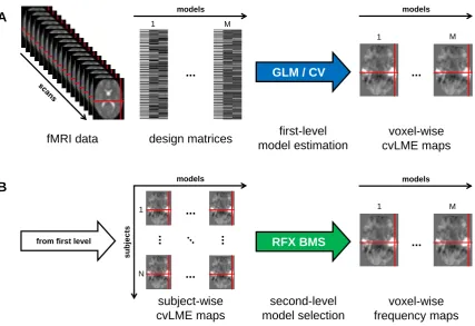
On the first level, once a model is specified and estimated for a given subject, cvBMS calculates a cross-validated version of the log model evidence (cvLME) for each voxel in the brain. This results in a cvLME map which quantifies the model’s performance in different parts of the brain (see Figure 1A). The cvLME is a relative measure of model quality and its absolute value has no direct interpretation.
For a single subject, two or more models are compared by converting the log model
evidences jointly into posterior model probabilities. If the models fall into one or more
model families, where models of a family have a particular modelling decision in common, log model evidences can be first aggregated into log family evidences which are then
converted into posterior family probabilities. The optimal model or model family is the
one with the largest posterior probability.
On the second level, cvBMS accounts for the fact that different models may be optimal in different subjects. Using the first-level log model (or family) evidences for all models (or families) in all subjects, it estimates how frequently each model is optimal in the
population of subjects. The results are brain maps of estimated model frequencies (see
Figure 1B) or, alternatively, maps of the posterior probability that a given model is more
frequent than all others, the so-calledexceedance probability. The optimal model or model
family is the one with the largest estimated frequency.
and have the form of brain maps. Selecting models on a voxel-by-voxel basis results in a selected-model map (SMM) which can then be used to restrict GLM-based analyses to those voxels where the corresponding model is optimal.
A
B
fMRI data
models
design matrices
models
voxel-wise cvLME maps
...
... GLM / CV
first-level model estimation
models models
subject-wise cvLME maps
voxel-wise frequency maps second-level
model selection
su
b
ject
s
...
... ...
...
1
N
1 M
RFX BMS
from first level ...
1 M
[image:7.595.83.511.150.443.2]1 M
Figure 1. Model selection for general linear models in fMRI data analysis. This figure summarizes our approach of cross-validated Bayesian model selection (cvBMS). All calcu-lations are performed voxel-wise, an exemplary voxel is highlighted using red crosshairs. (A) First level: All fMRI data from one subject and design matrices for each model enter general linear model estimation (GLM) with cross-validation across sessions (CV) which produces voxel-wise cross-validated log model evidence (cvLME) maps for each model on which population inference is based. (B) Second level: The cvLME images from all
subjects (N = number of subjects) and all models (M = number of models) enter
3
Theory
In this section, we describe in detail the mathematical derivation of our proposed method. For the non-technical reader mainly interested in the practical use of the method, we recommend to directly proceed to Section 4 demonstrating the application of the method to empirical data.
3.1
The general linear model
As linear models, GLMs for fMRI (Friston et al., 1994; Kiebel and Holmes, 2011) assume an additive relationship between experimental conditions and the fMRI BOLD signal, i.e. a linear summation of expected hemodynamic responses into the measured hemodynamic
signal. Consequently, in the GLM, a single voxel’s fMRI data (y) are modelled as a linear
combination (β) of experimental factors and potential confounds (X), where errors (ε)
are assumed to be normally distributed around zero and to have a known covariance
structure (V), but unknown variance factor (σ2):
y=Xβ+ε, ε∼N(0, σ2V) (1)
In this equation, X is an n×p matrix called the “design matrix” and V is an n×n
matrix called a “correlation matrix” where n is the number of data points and p ist the
number of regressors. In standard analysis packages like Statistical Parametric Mapping
(SPM) (Ashburner et al., 2013),V is typically estimated from the signal’s temporal
auto-correlations across all voxels using a Restricted Maximum Likelihood (ReML) approach
(Friston et al., 2002b, a). In contrast to that, X has to be constructed by the user which
is essential to the specification of a GLM (Monti, 2011). As there are often many possible models for a given psychological paradigm, GLMs for fMRI need to be subjected to model selection in order to avoid model misspecification.
The general linear model in (1) implicitly defines the following likelihood function:
p(y|β, σ2) = N(y;Xβ, σ2V) (2)
Classical estimation of the GLM proceeds by maximizing the likelihood functionp(y|β, σ2)
with respect to the unknown parameterβto find the optimal parameter estimates. Under
temporal independence, i.e. ifV =In, this Maximum Likelihood (ML) solution is obtained
by Ordinary Least Squares (OLS) estimation (Bishop, 2007, eq. 3.15).
IfV is not equal to the identity matrix In, i.e. errorsε are not assumed independent and
identically distributed (i.i.d.), Weighted Least Squares (WLS) estimation is employed which gives rise to Gauss-Markov (GM) estimates (Koch, 2007, eq. 4.29). This WLS
solution is equivalent to multiplying data y and design X with a whitening matrixW =
V−1/2 and then performing OLS estimation.
Statistical inference proceeds by multiplying the parameter estimates ˆβ with a contrast
vector or matrixcand thresholding statistical parametric maps (SPM) to perform a t-test
or an F-test on the parameter estimates (Stephan, 2010).
3.2
Bayesian inference for the GLM
Classical and Bayesian estimation agree in their use of the likelihood given by equation
(2). For mathematical convenience, we rewrite the likelihood function in terms of ann×n
precision matrix P =V−1 and the inverse residual varianceτ = 1/σ2:
p(y|β, τ) = N(y;Xβ,(τ P)−1) (3)
Other than classical inference, Bayesian inference requires prior distributions on the model parameters. The straightforward choice of prior distribution for the general linear model
with unknown regression coeffcients β and inverse residual variance τ is the conjugate
prior relative to this likelihood function (Koch, 2007, ch. 4.3.2; Bishop, 2007, ch. 3.3), the normal-gamma distribution (Koch, 2007, eq. 2.212; Bishop, 2007, eq. B.52)
p(β|τ) = N(β;µ0,(τΛ0)−1)
p(τ) = Gam(τ;a0, b0)
(4)
where µ0 and Λ0 are the prior mean and the prior precision of β and a0 and b0 are the
prior shape and rate parameters for τ (Gelman et al., 2013, p. 68).
Bayes’ theorem implies that the posterior is proportional to the product of likelihood and prior. As we show in Appendix A, the likelihood function from (3) and the parameter prior from (4) result in the following posterior distribution on the model parameters
p(β|τ, y) = N(β;µn,(τΛn)−1)
p(τ|y) = Gam(τ;an, bn)
(5)
where the posterior parameters are given by (Koch, 2007, eq. 4.159)
µn= Λ−n1(X
TP y+ Λ 0µ0)
Λn=XTP X + Λ0
an=a0+
n
2
bn=b0+ 1 2(y
T
P y+µT0Λ0µ0−µTnΛnµn)
(6)
By calculating a posterior distribution, we update our belief about the model parameters regarding their location and precision. Upon model estimation, this posterior distribution
can be used for statistical inference about the unknown parameters β and τ.
3.3
The Bayesian model evidence
Consider Bayesian inference on data y using model m with parameters θ. In this case,
Bayes’ theorem is a statement about the posterior density (Gelman et al., 2013, eq. 1.1):
The denominatorp(y|m) acts as a normalization constant on the posterior densityp(θ|y, m) and is given by (Gelman et al., 2013, eq. 1.3)
p(y|m) = Z
p(y|θ, m)p(θ|m) dθ (8)
This is the probability of the data given only the model, independent of any particular parameter values. It is also called “marginal likelihood” or “model evidence” and can act as a model quality criterion in Bayesian inference, because parameters are integrated out of the likelihood (Penny, 2012). For computational reasons, only the logarithmized or log
model evidence (LME) L(m) = logp(y|m) is of interest in most cases.
As we show in Appendix B, the log model evidence for the GLM-NG is given by
L(m) = 1
2log|P| −
n
2 log(2π) + 1
2log|Λ0| − 1
2log|Λn|+ log Γ(an)−log Γ(a0) +a0logb0−anlogbn
(9)
where the posterior parameters are given by equation (6).
3.4
Accuracy and Complexity
Recall Bayes’ theorem for model-based inference on unknown parameters θ given by
equation (7). Rearranging this equation, the model evidence can also be written as
p(y|m) = p(y|θ, m)p(θ|m)
p(θ|y, m) (10) Logarithmizing both sides of the equation and taking the expectation with respect to the
posterior density over model parameters θ gives (Penny et al., 2007a, eq. 8)
L(m) =
Z
p(θ|y, m) logp(y|θ, m) dθ−
Z
p(θ|y, m) logp(θ|y, m)
p(θ|m) dθ (11) Using this reformulation, the LME as a model quality measure can be naturally decom-posed into an accuracy term, the posterior expected log likelihood, and a complexity penalty, the Kullback-Leibler (KL) divergence (Kullback and Leibler, 1951) between the posterior and the prior distribution (Friston et al., 2007; Penny et al., 2007a)
L(m) = Acc(m)−Com(m)
Acc(m) =hlogp(y|θ, m)ip(θ|y,m) Com(m) = KL [p(θ|y, m)||p(θ|m)]
(12)
The log model evidence is superior to other model quality criteria like Akaike’s informa-tion criterion (AIC) (Akaike, 1974) or Bayesian informainforma-tion criterion (BIC) (Schwarz, 1978) in two ways. First, in the accuracy term, it does not use frequentist point estimates
like the ML, but accounts for the possible uncertainty about model parameters θ.
Sec-ond, in the complexity penalty, different parameters receive different complexities which accounts for the fact that model parameters might be correlated (Penny, 2012) or might introduce a different degree of flexibility into the model.
3.5
Cross-validated log model evidence
These benefits of the Bayesian model evidence come at the cost of having to specify prior distributions on the model parameters (Gelman, 2008). However, in fMRI data analysis with new or modified experimental paradigms and different types of scanners or scanning protocols, such prior information is usually not at hand. Non-informative priors can be used in this absence of knowledge, but they are usually improper and let the model evidence diverge. However, improper priors can lead to proper posteriors. We therefore use a non-informative prior for estimating the model from the data of all but one session and then employ the resulting posterior distribution as an informative prior, allowing us to compute the model evidence for the left-out session.
In more detail, we perform S-fold cross-validation where S is the number of sessions,
and priors in each session are calculated as posteriors from all other sessions.1 Using
non-informative (improper) priors for the combined data y¯s from S−1 sessions ¯s (e.g.
¯
s = {1,2,3,4}), we obtain combined posteriors p(θ|y¯s). Using these posteriors as
infor-mative (proper) priors in the remaining session s (i.e. s = 5) and based on the common
assumption of statistical independence between sessions, we obtain an out-of-sample log model evidence (oosLME) as follows:
logp(ys|m) = log Z
p(ys|θ, m)p(θ|ys¯, m) dθ (13)
This procedure embodies the Bayesian maxim that “today’s posterior can be tomorrow’s prior” (Stephan, 2010) and is similar to the log predictive density score (LPDS) approach (Villani et al., 2009; Li et al., 2010). The cross-validated log model evidence (cvLME) is then given by
logp(y|m) = S X
i=1
logp(yi|m) (14)
As non-informative priors for cross-validation in the context of GLMs for fMRI, we use a normal-gamma distribution given in equation (4) with the prior parameters
µ0 = 0p, Λ0 = 0pp and a0 = 0, b0 = 0 (15) which yields an infinitely wide and therefore flat Gaussian for the regression coefficients
β (Friston et al., 2002b) and Jeffreys prior for the inverse residual variance τ (Jeffreys,
1946). As one can see from equation (6), these (improper) priors are non-informative in the sense that only the data remain to influence the (proper) posteriors.
3.6
First-level Bayesian model inference
If several models m of the same datay can be specified, the model evidence can be used
for model inference. In the simplest case of only two models, Bayes factors (BF) or log Bayes factors (LBF) are used for model comparison (Koch, 2007, eq. 3.67):
LBFi,j = logp(y|mi)−logp(y|mj) (16)
Evidence in favor of one model is usually considered “strong” when the LBF exceeds
three, meaning that seeing the data y is about exp(3) ≈ 20 times more likely under
modelmi thanmj (Kass and Raftery, 1995). In the case of two or more models, posterior
model probabilities can be calculated using Bayes’ theorem (Penny et al., 2010):
p(m|y) = p(y|m)p(m) PM
i=1p(y|mi)p(mi)
(17)
One can also consider a model family f, i.e. a set of models m that share some
charac-teristic (Stephan et al., 2009), e.g. certain parameters like a set of regressors in the case of the GLM. Using the law of marginal probability, a family evidence can be calculated from the evidences of the models belonging to this family as follows:
p(y|f) = X m∈f
p(y|m)p(m|f) (18)
If models or families are to be compared in several subjects, it is advisable to use an explicit population proportion model which will be described in the next section.
3.7
Second-level Bayesian model selection
On the second level, between-subject variance in individual model preferences can be
accounted for by a hierarchical model in which first-level model evidencesp(yi|mj) (model
j applied to subject i) serve as the second-level likelihood function p(y|m). Models m
are then assumed to follow a multinomial distribution with model frequencies r and a
Dirichlet distribution with concentration parameters α is used as the prior distribution
for model frequencies r.
This extension of P´olya’s urn model (Mahmoud, 2008), also called random-effects Bayesian
model selection (RFX BMS), has been introduced and validated (Stephan et al., 2009), extended and refined (Penny et al., 2010) and revisited (Rigoux et al., 2014). It is widely applied (Stephan et al., 2010) in dynamic causal modelling (DCM) and was also imple-mented for voxel-wise model inferences (Rosa et al., 2010).
An iterative estimation algorithm has been developed to infer a posterior distribution
over model frequencies p(r|y) from prior concentration parameters α0 (Stephan et al.,
2009). This procedure and the model are given in detail in Appendix D. In this work, we
apply RFX BMS to cvLMEs from the first level and use a uniform prior over r. Then,
the posterior distribution overr informs us about the proportion of the population whose
3.8
Decision-theoretic model choice
In DCM, it is common practice (see e.g. Deserno et al., 2012) to report group-level model selection results using exceedance probabilities (EP), i.e. the posterior probability of a model being more frequent than any other model (Stephan et al., 2009; Penny et al., 2010). Additionally, RFX BMS also gives rise to estimated model frequencies in the form
of expected frequencies (EF), i.e. the posterior means hri, or likeliest frequencies (LF),
i.e. the posterior modes ˆrMAP. When a uniform prior is used, LFs directly quantify the
proportion of subjects in the sample in which a particular model is optimal.
In model selection, we are not so much interested in inference about the model frequencies
r, but rather in an optimal decision regarding the models m, i.e. which model to use to
analyze a group of subjects. As we show in Appendix E, this optimal model choice can be finessed using Bayesian decision theory (BDT) and is achieved by choosing the model with the largest estimated frequency (EF or LF) in an RFX BMS.
4
Validation: empirical data
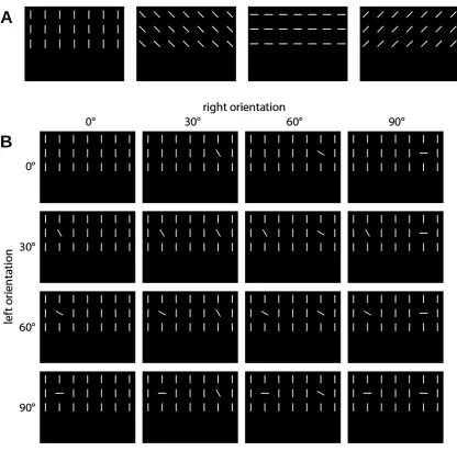
We demonstrate and validate the cvBMS approach using empirical fMRI data acquired in a sample of 22 subjects using orientation pop-out processing (Bogler et al., 2013).
In this experiment, the screen showed a 3×7 array of homogeneous bars oriented either 0°,
45°, 90°or 135°relative to the vertical axis (see Figure 2A). This background stimulation
changed every second and during each trial, one target bar on the left and one target bar
on the right were independently rotated either 0°, 30°, 60° or 90° relative to the rest of
the stimulus display (see Figure 2B). Those trials of orientation contrast (OC) lasted 4 seconds and were alternated with inter-trial intervals of 7, 10 or 13 seconds.
Below the grid of bars in central position, a square was presented that opened up to the left or to the right side for 1 second every 2 seconds. Subjects were asked to indicate via button press whether the square opened up to the same side or the opposite side relative to the last opening.
This study also included a localizer paradigm in which a single bar identical to one of the target bars from the main experiment (see Figure 2B) was presented in blocks. These blocks were separated by intervals of no stimulation.
fMRI data was preprocessed using SPM8, Revision 5236 per 04/02/2013 (http://www.fil. ion.ucl.ac.uk/spm/software/spm8/). Functional MRI scans were corrected for acquisition time delay (slice timing) and head motion (spatial realignment), normalized to MNI space
and smoothed with a Gaussian kernel with an FWHM of 6×6×6 mm.
For the localizer data, a GLM with two regressors, left and right visual stimulation, was estimated. At the group level, two paired t-tests (left vs. right and vice versa) were per-formed to define regions of interest (ROI) that were found to be responsive to oriented bars in the left and right hemisphere (Bogler et al., 2013). Statistical inference was
per-formed using family-wise error (FWE) correction, a significance level of p≤0.05 and an
extent threshold of k = 10. The resulting localizer masks were used to look for model
B
A
Figure 2. Experimental paradigm for orientation pop-out processing. This figure
de-scribes the psychological paradigm used in our empirical validation data set. (A) A 3×7
background display of homogeneously oriented bars rotated by 0°, 45°, 90° or 135° was
alternated every second. (B) During each four-second trial, one bar on the left and one
bar on the right were randomly rotated 0°, 30°, 60° or 90° counter-clockwise relative to
4.1
1st model space: technical model parameters
In the first model space, we begin with the most common approach and build a model with one onset regressor per experimental condition, leading to 16 regressors per session. We include motion parameters from spatial realignment, we activate temporal filtering
using a high-pass filter at T = 128 s and we choose temporal non-sphericity correction
using a first-order auto-regressive AR(1) model. The feature that varies over models is the number of hemodynamic response function (HRF) kernels. In the first model, box-car stimulus functions are convolved with a canonical hemodynamic response function (cHRF) as implemented in SPM. In the second model (cHRF+1), we additionally include the temporal derivative of the cHRF. In the third model (cHRF+2), we include the temporal and dispersion derivative of the cHRF (Henson et al., 2002).
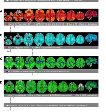
Using group-level model selection and subsequent generation of selected-model maps, we find that the cHRF does not underfit and is sufficient in almost all parts of the brain (see Figure 3A). There are regions in cerebral cortex, potentially belonging to the dorsal attention network (DAN) (Fox et al., 2005, 2006), that require cHRF+1, but no voxels where cHRF+2 was selected. Since the temporal derivative can account for differences in the latency of the peak response (Henson et al., 2001), this could indicate that the HRF peaks earlier or later in DAN regions. As the dispersion derivative can capture differences in the duration of the peak response (Henson et al., 2001), this suggests that the duration of the peak response does not vary significantly across voxels.
4.2
2nd model space: modelling experimental factors
For the second model space, we use the winning model with a canonical HRF and no HRF derivatives as a starting point and focus on different ways of modelling the neural processes underlying the perception of orientation contrast (OC). The model introduced above (GLM I) considers the experiment a factorial design with two factors (left vs.
right OC) having four levels (0°, 30°, 60°, 90°) each. This results in 4×4 = 16 possible
combinations or experimental conditions modelled by 16 onset regressors convolved with the canonical HRF.
The second model (GLM II) puts all trials from all conditions into one HRF-convolved regressor and encodes orientation contrast using a parametric modulator that is given as
PM = deg
90°
with deg = (0°,30°,60°,90°), resulting in PM = (0,1/3,2/3,1), such that the parametric modulator is proportional to orientation contrast. There was one PM for each factor of the design, i.e. one PM for left OC and one PM for right OC.
In behavioral pre-tests for the original study, it was observed that reaction time is not linear in orientation contrast. Instead, the reaction time when being presented with the respective OC and asked to detect where OC occured saturates at lower levels for higher OC (Bogler et al., 2013). Thus, a further model was implemented.
■GLM III [no confounds] ■GLM III-S [plus stimulus] ■GLM III-R [plus response] ■GLM III-S/R [including both] ■GLM II [linear-parametric model] ■GLM III [nonlinear-parametric model]
■GLM I [categorical model] ■GLMs II & III [parametric models]
■GLM cHRF [canonical HRF] ■GLM cHRF+1 [plus one derivative] ■GLM cHRF+2 [plus two derivatives]
A
B
C
D
■initial model choice: 16 regressors, movement parameters, implicit baseline, T = 128 s, AR(1)
[image:17.595.119.476.87.465.2]■final model choice: GLM III, used for further analysis of model preference within V4 (see Figure 5)
whole-brain
V1 V4
left right left right
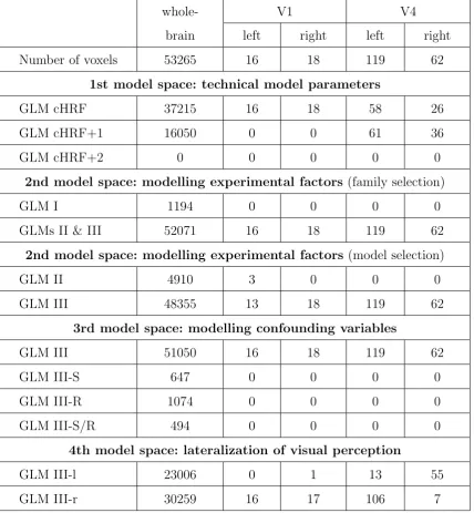
Number of voxels 53265 16 18 119 62
1st model space: technical model parameters
GLM cHRF 37215 16 18 58 26
GLM cHRF+1 16050 0 0 61 36
GLM cHRF+2 0 0 0 0 0
2nd model space: modelling experimental factors (family selection)
GLM I 1194 0 0 0 0
GLMs II & III 52071 16 18 119 62
2nd model space: modelling experimental factors (model selection)
GLM II 4910 3 0 0 0
GLM III 48355 13 18 119 62
3rd model space: modelling confounding variables
GLM III 51050 16 18 119 62
GLM III-S 647 0 0 0 0
GLM III-R 1074 0 0 0 0
GLM III-S/R 494 0 0 0 0
4th model space: lateralization of visual perception
GLM III-l 23006 0 1 13 55
[image:18.595.85.514.73.537.2]GLM III-r 30259 16 17 106 7
PM = deg1 30° + 1
with deg = (0°,30°,60°,90°), resulting in PM = (1,1/2,1/3,1/4), such that the paramet-ric modulator is proportional to the expected average reaction time. This OC model is intended to be a psychologically more plausible description of the neural processing underlying OC perception.
This model space is equivalent to the set of three models already used in the original publication (Bogler et al., 2013). We will refer to GLM I as the “categorical model”, GLM II as the “linear-parametric model” and GLM III as the “nonlinear-parametric model”. In all models, background stimulation was treated as implicit baseline so that only target onsets were explicitly modelled. Note that these models are not nested in each other and therefore significance testing of additional regressors is not applicable for model selection. Furthermore, we cannot just use the best model in each single subject as this would make second-level analysis impossible due to different model parameters.
4.2.1 Accuracy and Complexity
First, just consider GLM I and GLM II. These two models encode exactly the same information, namely the values of the factors “left OC” and “right OC” at each point in time. However, they represent this information in different ways: Whereas the parametric model assumes a parametric shape of the measured signal, the categorical model allows for a greater flexibility of activation patterns across experimental conditions. This means that every signal that can be identified using GLM II can also be detected using GLM I, but not vice versa.
We performed group-level model selection on the cross-validated log model evidences (cvLME) to find voxels where GLM II has a higher model frequency than GLM I. Due to the specific assumptions in GLM II and the higher flexibility of GLM I, we hypothesized that GLM I and GLM II might be equal in terms of model accuracy and the difference would primarily come from on a complexity advantage of GLM II over GLM I. Within left V4, which is known to be sensitive to orientation contrast (Burrows and Moore, 2009; Bogler et al., 2013), we identified the peak voxel (likeliest frequency (LF) = 86.29%,
ex-ceedance probability (EP) = 99.97%, [x y z] = [−18,−76,−8] mm) and extracted cvLME
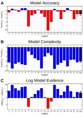
as well as model accuracy and model complexity from this voxel for each subject (see Figure 4). For this purpose, accuracy and complexity were calculated based on theorem (12) and using equations (C.2) and (C.4) derived in Appendix C.
1 2 3 4 5 6 7 8 9 10 11 12 13 14 15 16 17 18 19 20 21 22 avg -10
-8 -6 -4 -2 0 2
subject
Acc(m
2
) - Acc(m
1
)
Model Accuracy
A
1 2 3 4 5 6 7 8 9 10 11 12 13 14 15 16 17 18 19 20 21 22 avg -10
-8 -6 -4 -2 0
subject
Com(m
2
) - Com(m
1
)
Model Complexity
B
1 2 3 4 5 6 7 8 9 10 11 12 13 14 15 16 17 18 19 20 21 22 avg -5
0 5 10
subject
LME(m
2
) - LME(m
1
)
[image:20.595.126.456.73.536.2]Log Model Evidence
C
Figure 4. Accuracy and complexity for categorical and parametric model. This figure illustrates the trade-off between model accuracy and model complexity in the log model evidence. A group-level model selection was performed between the categorical (GLM I) and the linear-parametric (GLM II) model (see Section 4.2.1). From the peak voxel in favor of GLM II within left V4, we extracted model accuracy (Acc), model complexity
(Com) as well as log model evidence (LME) and calculated the difference of GLM I (m1)
relative to GLM II (m2) indicating an advantage (higher accuracy, lower complexity,
greater LME) for either GLM I (red) or GLM II (blue). (A) Regarding model accuracy, there is a slight advantage for the categorical model due to its higher flexibility. (B) However, model complexity is consistently lower for the parametric model due to its
fewer regressors. (C) Since LME = Acc−Com (and therefore ∆LME = ∆Acc−∆Com),
4.2.2 Model family comparison
Next, consider all the three models. It is clear that GLM II and GLM III are more similar to each other than each of them is similar to GLM I. When a model space is not balanced and some models are more similar to each other than others, more similar models share evidence between them. This effect is called model dilution and can lead to false conclusions about model preferences (Penny et al., 2010).
In order to avoid model dilution, we divide the model space into two model families: a family of parametric models consisting of GLM II and GLM III and a “family” of categorical models consisting only of GLM I. We calculated a log family evidence for the parametric models using equation (18) and compared it to the log model evidence of the categorical model using group-level model selection.
We find that there is overwhelming evidence for parametric processing in the entire brain and especially in the regions that we were most interested in, namely parts of V1 and the OC-sensitive V4 (see Figure 3B). Only in some voxels, mostly located in right parietal cortex, the categorical model is better.
Why are the parametric models also superior in voxels not related to the paradigm?
If there is no signal, model selection prefers simpler models. This means, although there is no signal that can be attributed to orientation pop-out processing in large parts of the cortex and white matter, we might still develop a model preference in these voxels. If none of the models yields a useful description of the observed variations, it is only reasonable to work with the least complex model using the fewest regressors. Since the parametric models only have 3 regressors, they are to be prefered over the categorical model with 16 regressors, leading to a very strong model quality difference in white matter regions.
4.2.3 Individual model selection
Last, consider only GLM II and GLM III. From the previous “between-family” analysis, these two parametric models remain as candidates for the optimal model of orientation pop-out processing as operationalized by the present paradigm. We therefore performed a “within-family” analysis and submitted their log model evidences to another group-level model selection.
We find that, within the family of parametric models, there is overwhelming evidence for the nonlinear-parametric model in the entire brain and in particular the localizer regions V1 and V4 (see Figure 3C). Voxels attributed to the linear-parametric model do not show a clear pattern, but seem to be restricted to white-matter parts of the brain.
Why is there a difference between the models in voxels not related to the paradigm?
4.3
3rd model space: modelling confounding variables
So far, we have identified the optimal modelling of the variance components related to the processes of interest, namely orientation pop-out processing. In addition to this, there are processes of no interest, particularly the control fixation task employed in this experiment. To know whether these processes of no interest should be modelled or not is important, because how they are modelled might influence parameter estimates and statistical inferences for the processes of interest. This is what we are trying to find out using the third model space.
We use the winning model from the previous analysis (GLM III) as the null model for this model space. To this basic model, certain regressors are either added or not added, resulting in a model space spanned by binary axes: First, we can model the background stimulation (B), so far treated as an implicit baseline, using four regressors for the levels
of orientation (0°, 45°, 90°or 135°). Second, we can model the fixation stimulus (S) shown
on the screen, using two regressors for the square either opening to the left or to the right side. Third, we can model the fixation response (R) given by the subject, using two regressors for one-back responses and responses indicating the opposite.
If present, all regressors are timed according to the experiment: Background stimulations change every second, fixation stimuli occur every 2 seconds and are active for 1 second and fixation responses are locked to the time of the button press with a duration of zero. Since there are three features to be additionally modelled (background, stimulus, response) and
there are two options for each feature (modelling or not modelling it), there are 23 = 8
models in this model space with GLM III being the simplest and GLM III-B/S/R being the most complex model.
In summary, we find that none of these modifications is required for appropriate modelling of this data set (see Figure 3D). In almost all parts of the brain, including V1 and V4, GLM III is selected as the best model of neural activity. GLMs including background stimulation are not selected in any voxel, suggesting that background stimulation in fact plays the role of an implicit baseline. Among the models without background stimulation, the control-task fixation stimulus (S) is hard to disentangle from the co-occuring fixation response (R), so that GLM III-S, GLM III-R and GLM III-S/R form clusters in motor cortex (due to button presses during the fixation response), auditory cortex (due to rhythmicity of the fixation stimulus) and ventricles (due to motion energy induced by motor activity).
The observed model preferences are thus consistent with the functional neuroanatomy of these regions. We suggest that modelling confounding variables is not required here, presumably because (i) the changes that are captured are faster than the acquisition frequency implied by the TR = 2,400 ms (background stimulation: T = 1 s; fixation
stimulus: T = 2 s; fixation response: T ≈ 2 s), (ii) the additional regressors are highly
4.4
4th model space: lateralization of visual perception
Finally, we would like to demonstrate that model selection cannot only be used for methodological control of data analysis, but also to decide between competing hypotheses about neural processing. Imagine we would want to know which part of the visual field
is processed in which part of the brain.2 Formally, this corresponds to specifying
mod-els that describe different hemifields and comparing them in different hemispheres. For this purpose, we take the winning model from the last two model spaces, the nonlinear-parametric GLM III, and specify two new models: The first one only models OC on the left side and the second one only models OC on the right side. This was achieved by just removing the opposite PM regressor in each case.
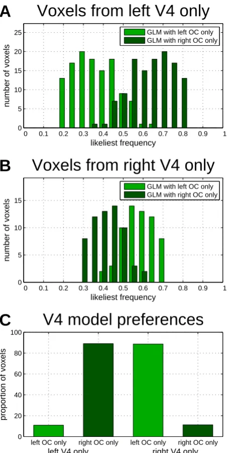
We present model selection results using histograms of likeliest frequencies (LF) across voxels from left and right V4, as defined by the localizer analysis. As can be seen, mod-elling only right OC (GLM III-r) makes a better model in left V4 (see Figure 5A) and modelling only left OC (GLM III-l) is performing better in right V4 (see Figure 5B) meaning that orientation pop-out processing is contra-lateralized (see Figure 5C). This is consistent with the fact that contents of the left visual hemifield are neurally processed in the right visual cortex and vice versa (Van Essen et al., 1992) and shows that model selection is capable of detecting anatomically plausible lateralization effects.
For comparison purposes, we have also performed all nested model comparisons (1st, 3rd and 4th model space) using conventional GLM techniques, i.e. omnibus F-tests on the additional regressors. These results are provided in the supplementary online material (see Supplementary Figure S1 and Table S1). Note that this type of classical model selection cannot be employed for non-nested model comparison (2nd model space).
0 0.1 0.2 0.3 0.4 0.5 0.6 0.7 0.8 0.9 1 0
5 10 15 20 25
likeliest frequency
number of voxels
Voxels from left V4 only
A
GLM with left OC only GLM with right OC only
0 0.1 0.2 0.3 0.4 0.5 0.6 0.7 0.8 0.9 1 0
5 10 15
likeliest frequency
number of voxels
Voxels from right V4 only
B
GLM with left OC only GLM with right OC only
left OC only right OC only left OC only right OC only 0
20 40 60 80 100
left V4 only right V4 only
proportion of voxels
[image:24.595.179.406.74.524.2]V4 model preferences
C
5
Validation: simulated data
We additionally validate the cvBMS approach using simulated fMRI data. We place these simulations after the empirical validation, because we want to generate realistic fMRI sig-nals and thus use one of the model spaces that were explained in the previous section and already applied to empirical fMRI data. We perform two simulations and investigate certain properties of the cvLME criterion in order to demonstrate that the cvBMS ap-proach is an appropriate tool for model selection. We only focus on the performance of the cvLME on the first level and not on the validity of RFX BMS at the second level since this latter part of the technique has already been validated (Stephan et al., 2009; Penny et al., 2010).
First, as model selection serves to infer the most likely model given the data, it should be capable of identifying true models – something which we do not know when analyzing empirical data, but which we can control in simulation-based validation. We therefore investigate the capability of the cvLME to identify the GLM that certain data were gen-erated with. We analyze this while varying between-session variance of the true parameter values, because the cvLME assumes stationarity of model parameters across recording sessions. This means that model selection performance is expected to decrease as non-stationarity across sessions increases. For this simulation, we use the three non-nested models from the 2nd model space that represent different ways of how experimental factors can be described.
5.1
1st simulation: influence of between-session variance
5.1.1 Methods
The model space consists of a categorical model (GLM I) which models all conditions
of the 4×4 design using 16 regressors, a linear-parametric model (GLM II) which puts
all trials into one regressor and encodes orientation contrast on the left and right visual hemifield as two parametric modulators and a nonlinear-parametric model (GLM III) in which the parametric modulators are a nonlinear function of orientation contrast. For the purpose of this simulation, movement parameters and implicit baseline were removed from the design matrix in each model (see Figure 6A).
From the first model, we extract the covariance matrix V as computed by SPM during
model estimation in order to induce the same temporal auto-correlation structure into
all data. For each model, we extract the design matrix X as generated by SPM during
model specification in order to simulate realistic fMRI signals. Both X and V describe 5
sessions of fMRI recording. Synthetic data is then generated as follows. First, true regression coefficients are drawn using the relation
βij =xj+yij
xj ∼N(0, σ2v)
yij ∼N(0, σ2s)
where i and j index session and parameter respectively, σ2v represents the voxel-to-voxel
variance andσ2
s represents the session-to-session variance. In other words, we are working
with regionally specific effects which are zero mean across all realizations (Friston et al., 2002a) and spherical covariance matrices on the regression coefficients (Penny, 2012).
The sampled parameters imply a certain true signalXβ and induce a certain signal
vari-ance var(Xβ). A residual or scan-to-scan variance σ2 is chosen such that var(Xβ)/σ2 =
SNR for a desired signal-to-noise ratio (SNR).
Second, simulated data is generated by sampling zero-mean Gaussian observation noise
according to the relation ε ∼ N(0, σ2V) and then adding the random noise to the true
signal to get a measured signal y=Xβ+ε.
In our simulation, we set σ2
v = 2.5 and SNR = 4.5 (which approximately correspond to
the median values 2.67 and 4.57 observed in the SPM template data set3) while
between-session variance σ2s is varied from 0.25 to 5 in steps of 0.25.
For each level ofσ2
s,N = 10,000 data sets are generated using a true model which results in
Nsim =N×20 = 200,000 simulations per model. Then, for each data set from each model,
we calculate the cvLME using each model which gives rise to Nsim×3×3 = 1,800,000
cvLMEs. Performance of cvLME is evaluated based on average model differences and the ability to recognize the true model.
3These data were first published as a study on repetition priming (Henson et al., 2002), previously used
5.1.2 Results
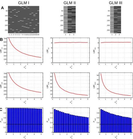
The results from this simulation are shown in Figure 6. Average log Bayes factors (LBF)
in favor of the true model and proportions of correct model selections (Pcorr) are plotted as
a function of the between-session varianceσ2
s. Note that σ2s is proportional to the squared
coefficient of variation of the regression coefficients across sessions CV2 = (σs/h|βj|i)2
and therefore can be seen as a measure of non-stationarity.
First, GLM I can be detected as the generating model with an overwhelming precision of 99.18 % (see Figure 6D, left). This is due to the fact that this model differs strongly from the other two models which in turn only differ from each other in small details. Additionally, GLM II and GLM III make very special assumptions about the signal as a function of orientation contrast while GLM I can account for more diverse activation patterns across experimental conditions.
Second, GLM II and GLM III can be reliably distinguished from each other, but less reliably selected against the other model. The reason for this is that true signals generated using GLM II or GLM III can also be identified by GLM I due to its higher flexibility. This means that GLM I can only be ruled out based on a complexity disadvantage. Still, detecting GLM II and GLM III as generating models works at acceptable accuracies of 75.06 % and 73.77 % (see Figure 6D, middle and right).
To our knowledge, the session-to-session variance (here:σ2
s = 0.25, . . . ,5) is almost always
lower than the voxel-to-voxel variance (here:σv2 = 2.5) in real fMRI data which is why we
1 2 3 4 5 6 7 8 9 10111213141516 50 100 150 200 250
GLM I
A
1 2 3 50 100 150 200 250
GLM II
1 2 3 50 100 150 200 250
GLM III
0 1 2 3 4 5 0 100 200 300 400 500 600 700
s2
LBF
I,II
B
0 1 2 3 4 5 0 100 200 300 400 500 600 700
s2
LBF
I,III
0 1 2 3 4 5 0 2 4 6 8 10
s2
LBF
II,I
0 1 2 3 4 5 0 10 20 30 40 50 60 70
s2
LBF
II,III
0 1 2 3 4 5 0 2 4 6 8 10
s2
LBF
III,I
0 1 2 3 4 5 0 10 20 30 40 50
s2
LBF
III,II
0 1 2 3 4 5 0 0.2 0.4 0.6 0.8 1
s2
Pcorr
C
0 1 2 3 4 5 0 0.2 0.4 0.6 0.8 1
s2
Pcorr
0 1 2 3 4 5 0 0.2 0.4 0.6 0.8 1
s2
[image:28.595.82.516.75.528.2]Pcorr
5.2
2nd simulation: influence of regressor correlation
5.2.1 Methods
We want to systematically study how model selection performance is influenced by shared variance between a model’s regressors and another regressor that might be added or not added to the model. To this end, we take the design matrix of the linear-parametric model (GLM II, null model) and use its parametric modulators to create a more complex model (GLM II+, full model). Ignoring movement parameters and the implicit baseline, GLM II has three regressors (see Figure 7A): an onset regressor encoding orientation contrast
events (x1), a parametric modulator for left OC (x2) and a parametric modulator for
right OC (x3). Then, GLM II+ has an additional artifical regressor (x4) that is given by
x4 = cos(α)xm+ sin(α)xo
xm = 1
2(x2+x3)
x2 ⊥xo ⊥x3
where xm is the mean of x2 and x3 and xo is a regressor that is orthogonal to x2 and
x34. In other words, we form x4 as an average of a highly correlated regressor xm and
a completely uncorrelated regressor xo where α determines the weighting and thereby
controls how much variancex4 shares with x2 and x3. Note thatx2 and x3 as well asxm
and xo are normalized to unit vectors in order to avoid scaling effects.
Ifα is very high, x4 will be dominated by the orthogonal regressor so that its correlation
withx2 andx3will be very low. In the case thatα= 0°,x4 has a correlation of around 0.7
with x2 and x3 and a correlation of 1 with (x2+x3). Importantly, we will not investigate
this extreme case, because the design matrix of GLM II+ is colinear in this situation,
making it a redundant model that is to be avoided a priori. Instead, we vary α from 5°
to 90° in steps of 5° and analyze different properties of the selected model.
Like in the first simulation, the design matrixXand the covariance matrixV are extracted
from the estimated SPM models and describe 5 sessions of fMRI recording. Synthetic data
is then generated using the same procedure as before, again using σ2v = 2.5, but with a
fixed σ2
s = 1.25 which induces a ratio of between-voxel to between-session variance of 2
and a coefficient of variation for the regression coefficients of around 0.88. Together with the very subtle model difference of a single covariate regressor, this relatively low effect consistency was intended to make model comparison as hard as possible.
For each level ofα, we generate the correspondingx4, and for each of thesex4,N = 10,000
data sets are generated resulting in Nsim = N ×20 = 200,000 simulations per model
(SNR = 0.1). In anotherNsim= 200,000 simulations for each model (SNR = 10), the true
values of the common model parametersx2 and x3 are set to zero in order to investigate
specificity (when true values are zero) and sensitivity (when true values are not zero) of statistical tests later on. For all these simulations, cvLMEs are calculated and LBFs are used to define the selected and the rejected model in each simulation.
4In this implementation, x
5.2.2 Results
The results from this simulation are shown in Figure 7. The correlation ofx4 withx2 and
x3 is shown as a function of regressor angleα. Moreover, mean squared errors (MSE) for
the common model parameters x2 and x3 as well as sensitivity (true positive rate, TPR)
and specificity (true negative rate, TNR) of an omnibus F-test on the parametersx2 and
x3 are plotted against α.
The two models have three common parameters. The MSE describes the expected squared
deviations of estimated parameters from their true values across simulations. When α is
low and correlation is high,β2 and β3 are estimated closer to their true values when the
selected model is used compared to when the rejected model is used (see Figure 7C).
Intuively, this effect disappears with higher α. This confirms that even if the additional
regressor is not of interest in itself, selecting the correct model still improves the parameter estimation for regressors of interest.
The capability of selected models to more precisely estimate parameters of interest also carries over to the quality of statistical test based on these parameter estimates. The sensitivity or TPR is the probability that the null hypothesis is rejected, given that it is false, and the specificity or TNR is the probability that the null hypothesis is not rejected, given that it is true. In our case, null hypothesis and alternative hypothesis are given by
H0 :x2 =x3 = 0 and H1 :x2 6= 0 orx3 6= 0
which means that we are testing whether there is an effect of orientation contrast for at least one side of the visual field. We have simulations using both models, GLM II and
GLM II+, in which H1 is true (when parameters are drawn from distributions), as well
as simulations in which H0 is true (when parameters are set to zero deliberately).
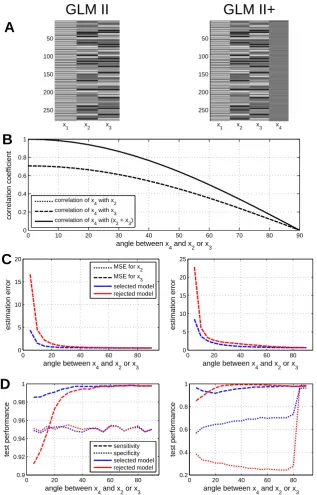
The simulation shows that sensitivity is reduced when the null model is true and the full model is used (see Figure 7D, left) and specificity is reduced when the full model is true and null model is used (see Figure 7D, right). The fact that the specificity suffers massively when the more complex model is true and the rejected model is used means that the F-test can be heavily invalidated by a large false positive rate (FPR) when models omit variables that would be required for sufficient explanation of the data. In contrast, the specificity does not decrease very much when the simpler model is true and the rejected model is used in our example. This is because the full model also contains all the regressors that are in the null model.
The problem of adding non-orthogonal regressors to a design matrix is well known among practitioners of GLM-based fMRI analysis (Andrade et al., 1999) and design orthogonality is commonly used to assess the amount of covariation between regressors (Ashburner et al., 2013, ch. 28). As is evident from the plots, differences in MSE as well as sensitivity
and specificity disappear when α is high, such that correlation with x4 becomes low.
50 100 150 200 250
x1 x2 x3
GLM II
A
50 100 150 200 250x1 x2 x3 x4
GLM II+
0 10 20 30 40 50 60 70 80 90 0 0.2 0.4 0.6 0.8 1
angle between x
4 and x2 or x3
correlation coefficient
B
correlation of x
4 with x2
correlation of x
4 with x3
correlation of x
4 with (x2 + x3)
0 20 40 60 80 0
5 10 15 20
angle between x
4 and x2 or x3
estimation error
C
MSE for x 2MSE for x
3
selected model rejected model
0 20 40 60 80 0 5 10 15 20 25
angle between x
4 and x2 or x3
estimation error
0 20 40 60 80 0.9 0.92 0.94 0.96 0.98 1
angle between x
4 and x2 or x3
test performance
D
sensitivity specificity selected model rejected model0 20 40 60 80 0.2
0.4 0.6 0.8 1
angle between x
4 and x2 or x3
[image:31.595.132.450.76.572.2]test performance
Figure 7. Simulation performance of nested model comparison. (A) Design matrices of the two models that were used in this simulation. Each column of the figure represents simulations in which the model at the top was the true model. (B) The additional regressor
of GLM II+ (x4) was manipulated so that it showed different degrees of correlation with
the two other regressors of interest (x2 and x3). (C) Mean-squared errors (MSE) for the
common parameters x2 and x3 when analyzing the data using the selected model (blue)
or the rejected model (red) as a function of their vector angle with x4. (D) Sensitivity
(dashed) and specificity (dotted) of an omnibus F-test on the common parametersx2 and
6
Discussion
We have introduced a model selection approach for constraining analysis approaches
when analyzing functional magnetic resonance imaging (fMRI) data using general linear
models (GLMs). We have demonstrated that cross-validated Bayesian model selection
(cvBMS) serves its intended purpose and that it is useful in practice. Usage of model assessment and model selection effectively removes uncertainty from GLM-based fMRI analysis, reduces model misspecification and thereby enhances the methodological quality of functional neuroimaging studies (Friston, 2009).
6.1
Model selection against first-level mismodelling
In functional neuroimaging, mismodelling can lead to suboptimal signal explanation and false statistical inferences. If just one model is estimated and no other modelling ap-proaches are considered, this can cause underfitting or overfitting so that researchers may
fail to reject null hypotheses that are false (false negatives). If many models are tested and
model choice is made by looking at significant results, this encourages p-hacking which
may lead researchers to reject null hypotheses that are true (false positives). Using model
selection, we can solve this problem. Model selection encourages multiple model estima-tion in order to avoid mismodelling, but bases the final model choice on objective criteria to avoid p-hacking. In our case, these objective criteria are how well a model fits the data (model accuracy), as a protection against underfitting, and how well it generalizes to new
data (negative model complexity), as a protection against overfitting.
The advantages of our approach are manifold: It represents a substantial advance over occasionally performed informal model selection using classical significance tests. It
prop-erly quantifies accuracy and complexity, it can handle arbitrary model differences and it
delivers voxel-wise optimal models. A disadvantage of the method is that cvLME maps
have to be calculated for each model separately without the possibility of only estimating one global model and then comparing within this model (Kherif et al., 2002; Penny and Ridgway, 2013). This is however alleviated by the technique’s computational efficiency and the modularity facilitated by the model-wise evidence calculation. Lastly, the possi-bility of using different GLMs for different parts of the brain can be easily implemented
by masking group analyses with the selected-model map (SMM) belonging to the model
that the group analyses were performed with. This means that second-level model es-timation is performed in all voxels, but second-level statistical inference is restricted to voxels where the corresponding first-level GLM is optimal.
such as posterior model probabilities (see Section 3.6) may allow to uncover individual variation in stimulus processing, e.g. in the context of visual receptive field mapping (Thirion et al., 2006; Kay et al., 2008b).
In the remainder of this section, we discuss issues relating to the theoretical aspects of our model quality measure as well as its practical application to empirical data and directions for future research.
6.2
Cross-validation and Bayesian model selection
In principle, cross-validation in a Bayesian context does not differ from cross-validation in a classical context. Parameters of interest are estimated from one (part of the) data set in order to test generalization of a model to another (part of the) data set. In fact, the cross-validated log model evidence (cvLME) is just the Bayesian analogue to the sum of out-of-sample log-likelihoods (oosLL) in Frequentist statistics, called the cross-validated log-likelihood (cvLL):
cvLL = S X
i=1
log p(yi|θˆ(∪j6=iyj))
cvLME = S X
i=1 log
Z
p(yi|θ)p(θ| ∪j6=i yj) dθ
Here, S denotes the number of sessions indicating S-fold cross-validation and the union
symbol ∪ signifies that parameters are estimated from several sessions as ML estimates
ˆ
θ(y) for cvLL or as posterior distributions p(θ|y) for cvLME. Whereas cvLL uses point
estimates and the likelihood function, cvLME accounts for the whole uncertainty about model parameters by using the marginal likelihood.
Cross-validation requires that data sets are drawn from the same source or population. This means that, in application to fMRI, the above formulas are based on the assump-tion of independence between recording sessions, mathematically implying that likelihood functions and marginal likelihoods factorize over parts of the data. Furthermore, cross-validating the log model evidence requires a certain degree of stationarity across sessions. Using simulations, we have investigated the influence of non-stationarity in the form of between-session variance on model parameters and found that the cvLME can accommo-date moderate stationarity violations.
Usually, cross-validation is considered to be a measure against overfitting. Since we are controlling for overfitting (and underfitting) already using the model evidence itself, our use of cross-validation has three other reasons: First, we wanted to avoid having to specify prior distributions on the model parameters. Second, we wanted to avoid approximations that originate from methods estimating hyperparameters like Empirical Bayes (Friston et al., 2008; Penny and Ridgway, 2013) or methods employing hyperpriors like Variational Bayes (Penny et al., 2003, 2005, 2007a). Third, and most importantly, we wanted to use the whole potential of the complexity penalty in the log model evidence along the following rationale.