Verifying Inevitability of Oscillation in Ring Oscillators Using the Deductive SOS-QE Approach

City, University of London Institutional Repository

Citation

: Ul Asad, H. and Jones, K. (2016). Verifying Inevitability of Oscillation in Ring

Oscillators Using the Deductive SOS-QE Approach. IEEE Design and Test, 33(5), pp. 35-43.

doi: 10.1109/MDAT.2016.2573588

This is the accepted version of the paper.

This version of the publication may differ from the final published

version.

Permanent repository link:

http://openaccess.city.ac.uk/15337/

Link to published version

: http://dx.doi.org/10.1109/MDAT.2016.2573588

Copyright and reuse:

City Research Online aims to make research

outputs of City, University of London available to a wider audience.

Copyright and Moral Rights remain with the author(s) and/or copyright

holders. URLs from City Research Online may be freely distributed and

linked to.

Verifying Inevitability of Oscillation in Ring Oscillators using

the Deductive SOS-QE Approach

Haz ul Asad

City University London

EC1V 0HB London UK

[email protected]

Kevin D. Jones

Plymouth University

PL4 8AA Plymouth, UK

[email protected]

Abstract

We present a deductive numeric-symbolic approach, using Sum of Squares programming (SOS) and Quantier Elimination (QE), and verify that a Ring Oscillator (RO) starts oscillating from almost all random initial voltages on its nodes.

1 Introduction

0 10 20 30 40 50 60 70 80 90 100 time(nano-seconds)

-1 0 1

v 1 ,v 2

(volts)

-0.8 -0.6 -0.4 -0.2 0 0.2 0.4 0.6 0.8 v₁(volts)

-1 0 1

v 2

(volts)

Figure 1: Dierent Representation of RO Oscillations

-0.8 -0.6 -0.4 -0.2 0 0.2 0.4 0.6 0.8 v₁(volts)

-1 -0.5 0 0.5 1

v 2

(volts)

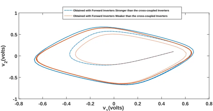
Obtained with Forward Inverters Stronger than the cross-coupled Inverters

Obtained with Forward Inverters Weaker than the cross-coupled Inverters

Figure 2: Parameters variation eect on the location of the Periodic Trajectory

Recently, there have been several eorts of using formal reachability analysis for the verication of the global inevitability property. Reachability tools model an RO as a continuous system, described by ordinary dierential equations (ODEs), and use set-theoretic simulations to see whether a target set is reachable from an initial set. The inevitability property is veried by using reachability analysis iteratively. Reachability suers from being of bounded-time nature, and since it relies on the over-approximate solutions of ODEs, is thus subjected to erroneous results. A survey of several such methods for can be found in [3]. In [1], the author showed convergence to the oscillation in an even stage RO with probability one. The author showed zero measure probability of the failure set using a cone argument. He further showed convergence to the desired limit cycle using reachability analysis. While the approach is comprehensive, it uses an expensive paper-pencil argument about the zero measure probability of the failure set. Secondly, they used the approximate but sound reachability computations, which is of bounded time nature and computationally very expensive.

−0.4 −0.2 0 0.2 0.4 −0.4

−0.2 0 0.2 0.4

S1 S2

−0.4 −0.2 0 0.2 0.4 −0.4

−0.2 0 0.2 0.4

S1

S2 Br

−0.4 −0.2 0 0.2 0.4 −0.4

−0.2 0 0.2 0.4

S1

S2 Br

−0.4 −0.2 0 0.2 0.4

−0.4

−0.2 0 0.2 0.4

AI>0

d(AI) dt <0

S1

S2 Br

Escape

Eventuality

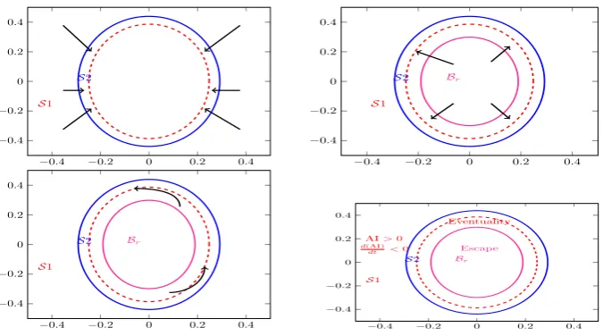
Figure 3: Verication Strategy: Dividing the convergence of trajectories to the dashed Periodic set into several Sub-tasks

based deductive approach to verify the inevitability of oscillations in ROs. We dene the verication task as a conjunction of several sub-properties whose verication is delegated to the existence of several Lyapunov-like certicates. Construction of these certicates can be posed as rst-order-formulas (FOFs) with quantiers (universal, existential). We use a sound numeric-symbolic approach, called SOS-QE, for the verication of these FOFs. This is basically using a numeric, yet computationally ecient, SOS programming technique for the certicates construction, followed by the symbolic validation of these certicates by the QE technique. A similar technique has been used for non-linear gain analysis in [5]. In [6], the author used SOS in HOL theorem prover to verify positivity of the universally quantied polynomials. Deductive and deductive-bounded approaches have been used for the inevitability verica-tion of a charge pump phase lock loop in [7]. To the best of our knowledge, this is the rst deductive approach for the solution of the research problem posed in [2]. Being deductive, our approach does not solve the ODEs and thus avoids the conservative approximation their solutions. Furthermore, once the inevitability property is veried, it stands veried for the innite time, unlike the bounded reachability analysis.

This paper is organized as follows: In Sec.II, we introduce the preliminaries of this paper. Sec.III illustrates verication of the inevitability of oscillation in RO. Experimental results are shown in Sec.IV. Sec.V concludes the paper.

2 Preliminaries

2.1 Verication Strategy

RO Model (Set of ODEs)

Almost Global Inevitability

Property

Dene Sub-properties

FOF formulation of Certicates

SOS Programming

Quantier Elimination

Property Veried No Conclusion Certicate(s)

In-validated, Check for other Struc-ture(s)

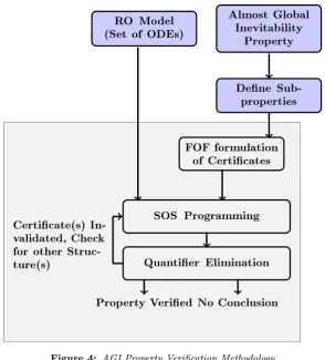
Figure 4: AGI Property Verication Methodology

eventually reaches S2 and stays there forever. Note that the set S2 is the area enclosed by the blue

circular closed path whereas S1 is the one outside it. In the second phase (top right), we show that

almost all trajectories in set Br, dened by the area enclosed by the magenta circular line, eventually

reaches to an annular region dened by the setS2\ Br. In the second stage, we also show that none of the

trajectories trap in the dead-set (from where RO fails to start). Finally, we show that all trajectories in the annular region (bottom left) converge to within an arbitrarily small distance of the desired periodic trajectory, shown by the dashed red circular path in Fig. 3. For each of these three sub-tasks, we dene three properties and state the AGI property as the conjunction of these three properties. Each of these sub-properties species the long term behavior of the trajectories of ROs in a specic sub-set of the state space which is veried by the existence of a certicate. These certicates, and their time derivatives, if exist, exhibit the characteristic of being positive (semi-positive) or negative (semi-negative) in their respective sub-sets. This scenario is depicted in the bottom right sub-gure of Fig. 3. As shown, we divide the space into three sub-sets;S1,S2, andBr. The dotted circle in the red shows the hypothetical

location of the periodic trajectory (Limit Cycle) in the state space. The trajectories of an RO exhibit dierent long term characteristics in these three dierent sub-sets. We use three dierent certicates called, the Attractive-invariance (AI), Escape, and Eventuality to verify dierent sub-properties. For illustration purpose, here we have depicted the positivity/negativity of the AI certicate in the setS1. The

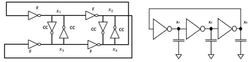
Figure 5: Two Dierent Topologies of Ring Oscillators. Left: Even Stage RO, Right: Odd Stage RO

over real polynomials. Verication of these FOFs is carried out using a numeric-symbolic technique of SOS programming and QE. The overall verication ow is shown in the Fig. 4. The existential quantication is solved by numerically nding dierent feasible certicates using SOS programming. To further validate these certicates, for their numerical imprecisions, symbolic analysis (QE) is carried out for each of the universally quantied formula. If a certicate is invalidated by the QE stage, a new search is made for a certicate(s) with a dierent structure this time. The output of our methodology results in either the AGI property being veried, or with no conclusion about its truthfulness, if a user-dened number of iterations have been exhausted.

2.2 Modelling of the Ring Oscillator

We model the RO shown in Fig. 5 as a polynomial continuous dynamical system. Let us denote byx,

the vector of node voltages at the outputs of inverters. The continuous dynamical system model of an RO is a tuple (X,Xinitial,U, f) whereX is a set of state variables interpreted overR, X =RX is the

set of all possible valuations of the variables, Xinitial ⊂ X is the set of initial conditions, U is the set

of parameters (to model circuit capacitance, resistance, transistor parameters) interpreted over Rwith

U =RU is the set of all possible parameter valuations, and

f :X × U → X (1)

is the vector eld characterizing the system. We assume that the vector eldf is a polynomial function

ofx∈ X called a polynomial vector eld. Let us denote byΦ(x0, t)the solution of equation

dΦ(X(t))

dt =

f(X, U), X(0) =x0∈ Xinit.

Denition 1 (Equilibrium state).

A statexe∈ X is called an equilibrium of the RO, if(xe) = 0.

Denition 2 (Attractive Invariance of a set).

A set XI is invariant i ∀x0 : x0 ∈ XI, Φ(x0, t)∈ XI for all t. It is called attractive invariant (AI) i

Denition 3 (Limit Cycle).

A set γ ⊂ X is called a Limit cycle, i ∀x0 : x0 ∈ γ, Φ(x0, T) = x0 forT >0, and for all0 < t < T,

Φ(x0, t)6=x0. This is an invariant set.

Denition 4 (Inevitability of the Limit cycle).

The Limit cycleγis said to be inevitable, i∀x0:x0∈ Xinitial, y∈γ, r >0, b∈R≥0,

lim

t→bkΦ(x0, t)−yk≤r (2)

Assumption 1.

In this work, we assume that the location ofγ in the state space is known.

For a practically feasible RO, there are states in Rn from where it fails to start and reaches the limit

cycleγ[1]. For example, Equilibrium is one such state from where an RO can not start. We call the set

of all such states the Dead set".

Denition 5 (Dead Set).

A set of states is called a dead set denoted byXdead, such that∀x0:x0∈ Xdead, limt→∞kΦ(x0, t)−xek=

0. Here xe is an equilibrium state.

Denition 6 (AGI of Oscillation in RO).

The Limit cycleγ⊂ X, is said to be Almost Globally Inevitable", i∀x0:x0∈ {X \ Xdead}, y∈γ, r >

0, b∈R≥0,

lim

t→bkΦ(x0, t)−yk≤r (3)

In this paper, we consider two dierent topologies of ROs, i.e., odd stage and even stage RO as depicted in Fig. 5. While we treat each individual node voltage as a state variable for the Odd stage RO, we use the strategy suggested in [1] for the even stage RO, and divide its operation into dierential and common modes. We denote the node voltages of the even stage RO by x(0, j) and x(1, j) for

j= 0,1...n−1. Herenis the number of stages. For the even stage RO in Fig. 5,x(0,0) =X1, x(0,1) =

X2, x(1,0) =X3, x(1,1) =X4. The voltagesx(0, j)andx(1, j)form the dierential pair whose dierential

component isx(0, j)−x(1, j), and the common mode component isx(0, j) +x(1, j). The even stage RO

while operating normally, has its oscillation manifested in the dierential mode, whereas the common mode settles to the constant zero value. If we assume that inverters are identical then, ∀j :j ∈[0, n−

1], ∀x: x∈ X such that x(0, j) =x(1, j), we have Φ(x, t) = xe as t → ∞. This means that the set

{x(0, j) = x(1, j),∀j : j ∈ [0, n−1]} ∈ Xdead. Similarly, for odd stage RO, if x1 = x2 = x3, then,

2.3 RO properties verication using Lyapunov-like Certicates

To verify the AGI of the limit cycle γ, we use several Lyapunov-like certicates in dierent subsets of

the state space of the RO, Fig. 3. To show attractive invariance of a set, a Lyapunov-like certicate has been presented in [8].

Lemma 1.

If there exist a polynomial with real coecientsV :X →_R, >0 and a minimumη >0 such that,

1. V(x)>0, ∀x∈Rn\0,

2. {V(x)≤1} ⊆ {q(x)≤η},

3. {V(x)≥1} ⊆ {∂V

∂x(x).f(x, u)≤ −},

then the set S2 := {V(x) ≤ 1} is an AI set for an RO with a vector eld given in Eq. 1, and it is

contained in the set{q(x)≤η}where q:X →R.

Proof. . See [8].

In the above Lemma 1, the set {q(x) ≤ η} is used for optimization purposes and the parameter

η is minimized so that this set contains the desired AI set S2 := {V(x) ≤ 1}. Inside the AI set S2,

trajectories can reach either, the dead setXdead, or to within a small distance of the limit cycleγ(shown

in dotted red in Fig. 3). Let us dene a set, Br=V(x)≤r, 0 < r <1 (shown in magenta in Fig. 3).

To show that trajectories starting in the set Br are not trapped in the dead set Xdead, and eventually

escape to the setS2\ Br, we introduce an Escape certicate.

Lemma 2.

For a compact setBr⊂ S2, if there is a dierentiable Escape certicate,E :X →R, such that

1. E(x) = 0∀x:x∈ Xdead,

2. E(x)>0∀x:x∈ Br\ Xdead,

3. ∂E

∂x(x).f(x, u)>0∀x:x∈ Br\ Xdead,

then∀x:x∈ {Br\ Xdead}, limt→∞x(t)∈ B/ r.

Proof. See [4, Chapter4].

To show that trajectories in the setS2\ Br eventually reach to within a close distance of the limit

cycleγ, we use the Eventuality certicate presented in [9]. Let us we have a setXLC, such that,ky−xk ≤

α, ∀x∈ XLC, y∈γ, α >0.

Theorem 1.

1. E(x)≤0 ∀x∈(S2\ Br)\ Xdead,

2. E(x)>0 ∀x∈Cl(∂S2\∂XLC),

3. ∂E

∂x(x).f(x, u)<0∀x∈Cl(S2\ XLC),

then for all initial conditionsx0∈ S2\ Br, the trajectoryx(t)satises,x(T)∈ XLC, for someT ≥0and

for allt∈[0, T],x(t)∈ X. Here Cl and∂ denote closure and boundary of a closed set respectively.

Proof. . See [9].

For the common mode of the even stage RO, we further show that common mode voltages settle down to zero in the steady state. We verify this using the Lyapunov certicate restated for the common mode in Th. 2.

Theorem 2.

For the continuous dynamical system with a vector eld given in Eq. 1, and with the state vector replaced byx={x(0,0) +x(1,0), x(0,1) +x(1,1), .., x(0, n−1) +x(1, n−1)}, let us we assume an invariant set

Xcom, which we call the common-mode state space. Note that this set is invariant due to the fact that

node voltages are bounded by the supply voltage. If there exist a Lyapunov certicateL:X →Rsuch

that,

L(x)>0, ∀x∈ {Xcom\ {0}}, L(0) = 0 (4)

∂L

∂x(x).f(x, u)<0, ∀x∈ {Xcom\ {0}} (5)

then the set{x= 0} is asymptotically stable, and∀x∈ Xcom, limt→∞Φ(x, t) = 0.

Proof. Similar to [4].

2.4 SOS Programming and QE

We formulate our verication methodology as a conjunction of several FOFs having polynomial equations, inequalities, quantiers{∀, ∃}and boolean operators{∧, ∨, ¬, →, etc}. There are algorithms that can

in principle generate quantier free formulas from a universal-existential quantied FOF over the real elds (See [6] and the references therein). However, they are complex and only work for small academic problems. Showing positivity of a real polynomial, SOS uses a sucient but incomplete criterion of establishing the decomposition of the polynomial into a sum of squares of polynomials [10]. A sucient condition for a multivariate polynomialp(x)to be non-negative everywhere is that it can be decomposed

as a sum of squares of polynomials, i.e.,p(x) =Pm i=1p

2

innvariables with real coecients byPn. A subset of this set is the set of SOS polynomials innvariables

denoted bySn.

3 Verication of AGI of Oscillation in RO

3.1 Formulation of the Verication problem

We formulate the verication of the AGI property as the conjunction of dierent sub-properties, corre-sponding to the three sub-gures in Fig. 3, dened below.

Property 1.

∀x(0) :x(0)∈ S1, limt→b x(t)∈ S2, b∈R≥0.

Property 2.

∀x(0) :x(0)∈ Br, limt→∞(x(t)6∈ Xdead ∧ x(t)∈ S2\ Br).

Property 3.

∀x(0) :x(0)∈ S2\ Br, limt→b ky−x(t)k ≤α, y∈γ, b∈R≥0, α >0.

We dene a fourth property characterizing the common mode behavior of the even stage RO in the invariant setXcom.

Property 4.

∀x(0) :x(0)∈ Xcom, limt→∞ x(t) = 0.

If we denote the almost global inevitability property byϕ, Property.1 byϕ1, Property.2 byϕ2, Property.3

byϕ3, and Property.4 byϕ4, thenϕ=ϕ1∧ϕ2∧ϕ3, for odd stage RO, and , ϕ=ϕ1∧ϕ2∧ϕ3∧ϕ4,

for even stage RO. A trajectoryx(t)of the odd stage RO satisesϕ, i, it satisesϕ1 inS1,ϕ2 inBr,

andϕ3in S2\ Br,i.e.,

∀x:x∈ X, x|=ϕ ⇐⇒ (x|=ϕ1 ∀x:x∈ S1) ∧(x|=ϕ2 ∀x:x∈ S2) ∧(x|=ϕ3∀x:x∈ S2\ Br).

Similarly, for en even stage RO,

∀x:x∈ X, x|=ϕ ⇐⇒ (x|=ϕ1∀x:x∈ S1) ∧(x|=ϕ2∀x:x∈ Br)∧(x|=ϕ3∀x:x∈ S2\Br)∧(x|=

ϕ4∀x:x∈ Xcom).

3.2 SOS-QE approach to verify AGI of oscillation

by the following FOF.

ψ0:=∃pP :ψ1

ψ1:=∀xX :ψ2

ψ2:=

     

(x6= 0 =⇒ V(p, x)>0)∧

{(1−V(p, x)≥0) =⇒ (η−q(x))≥0} ∧ {(V(p, x)−1≥0) =⇒ (∂V

∂x(p, x).f(x, u)≤ −)}      

Herep∈ Prepresents the coecients space of the certicateV. A sucient condition for the verication

of propertyϕ1is stated in the following theorem,

Theorem 3.

If there is a feasible certicate V(x), fullling the conditions in Lemma. 1, then,(x|=ψ0 ⇐⇒ x |=

ϕ1), ∀x(0)∈ S1, andS2 =V(x)≤1.

Following the suciency conditions in Th. 3, we verify ϕ1 using the mixed SOS-QE approach. We

start with a SOS program searching for the AI certicate V(x)such that it satises the conditions in

Lemma. 1. Note that every condition on V(x) in Lemma. 1 is a positivity/negativity condition which

can be formulated as a SOS condition. Furthermore, we need these conditions to be satised in dierent sets which is encoded using a sound mathematical technique called the S-procedure [10]. A SOS program incorporating these conditions is given below.

minimize η

subject to

(i) V(0) = 0,

(ii)      

V(x)−−Pn k=1s

k

1(x)gk(x)      

∈ Sn,

(iii)      

(η−q(x))−s2(x)(1−V(x))

     

∈ Sn,

(iv)      

(−−∂V

∂x(x).f(x, u))−s3(x)(V(x)−1)−

Pn

k=1s

k

4(x)gk(x)−P m j=1s

j

5(x)aj(u)      

∈ Sn,

∀x∈ X,{sk1, s2, s3, sk4, s

j

5} ∈ Sn, ∀k∈ {1, .., n}, ∀j∈ {1, .., m}, >0, η >0.

HereV(x), sk1, s2, s3, sk4, s

j

5, are polynomials of degreed.

In this SOS program, constraint (ii) enforces positive deniteness on the certicate V(x) by

X ={x∈ Rn :gk(x)≥0, fork ∈ {1, .., n}}. Constraint (iii) ensures that {V(x)≤1} ⊆ {q(x)≤η}.

Constraint (iv) incorporates the set inclusion {V(x) ≥ 1} ⊆ {∂V

∂x.f(x, u) ≤ }. This constraint also

ensures that parametersubelong to the set, {aj(u)≥0, for j ∈ {1, .., m}}. The above SOS program,

if feasible, returns a certicate of attractive invariance V(x)with its parameters p∈ P xed within a

limited numerical precision. We further verify the validity of this certicate using symbolic QE. Note that in QE, coecients are represented in Qn. Using QE, we check the truth value of the negation of

the formula ψ1, since the existential quantier has already been eliminated by the SOS program. On

refutation of¬ψ1, we conclude,(x|=ϕ1 ⇐⇒ x|=ψ0), ∀x∈ S1. If either the SOS program is infeasible

for a certicateV(x), or the QE tool returns a true valuation for the formula¬ψ1, we repeat the process

by increasing the degree of the certicateV(x). If we still can't get the desired certicate, we conclude

inconclusiveness about the truth value ofϕ1.

4 Experimental Evaluation

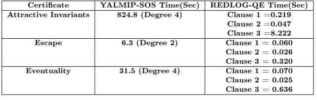
We used a degree-7 least-square polynomial model characterizing the input-output non-linear behavior of an inverter. We obtained this approximation of the inverter model by running MATLAB simulation using the Schichman-Hodges MOS transistor models. Note that, in this model, we take into account the eect of transistor widths/lengths on the slope of the inverter output. We used YALMIP [11] solver within MATLAB for SOS programming, and REDLOG [12], for QE on a 2.6 GHZ Intel Core i5 machine with 4 GB of memory. For an odd RO, we were able to compute a degree-4 AI certicate. The AI set, marked by the level set V(x)≤1, is shown in the Fig. 6. Inside the AI set, we showed trajectories escape the

set V ≤r, by computing a degree-2 Escape certicate. Similarly, the convergence of the trajectories to

within a small distance of the limit cycle has been shown by computing a degree-4 Eventuality certicate in the set {V ≤ 1∧V ≥ r}. Time taken by the SOS solver to compute these certicates is listed in

the second column of Table. 1. Verication of these certicates in REDLOG, given its ability of how large a formula it can handle, has been divided into the verication of the individual clauses of the FOFs beneting from its disjunctive normal form (DNF). Since we were interested in the negation of FOFs in the DNF, we veried whether each clause was false". The verication times of the QE are listed in the third column of Table. 1. For AI and Escape certicates, REDLOG successfully veried the negation of their universally quantied FOFs. A time-out was reported by the REDLOG tool for all clauses of the eventuality FOF of the odd RO. The reason for these time-outs is the set, an intersection of two level curves of the AI certicate, that puts an additional burden on the solver resulting in its time out. To overcome this issue, we instead, conservatively over-under approximate the set {V ≤1∧V ≥r}, by a

-1 -0.5 0 0.5 1

V

1

-1 -0.5 0 0.5 1

V 2

Figure 6: ODD RO AI Set, {r <=V <= 1}: Annular region between Solid green plots, Trajectories: Dashed plots

Certicate YALMIP-SOS Time(Sec) REDLOG-QE Time(Sec) Attractive Invariants 824.8 (Degree 4) Clause 1 =0.219

Clause 2 =0.047 Clause 3 =8.222 Escape 6.3 (Degree 2) Clause 1 = 0.060

Clause 2 = 0.026 Clause 3 = 0.320 Eventuality 31.5 (Degree 4) Clause 1 = 0.070 Clause 2 = 0.025 Clause 3 = 0.636

Table 1: ODD RO Inevitability Verication Time

the set{V ≤1∧V ≥r}. Note that this conservatism is to approximate the annular set{V ≤1∧V ≥r}

and does not add to the overall conservatism of our methodology.

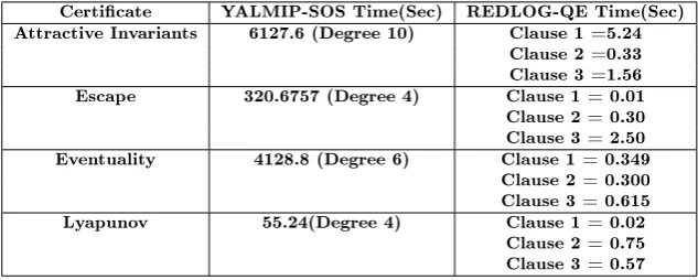
Similarly, for even stage RO, we computed a degree-10 AI, a degree-4 Escape, a degree-6 Eventuality and a degree-4 Lyapunov certicate. Computation times are given in Table. 2 and the AI set is shown in Fig. 7.

Though verifying the property, using SOS-QE approach, needs user input, it oers a comparable computation time to [1]. They have reported approximately 22000 seconds for the complete verication of the even stage RO, whereas our accumulative time for the even stage RO is approximately 6500 seconds. Even if we add the time of all the instances for which we got an infeasible certicate, our computation time is still not more than half of what has been reported in [1]. This is in addition to our methodology being less conservative and applicable to innite horizon.

5 Conclusion

x(0,0)- x(1,0)

-2

-1.5

-1

-0.5

0

0.5

1

1.5

2

x(0,1)-x(1,1)

-2

-1

0

1

2

Figure 7: Even RO AI Set,{r <=V <= 1}: Annular region between Solid green Plot, Trajectories: Dashed

Certicate YALMIP-SOS Time(Sec) REDLOG-QE Time(Sec) Attractive Invariants 6127.6 (Degree 10) Clause 1 =5.24

Clause 2 =0.33 Clause 3 =1.56 Escape 320.6757 (Degree 4) Clause 1 = 0.01 Clause 2 = 0.30 Clause 3 = 2.50 Eventuality 4128.8 (Degree 6) Clause 1 = 0.349

Clause 2 = 0.300 Clause 3 = 0.615 Lyapunov 55.24(Degree 4) Clause 1 = 0.02

Clause 2 = 0.75 Clause 3 = 0.57

Table 2: Even RO Inevitability Verication Time

References

[1] Chao Yan, Mark R Greenstreet, and Suwen Yang. Verifying global start-up for a Möbius ring-oscillator. Formal Methods in System Design, 45(2):246272, 2014.

[2] Kevin D Jones, Jeha Kim, and V Konrad. Some real world problems in the analog and mixed signal domains. In Designing Correct Circuits, 2008.

[3] Mohamed H Zaki, Soène Tahar, and Guy Bois. Formal verication of analog and mixed signal designs: A survey. Microelectronics Journal, 39(12):13951404, 2008.

[4] Hassan K.Khalil. Nonlinear Systems. Prentice Hall, third edition, 2002.

[5] Hiroyuki Ichihara and Hirokazu Anai. An SOS-QE approach to nonlinear gain analysis for polyno-mial dynamical systems. Mathematics in Computer Science, 5(3):303314, 2011.

[7] Haz Ul Asad and Kevin D Jones. Verifying inevitability of phase-locking in a charge pump phase lock loop using sum of squares programming. In Design Automation Conference (DAC), 2015 52nd ACM/EDAC/IEEE, pages 295300. ACM, 2015.

[8] Weehong Tan. Nonlinear Control Analysis and Synthesis using Sum-of-Squares Programming. PhD thesis, University of California, Berkeley, 2006.

[9] Stephen Prajna and Anders Rantzer. Convex programs for temporal verication of nonlinear dy-namical systems. SIAM Journal on Control and Optimization, 46(3):9991021, 2007.

[10] Stephen Prajna and Antonis Papachristodoulou. Analysis of switched and hybrid systems-beyond piecewise quadratic methods. In American Control Conference, 2003. Proceedings of the 2003, volume 4, pages 27792784. IEEE, 2003.

[11] Johan Lofberg. Yalmip: A toolbox for modeling and optimization in matlab. In Computer Aided Control Systems Design, 2004 IEEE International Symposium on, pages 284289. IEEE, 2004.