City, University of London Institutional Repository
Citation
:
Witzke, V., Silvers, L. J. and Favier, B. (2016). Evolution of forced shear flows in
polytropic atmospheres: A comparison of forcing methods and energetics. Monthly Notices of
the Royal Astronomical Society, 463(1), pp. 282-295. doi: 10.1093/mnras/stw1925
This is the published version of the paper.
This version of the publication may differ from the final published
version.
Permanent repository link:
http://openaccess.city.ac.uk/15186/
Link to published version
:
http://dx.doi.org/10.1093/mnras/stw1925
Copyright and reuse:
City Research Online aims to make research
outputs of City, University of London available to a wider audience.
Copyright and Moral Rights remain with the author(s) and/or copyright
holders. URLs from City Research Online may be freely distributed and
linked to.
Evolution of forced shear flows in polytropic atmospheres:
A comparison of forcing methods and energetics
V. Witzke
1?, L. J. Silvers
1and B. Favier
21Department of Mathematics, City University London, Northampton Square, London, EC1V 0HB, UK
2Aix Marseille Univ, CNRS, Cent Marseille, IRPHE, Marseille, France
3 August 2016
ABSTRACT
Shear flows are ubiquitous in astrophysical objects including planetary and stellar interiors, where their dynamics can have significant impact on thermo-chemical processes. Investigat-ing the complex dynamics of shear flows requires numerical calculations that provide a long time evolution of the system. To achieve a sufficiently long lifetime in a local numerical model the system has to be forced externally. However, at present, there exist several different forc-ing methods to sustain large-scale shear flows in local models. In this paper we examine and compare various methods used in the literature in order to resolve their respective applicabil-ity and limitations. These techniques are compared during the exponential growth phase of a shear flow instability, such as the Kelvin-Helmholtz (KH) instability, and some are examined during the subsequent non-linear evolution. A linear stability analysis provides reference for the growth rate of the most unstable modes in the system and a detailed analysis of the en-ergetics provides a comprehensive understanding of the energy exchange during the system’s evolution. Finally, we discuss the pros and cons of each forcing method and their relation with natural mechanisms generating shear flows.
Key words: methods: numerical – stars: interiors – hydrodynamics – instabilities –
turbu-lence.
1 INTRODUCTION
The relative difficulty of observing most astrophysical shear re-gions, such as those in the Sun, in detail makes it imperative to use analytical and numerical techniques to shed light on the motions present there. Global-scale numerical calculations of stellar inte-rior dynamics is one approach to investigate the mechanisms main-taining differential rotation (Brun & Toomre 2002; Miesch et al. 2008). However, by using a global approach, such models can not resolve a large range of length-scales in its entirety and have to rely on artificially large transport coefficients or subgrid-scale models. Therefore, numerical investigations using a local approach, where only a small fraction of the object is simulated, can help to provide a more detailed description of the region of interest.
Previous studies of astrophysical flows looked at an assortment of different velocity profiles, depending on the problem and choice of boundary conditions. In the case of Keplerian motion, which is in-vestigated in the context of accretion discs, usually a linear velocity profile is assumed (e.g. Brandenburg et al. 1995; Hawley, Balbus & Winters 1999; Dubrulle et al. 2005; Silvers 2008). This type of shear profile does not require an external force to balance viscous
? E-mail:[email protected] (VW); [email protected]
(LJS); [email protected] (BF)
dissipation and instead they incorporate the velocity via a shearing-box approach (Goldreich & Lynden-Bell 1965; Narayan, Goldreich & Goodman 1987), where the velocity is instantaneously present. In contrast, some investigations of stellar shear flows have used polynomial functions, as for example in Tobias & Hughes (2004) and Cline, Brummell & Cattaneo (2003a) while other investiga-tions have utilized trigonometric funcinvestiga-tions to model the velocity field (see, for example, Hughes & Proctor 2013; Cline, Brummell & Cattaneo 2003b). Such velocity profiles have a non-vanishing gradient at the boundaries. In order to minimise the effect of the boundaries on the shear layer a hyperbolic tangent profile can be used (see for example Br¨uggen & Hillebrandt 2001; Hughes & To-bias 2001; Vasil & Brummell 2008).
Hyperbolic tangent profiles are commonly used in classical stud-ies of Kelvin-Helmholtz instability and turbulence. However, most local numerical studies of the turbulence transition in shear flows take the approach of an unforced flow (Caulfield & Peltier 2000; Smyth & Moum 2000; Smyth & Winters 2003), which results in a finite lifetime of an initially unstable background state due to its in-evitable viscous decay. However, astrophysical shear flows can be either transient features or be sustained over very long time-scales, where the physical mechanism maintaining the shear flow is usu-ally unknown. Incorporating a forcing into the numerical model has therefore two roles first to sustain the initial state, for which a linear stability analysis can be carried out, and second to model
MNRAS Advance Access published August 3, 2016
at City University, London on August 16, 2016
http://mnras.oxfordjournals.org/
the unknown physical processes responsible for the resulting flow in an astrophysical system. A variety of classical studies of shear driven turbulence exploit a method where a decoupled background shear flow is present (for example used by Holt, Koseff& Ferziger 1992; Jacobitz, Sarkar & van Atta 1997; Barker et al. 2012). This method requires a change of variables to incorporate a mean shear profile and does not allow for a back-reaction of the actual flow on the forcing. Whereas investigations of astrophysical shear flows exploit different methods to provide a sustained flow. For exam-ple in Miesch (2003), Vasil & Brummell (2008), and Silvers et al. (2009) a method to balance viscous dissipation by introducing an external force proportional to the viscous term is utilized. Another option that has been selected is the relaxation method (e.g. Prat & Ligni`eres 2013), which incorporates an external force propor-tional to the difference between the actual velocity profile and the target shear profile. Furthermore, studies focusing on magnetohy-drodynamical instabilities used forced shear flows in order to study magnetic buoyancy and its relevance to the formation of sunspots (Tobias & Hughes 2004; Brummell, Cline & Cattaneo 2002). To understand the role of a shear flow for magnetic field generation, several investigations on the interaction between a shear flow and initial weak structured magnetic fields have been conducted (Vasil & Brummell 2008; Miesch, Gilman & Dikpati 2007; Heifetz et al. 2015). In all cases however, the influence of the forcing method used on the evolution of the system has not been studied.
In this paper, a comparative analysis of different forcing methods is performed to understand how different forcings affect the non-linear evolution of the KH instability. The governing equations are given in Sec. 2 along with the formulation of the forcing methods and numerical methods used. Our comparison of the different forc-ing methods is presented in Sec 3, where the exponential growth regime is compared in Sec. 3.1 and the non-linear phase is pre-sented in Sec. 3.2.
2 THREE-DIMENSIONAL MODEL
Although a linear stability analysis is a powerful tool to investi-gate possible instabilities of shear flows in stellar environment as previously studied in Witzke et al. (2015), understanding the com-plex dynamics requires three-dimensional non-linear calculations. In order set up a system that initially remains comparable to a lin-ear stability problem, which has a non-evolving background state, external forcing is needed. The force aims to maintain the initial conditions corresponding to the equilibrium state as long as non-linear effects are negligible. Our purpose is to investigate whether different forcing methods provide a temporally evolving system, which shows the predicted linear evolution, and in what respect the non-linear evolution depend on the method used.
2.1 Governing equations, boundary conditions, and background state
We consider a three-dimensional domain of depthd, bounded by two horizontal planes located atz = 0 andz = 1, and periodic in both horizontal directions. The fluid is assumed to be an ideal monatomic gas with the adiabatic indexγ=cp/cv=5/3 and con-stant dynamic viscosityµ, constant thermal conductivityκ, constant heat capacitiescp at constant pressure, andcvat constant volume. The set of dimensionless differential equations we consider is:
∂ρ
∂t = −∇·(ρu) (1)
∂(ρu)
∂t = σCk ∇
2
u + 1 3∇(∇·u)
!
− ∇·(ρuu)
− ∇p+θ(m+1)ρzˆ +F (2)
∂T
∂t =
Ckσ(γ−1) 2ρ |τ|
2 + γCk
ρ ∇2T
−∇·(Tu) −(γ−2)T∇·u (3)
whereρis the density,uthe velocity field,T the temperature,θ denotes the uniform temperature gradient across the layer, and p is the pressure. In the dimensionless equations above, all lengths are given in units of the domain depthd. The temperature and den-sity are recast in units ofTtandρt, the temperature and density at the top of the layer, and we take the sound-crossing time, which is given by ˜t=d/[(cp−cv)Tt]1/2, as the reference time. There are two
dimensionless numbers in the set of equations above: the Prandtl number,σ=µcp/κ, which is the ratio of viscosity to thermal con-ductivity and the thermal dissipation parameterCk = κτ/(ρtcpd). The strain rate tensor in equation (3) has the form
τi j=
∂uj
∂xi +
∂ui
∂xj −δi j 2 3
∂uk
∂xk. (4)
A force termFin equation (2) aims to model external forces re-sulting from large-scale global effects (such as Reynold stresses associated with thermal convection in global-scale calculations for example) not included in our local approach. This force can sustain a shear flow when needed and is set to zero otherwise. The different forcings that we will consider are described in Section 2.2. For the basic state a polytropic relation between pressure and den-sity is taken. Due to the Schwarzschild criterion the fluid is stable against convection if the inequalitym>1/(γ−1)=1.5 holds. In this paper the polytropic indexmis always chosen such that the atmosphere is stably stratified. The boundary conditions at the top and the bottom of the domain are impermeable and stress-free ve-locity and fixed temperature:
uz=∂ux
∂z =
∂uy
∂z =0 at z=0 and z=1, (5)
T =1 at z=0 and T =1+θ at z=1. (6)
The dimensionless initial temperature and density profiles are of the form:
T(z)=(1+θz) (7)
ρ(z)=(1+θz)m. (8)
This basic state corresponds to an equilibrium state if the fluid is at rest.
In order to obtain a shear driven turbulent regime it is necessary to start with an unstable velocity profile. A hyperbolic tangent profile is assumed in order to model a localised shear layer in the middle or our domain that will minimize the effects of the boundaries. There-fore, we assume that an external force sustains the following initial background velocity profile
U0=(u0(z),0,0)T =U0tanh
z−0.5 Lu
!
ˆ
ex (9)
with a shear amplitudeU0 and a scaling factor 1/Lu that controls
the width of the shear profile. The boundary conditions introduced in equation (5) restrict the shear profile to values ofLuwhich will result in a low enough value of thez-derivative at the boundaries. Using this velocity profile the above basic state can still be regarded as an equilibrium state if viscosity is neglected. Some shear profiles for different widths are illustrated in Fig. 1.
at City University, London on August 16, 2016
http://mnras.oxfordjournals.org/
−1 −0.5 0 0.5 1 0
0.1
0.2
0.3
0.4
0.5
0.6
0.7
0.8
0.9
1
U
Z
L
u = 0.05
L
u = 0.0125
L
[image:4.595.52.273.102.379.2]u = 0.0085
Figure 1.Plots of initial shear flow profiles. Shear flow profiles with dif-ferentLuparameter, but with the same amplitudeU0 =1 are plotted. The
z-axis corresponds to the vertical dimension.
Our calculations are initialized by adding a small random tem-perature perturbation to the equilibrium state including the addi-tional shear flow given by equation (9). In order to evolve the system in time equations (1) - (3) are solved by using a hybrid finite-difference/pseudo-spectral code (see for example Matthews, Proctor & Weiss 1995; Silvers, Bushby & Proctor 2009; Favier & Bushby 2012, 2013, and references therein). For the linear stability calculations, the eigenvalue-problem formulated in Witzke et al. (2015) is numerically solved on a one-dimensional grid in thez -direction that is discretised uniformly, and this method is adapted from Favier et al. (2012).
When using direct numerical calculations to solve the system nu-merically over considerable iterations an issue concerning the mo-mentum conversation might appear, which is specific to the choice of stress-free boundary conditions (see discussion in Jones et al. 2011). Despite the fact that equation (2) together with the bound-ary conditions in equation (5) conserves the momentum a cumu-lative effect of truncation errors at each time step might lead to an unphysical change in momentum when integrating over a vast num-ber of time steps. We have checked that both momentum and mass is indeed conserved for all the calculations presented in this paper.
2.2 Forcing methods
We will compare three different methods to sustain an initial shear flow where we distinguish between methods that are static,i.e.the force term does not change throughout the calculation, and dy-namic forcing methods that might vary depending on the current flow. Furthermore, methods with a force applied to a localised re-gion have a local force whereas for global forcing methods the force term applies on the whole domain. The main goal is to find a
forc-ing method that does not significantly alter the characteristics of the linear phase of the evolution but allows to reach a quasi-steady non-linear state.
2.2.1 Viscous method
In order to balance the viscous dissipation associated with the ini-tial shear flow profile given by equation (9) the force
F=−σCk∇2U
0 (10)
is added to the RHS of equation (2). By applying this viscous forc-ing the initial state given by equations (7) - (9) is in equilibrium provided that viscous heating is neglected. This method has been broadly applied in forced shear flows to model the dynamics of the solar tachocline (e.g. Miesch 2003; Silvers et al. 2009). Note that this method only balances for the viscous diffusion of momentum associated with the target profile and does not depend on the actual non-linear solution. In that sense, the forcing can be considered to be local and static.
2.2.2 Perturbation method
Our second method, the perturbation method, was previously used by Holt et al. (1992); Jacobitz et al. (1997); Barker et al. (2012). For this method a slightly different set of differential equations is solved. A decomposition of the velocity,u=U0+u˜ into a
back-ground shear flow,U0, and the deviation from the background
pro-file ˜uenables the maintenance of a shear flow that is independent of the unstable perturbations. Note, the background velocity profile U0 has to be time independent and divergence free. Thus,
insert-ing the above decomposition into the momentum equation (2) we obtain
ρ∂
∂t( ˜u+U0) = − ∇p+θ(m+1)ρzˆ−ρ( ˜u+U0)·∇( ˜u+U0) +σCk
"
∇2( ˜u+U0) +
1
3∇∇·( ˜u+U0)
#
, (11)
since we assume that our background profile does not vary with time and in the flow direction, the time derivative ofU0and the term U0·∇U0vanish. In order to ensure that the background velocity is
not dissipated by viscosity the viscous term associated with it is dropped. The equation takes the form
ρ∂u˜
∂t = − ∇p+θ(m+1)ρzˆ−ρu˜·∇U0−ρU0·∇u˜ +σCk ∇2˜
u + 1 3∇(∇·u˜)
!
, (12)
such that effectively the differential equation for the velocity per-turbations only is solved. Here, the velocity perper-turbations, ˜u, are initially zero, but the background velocity is incorporated through the two advective terms involvingU0. By the same procedure the equations (1) and (3) become:
∂ρ
∂t = −∇·(ρu˜)−U0·∇ρ (13)
∂T
∂t =
Ckσ(γ−1) 2ρ |τ|
2 +Ckσ(γ−1)
2ρ
∂2U
0
∂z2 +
γCk
ρ ∇2T
−∇·(Tu˜) −(γ−2)T∇·u˜−U0·∇T, (14)
where the effect of the background velocity,U0, on the density and temperature is taken into account. Mathematically, the equations forU0+u˜ are the same as foruin the viscous method. Therefore,
at City University, London on August 16, 2016
http://mnras.oxfordjournals.org/
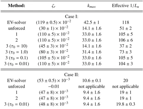
Table 1.Comparing the linear eigenvalue-solver results with those from non-linear calculations during the linear phase. For case I the shear am-plitude isU0 = 0.08 and 1/Lu = 118 such thatRi= 8×10⁻⁴. Taking Ck=8×10⁻⁵results in aPe=34. For case IIU0=0.041, 1/Lu=20 and Ck=1×10⁻⁴such thatRi=0.1 andPe=82.
Method: ζr kmax Effective 1/Lu
Case I:
EV-solver (119±0.5)×10−2 42.5±1 118
unforced (30±1)×10−2 14.1±1.6 51±2
1 (110±5)×10−2 33.0±1.6 105±5
2 (110±5)×10−2 33.0±1.6 106±6
3 (τ0=10) (45±3)×10−2 14.1±1.6 37±2
3 (τ0=1.0) (80±3)×10−2 31.4±1.6 73±3
3 (τ0=0.1) (105±5)×10−2 33.0±1.6 105±5
3 (τ0=0.01) (110±5)×10−2 33.0±1.6 104±3
Case II:
EV-solver (53±0.5)×10−3 10.6±0.1 20 unforced −0.01 not applicable not applicable
1 (47±8)×10−3 9.4±1.6 19±1
2 (47±8)×10−3 9.4±1.6 19±1
3 (τ0=0.01) (48±8)×10−3 9.4±1.6 19.8±0.3
both methods should give the same solutions, even if the approach and numerical implementation are significantly different.
2.2.3 Relaxation method
In the relaxation method, an external force ensures that the flow relaxes towards the initial profile on an arbitrary time-scaleτ0. We
define any quantity ¯f as
¯ f(z)= 1
NxNy Nx X
i=1 Ny X
j=1
f(i,j,z), (15)
where the overbar denotes that the quantity f is horizontally av-eraged, andNxandNyare the resolutions inx-direction and iny -direction respectively. The force for the relaxation method in the momentum equation depends on the horizontally averaged velocity ¯
ux(z) and is given by
F= ρ
τ0
(U0−ux¯ (z) ˆex), (16)
where ˆexis the unit vector in x-direction. For this method it is cru-cial to ensure that the forcing is aligned with the flow direction and does not depend on the velocity variation along this horizontal di-rection, which would otherwise correspond to a local small-scale force. A local forcing should be avoided, because it will suppress any instability and can lead to non-physical behaviour. The relax-ation method was used by Prat & Ligni`eres (2013) to model shear driven turbulence and provides the advantage of an adjustable back reaction on the actual mean flow. It is a global forcing (due to the averaged operator) and a dynamical forcing, because it depends on the actual flow.
3 COMPARISON OF THE FORCING METHODS
Investigating saturated flows on long time-scales requires an ex-ternal force to sustain a target velocity profile. Here we compare the effects of the different forcings presented in Section 2.2 on the
development of the shear instability. Our investigation is divided into two parts. We compare the linear regime of a shear instabil-ity in a two-dimensional framework in Section 3.1 and the non-linear regime is investigated in Section 3.2 using three-dimensional calculations. Here we first qualitatively examine two-dimensional slices and three-dimensional renderings of key quantities for diff er-ent forcing methods in Section 3.2.1, before we calculate the hori-zontally averaged velocity, turbulent Reynolds numbers and turbu-lent length in Section 3.2.2. A detailed analysis of the energy bud-gets is provided in Section 3.2.4, where the theoretical framework for the energy budgets is introduced in Section 3.2.3. The relation between the external work done by the forcing and the amount of dissipated energy by viscosity is analysed in detail in Section 3.2.5 and finally we summarize our findings for the saturated regime in Section 3.2.6.
3.1 Linear regime
Since the initial linear phase of shear flow instabilities is purely two-dimensional, which becomes evident from Squire’s theorem (Squire 1933), we focus here on calculations in a two-dimensional domain, which has a spatial resolution ofNx=512 andNz=480. The stability of a shear flow in a stratified atmosphere is charac-terized by the non-dimensional Richardson number,Ri. Using the general definition of the Brunt-V¨ais¨al¨a frequency given by
N2(z)= g ˜ T
∂T˜
∂z, (17)
where ˜T =T(Pt/P)1−1/γis the potential temperature, the minimum
value of the Richardson number,Ri, across the layer is defined as
Rimin = min
06z61 N(z)
2 , ∂
u0(z) ∂z
!2
= min
06z61
θ2L2
u(m+1)
m+1
γ −m
(1+θz) U0−u0(z)2/U02
, (18)
where the derivative of the background velocity profile, defined in equation (9), with respect tozcorresponds to a local turnover rate of the shear. In most cases the minimumRivalue is atz=0.5, but for some parameter choices with large temperature gradient,θ, and broad shear width the minimum is shifted towards greaterz. Here we consider unstable shear flows with a Richardson number less than 1/4 at a point in the domain. We do not consider shear instabilities triggered by thermal diffusion for which larger values ofRican be used (Dudis 1974; Zahn 1974; Ligni`eres et al. 1999). Because the 1/4 criterion is a necessary, but not sufficient, require-ment for instability we also solve the corresponding linear stability problem based on the approach used in Witzke et al. (2015) in ad-dition to conducting the non-linear calculations. For simplicity, the Prandtl number is fixed to be unity whereas the dimensionless ther-mal diffusivityCkis varied from 10−4to 10−5. Taking the previous
linear study by Witzke et al. (2015) into account, our parameters satisfy the following requirements: To ensure a stable stratification the polytropic index is set to bem=1.6, the amplitudeU0 of the
shear flow is chosen such that the Mach number in the middle of the domain remains less than 0.08, which avoids additional sta-bilisation by compressible effects. Furthermore, we take the initial P´eclet number, which we define as
Pe=4U0Lu
Ck , (19)
at City University, London on August 16, 2016
http://mnras.oxfordjournals.org/
to be much greater than unity to avoid a destabilizing effect caused by thermal diffusion. Note, that due to the definition ofU0andLu
in equation (9) a factor of 4 is needed to be consistent with the gen-erally used definition.
Here we want to compare two linearly unstable cases with distinct behaviour when no external forcing is included. An unforced case will decay if the instability grows on a larger time-scale than the viscous dissipation time-scale. Therefore, we consider two different cases corresponding to two different minimumRivalues. In case I we consider a very small value ofRi=8×10⁻⁴, such that the
sys-tem is unstable even without external forcing. Case II has a greater Ri=0.1 and greaterCkso that the system is unstable only if we in-troduce an external forcing. Without forcing, the initial shear flow diffuses quickly such that the Richardson number increases rapidly above 1/4 and no shear instability can be sustained. By considering these two different cases, we investigate how the forcing method used affects the development of a shear instability during the ex-ponential growth phase. Unforced calculations provide a reference for the system’s evolution without any external forces. All param-eters for case I and case II, the resulting linear growth rates, and the wave number for the most unstable mode for each method are summarised in Table 1 using both an eigenvalue solver and direct numerical calculations of unforced and forced cases.
The growth rates for the non-linear calculations are obtained by calculating
ζr=
dln<w>
dt =
1
<w> d<w>
dt , (20)
where the angle brackets denotes that any quantity fis volume av-eraged as follows
<f >= 1 NxNyNz
Nx X
i=1 Ny X
j=1 Nz X
l=1
f(i,j,l). (21)
In addition, we fit horizontally-averaged velocity profiles in the shear direction with a hyperbolic tangent profile as in equation (9) to estimate the shear width during the exponential regime. In order to find the most unstable wave number, which corresponds to the wave number with the most energy, the kinetic energy spectrum is calculated as
E(kx)=1 4
X
kx X
z ˆ
u(kx,z) ˆρu∗(kx,z)+ρˆu(kx,z) ˆu∗
(kx,z), (22)
where the hat symbol denotes the Fourier transform of the corre-sponding quantity and the star symbol denotes the complex conju-gate.
The growth rates for the viscous forcing, the perturbation method and the relaxation method (whereτ0 =0.01) are almost identical
for both case I and II. The growth rates achieved by these meth-ods in case II correspond to the growth rate calculated by using the EV-solver with a 12% relative error when taking the growth rate from the EV-solver as reference. For case I the error is 8%. The most unstable mode,kmax, in non-linear calculations is the same for the viscous- and the perturbation method. Note that the most unsta-ble wave number obtained by DNS is always slightly smaller than the one obtained from the eigenvalue solver, and more so for case I than for case II. This is due to a thinner shear width in case I, which is more affected by viscous dissipation, such that the instability is triggered when the shear profile is significantly broader. Therefore, kmaxdeviates for case I more than for case II, where the initial shear width is broader.
We now look at the effect of varying the relaxation time-scaleτ0in
the relaxation method. The instability develops always in the
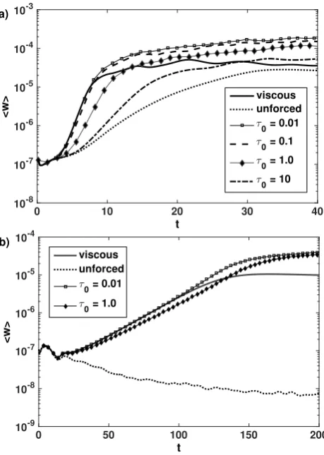
mid-dle of the domain and is visually similar to the instability observed by using either the viscous- or the perturbation method. The evolu-tion of<w>, for differentτ0parameters, for case I and case II is
shown in Fig. 2 and the growth rates of these runs are summarised in Table 1. For all cases the onset of the instability is not sensible to the chosen relaxation time-scaleτ0, but the growth rate decreases
with increasingτ0. This is expected since a smallerτ0 implies a
larger restoring force as soon as the averaged velocity profile dif-fers from the target equation (9). Therefore, for relaxation times that are larger the viscous dissipation might be unbalanced such that the initial state changes before an instability is triggered. The relaxation method leads either to the same instability or sus-tains an instability triggered by a smoother velocity profile, when the relaxation timeτ0is increased. To putτ0 in relation with
typ-ical dynamtyp-ical times the initial turnover time of the shear flow ts =Lu/U0 is calculated, which ists ≈0.1 for case I andts ≈1.2
for case II. Furthermore, the initial viscous time-scale,tµ=L2
u/µ, that accounts for the time on which the initially shear width is dis-sipated, gives another reference time. For case I the viscous time-scale istµ=0.9 and for case II it istµ=25. Note, that both time-scales represent initial time-time-scales given by the initial configura-tion and will change with time as the system evolves, especially in the saturated regime these times might be significant different from the initial values. So that a relaxation time greater than both the viscous and dynamical time-scale corresponds to a very weak back-reaction of the forcing to the change of the averaged velocity. Note thatτ0<1 means that the forcing relaxation is quicker than a
sound crossing time which is unlikely to occur in physical system. By varying the relaxation times,τ0, we investigate how to chose
an appropriateτ0with respect to the initial time-scales in order to
recover the linear instability dictated by the initial state and at the same time a saturated regime that evolves towards a quasi-static state.
As expected the numerical calculations using the viscous method and perturbation method lead to exactly the same result, because both methods are mathematically equivalent. Note however that the computational cost is slightly greater when using the perturbation method. In conclusion the viscous and perturbation method are the same, but the relaxation method shows different dynamics depend-ing on the relaxation time. If we are to understand which of these forcing methods is most suitable to model shear flows in stellar interiors it is essential to conduct a comparison for the non-linear evolution.
3.2 Non-linear phase
In order to investigate the non-linear evolution of a stratified shear flow a three-dimensional domain is crucial (Thorpe 1987), because after a Kelvin-Helmholtz instability three-dimensional instabilities are triggered (Peltier & Caulfield 2003). These secondary instabilities lead to a turbulent collapse of horizontal vortices, which is suppressed in a two-dimensional setup as discussed by Scinocca (1995). Therefore, to capture the effect of different forcing methods on the entire dynamics we now focus on three-dimensional calculations, which have a spatial resolution of Nx=256,Ny=256 andNz=360 .
To avoid confinement effects associated with the upper and lower boundaries, we focus on a case with a temperature gradientθ=5. In this case the instability is more likely to remain confined in a narrow central region as to minimize the importance of our particular choice of boundaries. The polytropic index is kept the same as in the previous section to ensure a stable stratification. A
at City University, London on August 16, 2016
http://mnras.oxfordjournals.org/
0 10 20 30 40
t
10-8
10-7
10-6
10-5
10-4
10-3
<w>
a)
viscous unforced
τ
0 = 0.01
τ
0 = 0.1
τ
0 = 1.0
τ
0 = 10
0 50 100 150 200
t
10-9
10-8
10-7
10-6
10-5
10-4
<w>
b)
viscous unforced
τ
0 = 0.01
τ
[image:7.595.322.524.90.714.2]0 = 1.0
Figure 2.The time evolution of the volume averaged vertical velocity, as defined in equation (21), for the two-dimensional calculations for case I in (a) and for case II in (b). Differentτ0parameters for the relaxation method
are used and compared to the viscous method and unforced calculations. The vertical velocity is displayed in logarithmic scale and t is given sound-crossing time.
parameter search was conducted to find combinations of the other parameters that lead to a finite spread of the unstable region. The dynamical viscosity is taken of order 10−4and the Prandtl number, σ=0.1, because low Prandtl number flows are more relevant for stellar interiors. The shear flow amplitude is set toU0 =0.2 and
we take 1/Lu=80 such thatRimin=0.003.
As discussed above, the viscous method and the perturbation method are equivalent, such that in the following, only results ob-tained with the viscous method are shown but we have checked that the calculations are indeed the same when using the perturbation method. Our study compares the resulting non-linear dynamics obtained by using the viscous method and the relaxation method. Furthermore, we discuss the effect of varyingτ0 in the relaxation
method and how does it compare with the viscous method, taken as reference.
3.2.1 Visualisation
In order to compare the flow evolution we start with a visualiza-tion of the vorticity at three different stages during the non-linear saturation. The first stage is the exponential growth phase, during which all forcing methods show a similar evolution, where the layer with non-zero vorticity spreads vertically. For the viscous forcing
Figure 4.The vertical velocity component w for three different forcing methods at several sound crossing times after saturation. In (a) the viscous method is used at ˜t≈40. In (b) the relaxation method is used withτ0=10
at ˜t≈40 and in (c) the averaged method is used withτ0=0.1 at ˜t≈38.
at City University, London on August 16, 2016
http://mnras.oxfordjournals.org/
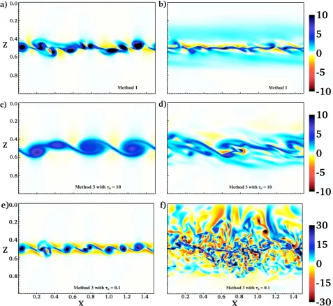
[image:7.595.48.278.101.424.2]Figure 3.The vorticity component perpendicular to the x-z-plane for different forcing methods at two different stages during the time evolution. The plots at the top (a), (b) show snapshots of two different times for the viscous method, where (a) is at ˜t=7.2, (b) at ˜t=40. The middle row (c) and (d) show the relaxation method withτ0=10 at ˜t=6.8 and ˜t=40, respectively. In (e) and (f) the relaxation method withτ0 =0.1 was used, where ˜t=12.3 in (e) and
˜
t=38 in (f).
and the relaxation method withτ0 1, this layer remains
signif-icantly smaller than for calculations where the relaxation method withτ0∼ O(1) is used. Note that the the viscous time-scale for this
case istµ≈1.5.
The second stage is chosen at a point when the instability starts to saturate and the fluid parcels overturn. In Fig. 3 the vorticity com-ponent perpendicular to the x-z plane for the viscous forcing, the relaxation method withτ0 =0.1 andτ0 =10 for the second and
third stage are plotted in the x-z plane at y=0.8. For the second stage the dynamics differ between the different forcing methods, which can be seen in Fig. 3 (a), (c) and (e). In Fig. 3 (a) small patches of strong positive vorticity are merging together into each other along a thin horizontal layer and a few small negative vorticity patches are present. In comparison, when using the relaxation method with
τ0=10 large billows of smaller positive vorticity occupy a
horizon-tal layer which is more extended in the vertical direction, see Fig. 3 (c). This can be explained by the smoother shear width, which is a consequence of the slow back-reaction of the forcing. Using a smallerτ0 leads to a greater vorticity amplitude than achieved by
the viscous method (see Fig. 3 (a) and (e), note the different color scales) while the spread of the instability remains similar. The third stage for the different methods is several sound crossing times after saturation, where the flow is evolving towards a quasi-static state. Comparing Fig. 3 (b), where the viscous method is used with Fig. 3 (d), and Fig. 3 (e), where the relaxation method with
τ0 = 10 andτ0 = 0.1 is used respectively, the main differences
are the vertical extent of the overturning region and the amplitude of the vorticity. Using a largerτ0 =10 leads to a similar situation
as for the viscous method which becomes evident when comparing Fig. 3 (b) and (d). In Fig. 3 (b) the layer is thin and shows elongated
at City University, London on August 16, 2016
http://mnras.oxfordjournals.org/
regions of strong positive vorticity, whereas in Fig. 3 (d) the region is significantly extended with small patches of strong positive and negative vorticity. A few larger regions are present further away from the middle of the domain. For the relaxation method with
τ0=0.1 a drastically different behaviour is observed, see Fig. 3 (f),
where the vorticity amplitude is much greater and the region where overturning is present is taking up almost the entire domain. In ad-dition, much more small scale turbulence occurs aroundz = 0.5. This can be explained by the form of the forcing used: The viscous method acts with a force, that is confined in a narrow region around the middle of the domain such that the instability can develop freely further away fromz=0.5. The relaxation method drives the fluid towards the target profile even far away from the middle of the do-main. This supports additional spread of the shear instability and triggers more turbulent motion. While it is worth mentioning that for the relaxation method withτ0=0.1 due to strong viscous
heat-ing convective motion is present in the upper half of the domain (which we checked by calculating the Brunt-V¨ais¨al¨a frequency), this dynamics will not be further discussed, as it is the result of the artificially low value ofτ0used in that case. Furthermore, we expect
[image:9.595.312.539.107.378.2]this unrealistic instability to disappear at lower Prandtl numbers. Fig. 4 shows contour plots of the vertical velocity in three dimen-sions at approximately 40 sound-crossing times, which is well af-ter the non-linear saturation. For the viscous method the patches of downwards and upwards motion form an alternating pattern along the x-direction where regions of the same velocity are arranged in small tubes that are extended along the y-direction, see Fig. 4 (a). Such a pattern is not present in Fig. 4 (b), where the relaxation method withτ0=10 is used. Here, the regions of the same velocity
form larger patches which are extended along the x-direction and changes sign along the y-direction. This indicates that a secondary instability which forms overturning billows along the y-direction is more dominating when the relaxation method with larger values of
τ0is used. For the relaxation method withτ0 =0.1, displayed in
Fig. 4 (c), the artificially strong forcing leads to an intense forward energy cascade and associated small-scale turbulent motions in the middle of the layer. The large-scale structures observed in the up-per part of the domain are convective cells resulting from the large central viscous heating.
When looking at the time evolution along Fig. 3 (a), (b) and the evolution along Fig. 3 (e), (f) a significant difference in the ampli-tude of the vorticity can be noticed. While for the viscous method the amplitude increases towards a peak during the saturation, Fig. 3 (a), and start to decrease afterwards, for the relaxation method the amplitude of the vorticity constantly increases and reaches a maximum after saturation, see Fig. 3 (b) and (f). This might be ex-plained by the form of the forcing: Because the relaxation method adjusts the magnitude of the force according to the mean flow, the strength of the force increases constantly and lead to more over-turning with time, whereas the force remains constant when using the viscous method, such that the overturning settles down after saturation. However, in order to check if this is indeed the case a more detailed analysis on the work done by the force and the total viscous dissipation is required, which is discussed in Section 3.2.4. Having compared the non-linear evolution for different forcing methods qualitatively we can conclude the following. The viscous method and the relaxation method withτ0 ∼ O(tµ) or larger
re-sult in similar, but still distinct, evolutions. Using a relaxation time
τ0 tµ but still greater than the dynamic time-scalets ≈ 0.06 leads to a very different non-linear dynamics with great mixing and possible non-physical behaviour leading to convection. Therefore, we conclude that, for the saturated regime, the initial viscous
time-0 0.2 0.4 0.6 0.8 1
Z
200 400 600 800 1000 1200 1400
Re
t
a)
viscous
τ 0 = 1.0
τ 0 = 10
0 0.2 0.4 0.6 0.8 1
Z
0 0.5 1 1.5 2
lt
b)
viscous
τ 0 = 1.0
τ 0 = 10
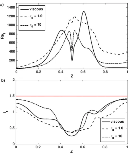
Figure 5.The turbulent Reynolds number and turbulent length-scales for three different forcings. In (a)Ret, as defined in equation (23), is plotted versus z and (b) showslt, where the red line indicates the horizontal extend of the domain.
scale, heretµ≈1.5, gives a reference time for the choice ofτ0and
the case withτ0=0.1 will be excluded from further analysis.
3.2.2 Horizontally averaged profiles
The system under consideration is stratified, such that most quanti-ties will change with depth,z, throughout the domain. Therefore, investigating horizontally averaged profiles with depth provides further insight in the system dynamics during the saturated regime. Let us first define a local turbulent Reynolds number as follows
Ret(z)=ρ¯(z)lt(z)urms(z)/(σCk), (23)
where ¯ρ(z) is the horizontally averaged density. Hereurms(z) is the root mean square of the fluctuating velocity averaged over the hor-izontal layers calculated as follows
urms(z)= 1 NxNy
Nx X
x=1
Ny X
y=1 q
(u(x,y,z)−U0(z))2, (24)
whereU0(z) is the target velocity profile as defined in equation (9). The turbulent length-scale is taken as
lt(z)=2π
R
E(k,z)/k dk
R
E(k,z)dk , (25)
wherek2 =k2
x+k
2
yis the horizontal wave number and the energy spectrumE(k,z) is averaged over horizontal layers such that it takes the form
E(k,z)=1 4
X
k ˆ
u(kx,ky,z) ˆρu∗(kx,ky,z)+ρˆu(kx,ky,z) ˆu∗(kx,ky,z).(26)
at City University, London on August 16, 2016
http://mnras.oxfordjournals.org/
0 0.1 0.2 0.3 0.4 0.5 0.6 0.7 0.8 0.9 Z
-0.2 -0.15 -0.1 -0.05 0 0.05 0.1 0.15 0.2 ¯
ux
viscous
τ 0 = 1.0
τ 0 = 10
[image:10.595.48.279.101.306.2]initially
Figure 6.The horizontally averageduxprofiles att ≈ 60 are shown for different forcing methods. Two differentτ0parameters are considered for
comparison.
The resulting Reynolds number variations with depth for the four different runs after 60 sound-crossing times is shown in Fig. 5 (a). It becomes evident that the flow for all four cases is very different at the late stage of the calculation. The viscous method is charac-terised by two regions above and below the middle of the domain, where the flow has high Reynolds numbers about 850 and 1300 respectively. The asymmetry is due to significantly denser fluid at the bottom of the domain. For the relaxation method withτ0=10,
these two regions are narrower and the maximal Reynold numbers are approximately 800 and 900. Forτ0 = 1.0 the region of high
Retis spread with two peaks very close toz=0.5. For these three methods a moderate turbulent flow confined in the middle is ob-tained. The corresponding turbulent length-scales, shown in Fig. 5 (b), reveal that for the three methods used the length-scales become less than 0.5 aroundz=0.5 and increase towrads the boundaries. Using the viscous method leads for this particular case to smaller turbulent length scales than using a relaxation method.
We now consider the horizontally averaged velocity profile ¯ux(z) shown in Fig. 6 at a time, ˜t, where the system evolves towards a quasi-static state. For all methods the shear profile is smoothed out. For the relaxation method ¯ux(z) remains a hyperbolic tangent pro-file, but for the viscous method a steep transition occurs around z = 0.5, which merges into a smoother region at the boundaries. This is caused by the different type of forcing: The force applied in the viscous method is solely defined by the shape of the target profile. Since the initial target profile has a thin width, the second derivative is large in this region, which causes a stronger forcing, compared to the outer parts of the domain. In contrast the relaxation method applies a force that depends on the deviation of the actual mean profile from the target profile, such a back reaction ensures the preservation of a hyperbolic tangent profile.
3.2.3 Theoretical framework for energy budgets
To get a more comprehensive insight on the processes involved when a linear shear flow instability saturates it is useful to track the evolution of the standard forms of energy during the transition
phase and beyond. Following the same procedure as used in Lan-dau & Lifshitz (1987) and Griffies (2004) we decompose the total energy into the kinetic energy,Ekin, internal energy,I, and gravita-tional potential energy,Epot, which in our case are given as
Ekin = 1 2
Z
V
ρu2dV (27)
I = cv
Z
V
TρdV (28)
Epot = −θ(m+1)
Z
V
ρzdV, (29)
where the volume integral is taken over the whole domain and the internal energy for an ideal gas is considered. Then, in order to understand the energy evolution with time, and to get more de-tailed insights into energy budgets, it is useful to derive the energy changes in our system using equations (1) - (3). The time derivative of the kinetic energy becomes
∂Ekin
∂t =
∂ ∂t 1 2 Z V
u·uρdV
!
(30)
= σCk
I
S
τ·u·nˆdS
| {z } =0
−σCk
Z
V
τi j
∂ui
∂xjdV
| {z }
ε
−1
2
I
S
|u|2ρu·ndSˆ
| {z } Ha
− Z
V u·∇pdV
| {z } Hp
+Z V
θ(m+1)ρw dV
| {z } Hρ
+Z V
u·FdV
| {z }
W = −ε− Ha− Hp+Hρ+W
whereSdenotes the volume surface,εis the positive viscous dissi-pation rate,Hais the change rate due to advection,Hpis the rate of work done by expansion and contraction,Hρdenotes the exchange rate with the potential energy due to density flux andWis the work done by external forcing. For the rate of change in the internal en-ergy we get
∂
∂tI =
∂ ∂t cv
Z
V TρdV
!
(31)
= cv
I
S
γCk∇T dS
| {z } Φtemp
+cv(γ−1)
Z
V u·∇pdV
| {z } Hp
+cv
Z
V
ρqdV
| {z }
ε = Φtemp+Hp+ε,
whereq=Ckσ(γ−1)|τ|2/2ρsuch thatεis due to viscous heating
andΦtempcorresponds to heat loss or gain at the surface,S. In the standard form, the changes in the gravitational potential energy are only due to the exchange of density flux as can be seen by taking the time derivative
∂
∂tEpot =
∂
∂t −
Z
V
θ(m+1)ρzdV
!
(32)
= θ(m+1)
I
S zρu·ndSˆ
| {z } =0
−θ(m+1)
Z
V
ρwdV
| {z } Hρ
=−Hρ.
Summing equations (30) - (32) yields the total energy change of the system
∂ ∂t
Ekin+Epot+I=W+ Φtemp− Ha, (33)
at City University, London on August 16, 2016
http://mnras.oxfordjournals.org/
Table 2.Time intervals of the different dynamical stages for the viscous forcing and relaxation method with two differentτ0.
Viscous Relaxation Method Stage: Method withτ0=1 withτ0=10
before instability 0<t<2.5 0<t<3.5 0<t<4.5 exponential growth 2.5<t<4.5 3.5<t<6.5 4.5<t<10
saturation 4.5<t<23 6.5<t<30 10<t<30 quasi-steady state t>23 t>30 t>30
which is only due to external forces, heat loss or gain at the sur-faces, and advection. Note, thatHa is negligible in our case, be-cause our system is closed and mass is conserved. It can be seen that viscous dissipation,ε, density flux,Hρ, and work done by expan-sion and contraction,Hpare exchanged between the kinetic energy and the potential energies. However, using the standard decompo-sition of energies it remains impossible to distinguish between re-versible and irrere-versible energy exchange between these three en-ergy budgets. In order to resolve this issue Winters et al. (1995) introduced a method to analyse the mixing behaviour of a turbu-lent flow, which can be used to track reversible and irreversible changes of different potential energies. This framework was further extended to compressible fluids by Tailleux (2013). For this method we decompose the gravitational potential energy of the system de-fined in equation (29) into two parts. One part is the so-called back-ground potential energy defined as
Eback=−θ(m+1)
Z
V
ρ?zdV, (34)
where theρ?is the adiabatically redistributed density. This defini-tion is also appropriate for a compressible fluid. Another part is the available potential energy
Eavail=−θ(m+1)
Z
V
(ρ−ρ?)zdV, (35)
which corresponds to the difference between the actual potential energy Epot and Eback. The available potential energy can be transformed into other types of energies, whereas the background energy can not be accessed and transformed in other types of ener-gies. Therefore, the background potential energy can be interpreted as the part of the total gravitational potential energy that corre-sponds to the lowest energy level that can be reached if the system is adiabatically redistributed. While a system is evolving the background potential energy can be only changed by irreversible processes. In our numerical calculations the background potential energy is obtained by taking the actual density distribution and sorting it in an ascending order, such that the highest density is at the bottom of the domain. In a similar procedure the internal energy can be decomposed into a background internal energy budget and an available internal energy budget, for a more detailed discussion see Tailleux (2013). However, for our purpose it is sufficient to analyse only the budgets for the gravitational potential energy in order to understand the mixing behaviour of the system.
3.2.4 Energy budgets from numerical calculations
The Kelvin-Helmholtz instability converts the kinetic energy that is available to the base horizontal shear flow into vertical fluctuations that need to overcome the stably-stratified atmosphere. The gravitational potential energy of the system is changed
0 10 20 30 40 50 60
1.5 2 2.5
3x 10
−4
a)
E kin
(t) / E
tot
(t=0)
viscous
τ
0 = 1.0
τ
0 = 10
0 10 20 30 40 50 60
0.607 0.608 0.609 0.610 0.611 0.612 0.613
b)
I (t) / E
tot
(t= 0)
viscous
τ
0 = 1.0
τ
0 = 10
0 10 20 30 40 50 60
0.392 0.3925 0.393 0.3935 0.394 0.3945 0.395 c)
t
E pot
(t) / E
tot
(t = 0 )
viscous
τ
0 = 1.0
τ
[image:11.595.44.278.134.209.2]0 = 10
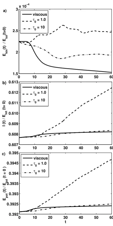
Figure 7.The total kinetic energy, internal energy and the gravitational po-tential energy evolution for viscous forcing and relaxation method by us-ing two differentτ0. In (a)Ekin(t)/Etot(t =0) is plotted with time, in (b)
I(t)/Etot(t = 0) and in (c) Epot/Etot(t = 0) is displayed, where all en-ergies are normalised by the initial total amount of the system’s energy
Etot(t=0)=195.81.
during this process. In addition, after saturation the fluid starts to overturn, and is mixed, where irreversible processes change the potential energy. Here we want to investigate how the forcing contributes to the different forms of energy in the system. Using the separate components responsible for the change in different energy budgets presented above and tracking the changes of the kinetic energy, internal energy and different gravitational potential energy budgets, we will discuss how the system behaves for different forcings. Below we distinguish between four stages of the system’s evolution that are: the time interval before the exponential growth of an instability, the exponential growth phase, the onset of
at City University, London on August 16, 2016
http://mnras.oxfordjournals.org/
0 10 20 30 40 50 60 −0.5
0 0.5 1 1.5 2 2.5 3 3.5x 10
−6
t Eavail
(t) / E
tot
(t=0)
viscous τ
0 = 1.0
[image:12.595.44.278.108.314.2]τ 0 = 10
Figure 8.The available gravitational potential energyEavail(t)/Etot(t=0) evolution for both the viscous forcing and relaxation methods by using two differentτ0.
saturation, and a fully saturated quasi-steady state. These stages are at different times for the three calculations that are discussed and can be found in Table 2.
Significant differences between the forcing methods become evident when following different energy budgets normalized by the initial value of the system’s total energy with time as shown in Fig. 7. In general the sum of the three energies is increasing due to the external work done by the forcing. For the viscous forcing the kinetic energy remains almost constant until the instability starts to grow at ˜t≈3, at that timeEkinbegins to decrease. The internal energy increases at an almost constant rate from the beginning of the calculation, which is due to viscous heating that extracts kinetic energy viaεin equation (30). As the kinetic energy remains almost constant in the beginning, it can be concluded that the amount of energy dissipated is fed back into the system due to external work,W. The decrease in the kinetic energy of the system during the exponential growth of the instability is a direct consequence of the Kelvin-Helmholtz instability extracting energy from the large-scale shear flow in order to overcome the potential energy associated with the stably-stratified atmosphere. This amount of energy is partly converted into vertical motion, which contributes to the kinetic energy, and partly exchanged into gravitational potential energy. The term in the energy change rate associated with this exchange isHρ, which leads to a slight increase inEpot. Because the conversion of the mean-flow kinetic energy to vertical motion retains the energy in the kinetic energy budget, the decrease is small.
During the saturation phase the negative rate of change in the kinetic energy grows. Whereas for the internal energy a plateau is present just after the exponential growth phase and this is followed by a steeper increase during the end of the saturation phase. The gravitational potential energy starts to increase faster from the beginning of the saturation phase.
Comparing the gravitational potential energy and the internal energy shows that the changes of the internal energy are similar to the changes in the potential energy but with a time shift and a
greater amplitude. The time delay is a direct consequence of the irreversible processes during the feedback of gravitational potential energy into kinetic energy, where previously kinetic energy is transformed reversibly and irreversibly into gravitational potential energy due to the termHρ.
Eventually a quasi-static state is reached, where the kinetic energy eventually will decrease very little, but the potential ener-gies will constantly increase due to viscous heating and irreversible mixing processes. Both processes extract kinetic energy due toε,
Hρ, andHρrespectively, but only a part ofεis added to the system by the external force. Therefore, the system will always evolve very slowly, but remain statistically similar for a very long time. We now focus on the calculations where the relaxation method was used to sustain a shear flow. The time evolution ofEkinfor the relaxation method withτ0 = 10 is similar to the viscous forcing.
However, the early evolution is different because Ekin decreases even before the instability starts to develop. This is expected since the kinetic energy initially contained in the initial shear flow is dissipated by viscosity over a short time-scale. Therefore, the exponential growth regime is shifted to later times, where a similar drop inEkinas was found in the viscous forcing case. In both cases, this reduction in kinetic energy corresponds to an increase in the potential energy in the system (see Fig. 7 (c)). In the non-linear regime the system also tends towards a quasi-steady state. Similar to the viscous forcing, for the relaxation method withτ0 =10 the
background potential energy and internal energy increase slowly until the system start to saturate. During the saturation phase a steeper increase is present. Then, after several sound crossing times, both potential energies start to converge towards a constant small growth after the system saturated. This behaviour reveals that the energy induced by the forcing principally transfers into internal energy due to dissipation, but does not contribute to an increase in either kinetic energy or available potential energy for late time evolution.
A calculation with a shorter relaxation time, τ0 = 1.0, shows
a different behaviour, where Ekin increases with the onset of instability. This growth is due to the very intense external forcing present as soon as the averaged velocity profile deviates from the target profile, which is the case when the instability starts growing. Forτ0=1.0 this corresponds to a growth in the total kinetic energy
over approximately 30 sound crossing times wherebyEkinslowly oscillates around a fixed value.
The case withτ0=1.0 shows that a constantly large increase of the
potential energy is present even for the saturated stage. Looking back at Fig. 7 (a) the kinetic energy converges towards a constant value at large times. This indicates again that the kinetic energy pumped into the system by external forcing,W, is used to balance viscous dissipation and partly converted into gravitational potential and internal energy. Here the amount of externally added energy is significantly greater than for the other two calculations.
In contrast for the calculation withτ0=0.1, which is not displayed
here, the kinetic energy grows during the whole duration of the calculation. As discussed earlier, this growth in the kinetic energy of the system is in that particular case associated with a transition between a stably stratified atmosphere (the polytropic index is initiallym = 1.6) and a convectively unstable atmosphere where large convective cells appear in the upper part of the domain (see Fig. 4 (c)). This transition is driven by the large viscous heating in the central shear region modifying the temperature profile and changing the sign of the Brunt-V¨ais¨al¨a frequency. While the interaction between a large-scale shear flow and thermal
at City University, London on August 16, 2016
http://mnras.oxfordjournals.org/
convection is of interest (see for example Guerrero & K¨apyl¨a 2011; Silvers et al. 2009), this is beyond the scope of the current study. In Fig. 8 the evolution of the available gravitational potential energy is plotted for the three-dimensional calculations. This part of energy is due to the reversible part ofHρ in the energy equations. When looking at the available potential energy in Fig. 8, no available potential energy is present before the saturation of the shear instability for all cases. Such that the system is in a state of lowest possible potential energy. TheEavailfor the viscous method and relaxation method withτ0 =10 increases similarly, although
the arch ofEavail is shifted towards later times in the calculation withτ0 =10. During saturation the fluid is mixed mostly, which
means that due to the onset of overturning the background density is modified. This is evident from the increase of Epot and Eavail, which indicates reversible and irreversible mixing processes see Fig. 7 (b) and (c). After saturation less mixing occurs in the system. For the viscous method Eavail converges towards zero for late times, whereas in the calculation using the relaxation method with τ0 = 10 the available potential energy oscillates
around a small value. Since available potential energy is directly related to mixing (Peltier & Caulfield 2003), the system evolves towards a state with little mixing. This means that, after a certain modification of the density profile, the overturning settles down and persists at a low level over a long period of time. In agreement with kinetic energy evolution for the relaxation method with
τ0 = 1.0, the available potential energy starts to growth more
rapidly and the system seems to reach a type of quasi-static state at very late times. However, for both casesτ0=1.0 andτ0=10, with
current limitation on numerical resources, it remains unclear if the available potential energy is saturated or will eventually decay. In order to clarify this, the calculations need to be evolved further. However, for the purposes of comparing the forcing methods in this paper it is immaterial. By using the relaxation method we can reach a long-lived state and different mixing behaviours exist depending on the relaxation timeτ0, which persist sufficiently long
to study long-time evolution of the generated turbulence.
3.2.5 Comparing total viscous dissipation and external work
To investigate how much of the energy induced into the system by forcing balances the viscous dissipation, which part remains as ki-netic energy and what converts into potential energy, it is useful to study the work done by the forcing, given by W as well as the to-tal viscous dissipation rate,ε, with time. These quantities can be found for all three calculations in Fig. 9. At the start of the calcula-tion the viscous forcing will always almost exactly balance the vis-cous dissipation, because the velocity profile does not deviate from the target velocity such that the viscous force cancel the viscous dissipation exactly (see equation (10)). This is true until approxi-mately ˜t≈5 when the instability starts to saturate. After saturation the work done by the viscous forcing is not sufficient to balance the additional dissipation associated with small-scale fluctuations in the system in that case. This is associated with a decrease in the total kinetic energy as already discussed previously. At late times the amount ofεconverges towards the work done (see Fig. 9 (a)) and so the system evolves towards a quasi-static state, where a sus-tained turbulent flow is present.
At the beginning of each calculation, using the relaxation method the work done by the forcing,W, is initially zero since the velocity profile exactly matches the target profile (see equation (16)). There-fore, depending onτ0, viscous dissipation is initially not balanced,
0 10 20 30 40 50 60
0 2 4 6 8x 10
−3
t a)
work
ε
work
0 10 20 30 40 50 60
0 0.01 0.02 0.03 0.04 c)
t
work
ε
work
0 10 20 30 40 50 60
0 2 4 6x 10
−3
b)
t
work ε
[image:13.595.307.543.107.356.2]work
Figure 9.The evolution of total viscous dissipation rate of momentum,ε, and the work done by the forcing,Wfor the viscous method and the relax-ation method are shown. In (a) the viscous forcing is used. The relaxrelax-ation method withτ0=10 is used in (b), and withτ0=1.0 in (c).
as can be seen in Fig. 9 (b, c). As the initial shear flow diffuses, the associated dissipation decreases until it becomes equal to the external forcing leading to a quasi-steady state. For the case with
τ0 =1.0 the force increases shortly after the start of the
calcula-tion such that a phase where the viscous dissipacalcula-tion is balanced is present before the shear flow instability start to saturate. After satu-ration the work done by the forcing is greater thanε, which explains the increase in kinetic energy noticed previously.
Due to the long relaxation time, the case withτ0 = 10 reveals a
distinct behaviour, whereWremains less thanεthroughout the ex-ponential growth phase after which it matches for a few sound-crossing timesε, see Fig. 9 (b). When the total viscous dissipation reaches a peak the work done remains insufficient to balance for the viscous dissipation. At large times when the system is evolving to-wards a quasi-static state the total viscous dissipation remains less than the energy input such that turbulence can be sustained.
3.2.6 Discussion
Our research has revealed several characteristics of the different forcing methods: The viscous method provides a well defined localised force, but without control on the resulting velocity profile of the saturated flow. The shear instability can freely develop further away from the middle of the domain, but no turbulent motion is sustained there. Therefore, modification of the background profiles are solely due to non-linear dynamics of the instability. This results in less control on the resulting averaged velocity profile further away from the middle layer. From energetic considerations it can be concluded that the additional energy, that is added to the system during the late time evolution by external forcing, approaches a constant value. This initially kinetic energy
at City University, London on August 16, 2016
http://mnras.oxfordjournals.org/