Hopf bifurcation control for a class of delay differential systems with
continuous-time or discrete-time delay feedback controllers
Huan Su∗
Department of Mathematics, Harbin Institute of Technology (Weihai), Weihai, 264209, PR China
Xuerong Mao
Department of Mathematics and Statistics, University of Strathclyde, Glasgow, G1 1XH, U.K.
Abstract
This paper is concerned with asymptotical stabilization for a class of delay differential equations, which undergo Hopf bifurcation at equilibrium as delay increasing. Two types of controllers, continuous-time and discrete-time delay feedback controllers, are presented. Although discrete-time control problems have been discussed by several authors, to the best of our knowledge, so few controllers relate to both delay and sampling period, and the method of Hopf bifurcation has not been seen. Here, we first give a range of control parameter which ensures the asymptotical stability of equilibrium for the continuous-time controlled system. And then, for the discrete-continuous-time controller we also obtain an efficient control interval provided that the sampling period is sufficiently small. Meanwhile, we try our best to estimate a well bound on sampling period and get a more complete conclusion. Finally, the theoretical results are applied to a physiological system to illustrate the effectiveness of the two controllers.
Keywords: Hopf bifurcation, discrete-time, delay feedback control, asymptotical stabilization.
1. Introduction
Bifurcation control theory is applied in a wide range of fields. Typical bifurcation control objectives include delaying the onset of an inherent bifurcation, stabilizing a bifurcation solution or branch, mon-itoring the multiplicity, amplitude and frequency of more limit cycles emerging from bifurcation, etc. (see [1] and references therein). By applying bifurcation control theory, Kramer et al. [2] made use of feedback controllers to a model of human cortical electrical activity and discussed the types of bifurcation that both produce (subHopf/fold cycle) and destroy the large amplitude, stable oscillations characteristic of a seizure. In [3], an effective external pancreatic insulin production was introduced into a model of blood-glucose concentration to control the condition of diabetic patient.
Commonly, continuous-time feedback controllers with or without delays are designed to stabilize some unstable systems. However, one of disadvantages of continuous-time feedback controllers is that they require continuous-time state-feedback of systems, which is impossible to achieve in practice. For this reason, feedback controller based on discrete-time state observation is proposed, which is more realistic and costs less (see [4]). Differential system with a discrete-time feedback controller can be referred to as delay differential equations (DDEs) with piecewise constant arguments. This kind of equations can be regarded as a semi-discretization of DDEs, but its solutions may display a much great variety of
∗Corresponding author
dynamics. Since the end of the last century, Cooke and Wiener [5], Aftabizadeh, Wiener and Xu [6] and Gy¨ori, Ladas and Pakula [7], started intense investigation on differential equations with piecewise constant arguments. Recently, Mao initiated the study of stochastic stabilization for some kinds of continuous-time stochastic differential equations (SDEs) by feedback control based on discrete-time state observations (see [8, 9, 10, 11]).
To the best of our knowledge, there are two main strategies developed to research the stability of discrete-time controlled systems (DTCSs). One is an indirect method. Based on the stability of continuous-time counterpart, the stability of DTCS is obtained by comparing the solutions between DTCSs and continuous-time controlled systems (CTCSs). The other is a direct method. That is, sta-bility techniques, such as the Lyapunov method, linear matrix inequalities etc. are straightly used on DTCSs.
This paper will directly apply the Hopf bifurcation theorem on DTCS to find an asymptotically stable control parameter range. Nevertheless, the property of the characteristic roots of DTCS is obtained by utilizing the properties of CTCS. As the result of the introduction of a more parameter–sampling period, the main difficulty for DTCS is how to choose suitable sampling period such that the Hopf bifurcation conditions are satisfied. Here more complete analysis of the various situations are done.
More specifically, we focus on a class of unstable DDEs:
x′
(t) =−γx(t) +βf(x(t−τ)), t ≥0, (1)
in which γ, β > 0 are constants, τ > 0 is the time delay. To asymptotically stabilize (1), we introduce continuous-time controllera(y(t−τ)−x∗) and discrete-time controllera(y([(t
−τ)/h]h)−x∗), respectively. We mention that in the design of discrete-time controller sampling period h > 0 as well as time delayτ
is included, which are independent of each other. Through analysis of the Hopf bifurcation phenomenon, an efficient control range of parameter a is determined.
System (1) can stand for many models, for example, the standard Mackey-Glass DDEs:
p′
(t) = βθ
n
θn+pn(t−τ) −γp(t)
and
p′
(t) = βθ
np(t−τ)
θn+pn(t−τ) −γp(t),
which were initially introduced as a model of blood generation for patients with leukemia in [12]. Later the model became popular in chaos theory as a model for producing high-dimensional chaos. In [13], the survival of red blood cells in animals was described as:
p′
(t) =−δp(t) +ρe−γp(t−τ).
In addition, Nicholson’s blowflies model,
N′
(t) =−δN(t) +pN(t−τ)e−aN(t−τ)
proposed by Gurney et al. in [14] is also covered by (1).
Many dynamics about Eq.(1), such as global attractiveness, oscillatory, asymptotic behavior of positive solutions, bifurcation and global existence of periodic solutions and chaotic behavior, have been researched sophisticatedly. In [15], Wei analyzed the local stability and the Hopf bifurcation using the basic theories in functional differential equations.
types of delay feedback controllers, the continuous-time controller and the discrete-time controller, are presented in Section 2. In Section 3, the dynamics of CTCS is studied by applying the Hopf bifurcation theorem. According to the change of characteristic roots, we get a range of control parameter a which guarantees the asymptotical stability of the equilibrium. In Section 4, the DTCS is considered. For a given sufficiently small sampling period h >0, the stable parameter range is also obtained. We will see that this range approximates to the one in the CTCS as sampling period shrinks to zero. Moreover, by the Rouche’s theorem, a bound on sampling period is given provided that the control parameter is fixed. But the bound is much smaller than the actual bound. Consequently, we try to promote the bound. Finally, the results are applied to a physiological control system. Some numerical simulations are illustrated to verify the theoretical results. Therefore, from a mathematical point of view, an auxiliary treatment plan for chronic granulocytic leukemia is proposed.
2. Assumptions and delay feedback controlled problems
Assumption 1. f ∈C3(R,R), there is an x∗ and its neighbourhood, denoted by
N, such that βf(x∗) =
γx∗, and f(x)
6
= 0 for x∈ N and x6=x∗.
In [15], under Assumption 1 the author obtained the following dynamics results.
Lemma 1 ([15]). Assume that Assumption 1 holds, then for system (1) we have
(i) If |βf′(x∗)|< γ, then x=x∗ is asymptotically stable for any τ >0.
(ii) If βf′(x∗)<
−γ, then x=x∗ is asymptotically stable for τ
∈[0, τ0) and unstable for τ > τ0.
(iii) If βf′(x∗)> γ, then x=x∗ is unstable for τ
≥0.
(iv) If |βf′(x∗)
| > γ, then Eq.(1) undergoes a Hopf bifurcation at x∗ when τ = τ
n for n = 0,1,2,· · ·,
where
τn=
1
√
β2f′2(x∗)−γ2
h
arccosβf′γ(x∗) + 2nπ
i
, f′(x∗)<0,
1
√
β2f′2(x∗)−γ2
h
−arccosβf′γ(x∗) + 2(n+ 1)π
i
, f′(x∗)>0.
The lemma indicates that there are two unstable cases: (ii) and (iii). Under the condition of (iii), the introduction of negative feedback controller −c(x(t)−x∗), in which c >0 and satisfies|βf′(x∗)|< γ+c, can easily asymptotically stabilize system (1). Besides that, when βf′(x∗)<
−γ, system (1) undergoes a Hopf bifurcation at x∗ as the delay τ increases and crosses the Hopf bifurcation points τ
k. Thus, for
the main purpose of the paper, an additional assumption is needed.
Assumption 2. βf′(x∗)<
−γ and τ is given in an interval (τp, τp+1] (p∈ {0,1,2,· · · }).
It is well known that linear control is the simplest type, it is natural to design a continuous-time delay feedback controller a(x(t−τ)−x∗) for (1). Thus, (1) is rewritten as
x′
(t) = −γx(t) +βf(x(t−τ)) +a(x(t−τ)−x∗
), t ≥0, (2)
in which a is the control parameter to be determined so that the solution of (2) is asymptotically stable. Choosing the delay control, rather than non-delay control a(x(t)−x∗), is based on the following reasons:
• As a result of a special model of (1) in [16], the non-delay controla(x(t)−x∗
) is inefficient whatever
a is.
• It is the large time delay that causes the unstability, so we naturally wonder the delay control
a(x(t−τ)−x∗) may work.
However, in practice, the state is observed only at discrete times, say t0, t1, t2,· · ·, rather than
continuous-time observation of the state x(t −τ). For simplicity, let h > 0 be the duration between two consecutive observations (refer to sampling period), that is, h = tn+1−tn for any n = 0,1,2,· · ·.
The CTCS (2) hence becomes DTCS of the form:
y′
(t) =−γy(t) +βf(y(t−τ)) +a
y
t−τ h
h
−x∗
, t≥0, (3)
where [·] denotes the greatest-integer function. Let Eqs.(2) and (3) as same as (1) have given initial function φ(t) ∈C([−τ,0], R). In fact, Eq.(3) is a functional differential equation with a constant delay and a bounded variable delay. Indeed, if we define the bounded variable time delayζ : [0,∞)→[τ, τ+h) by
ζ(t) =
τ for −τ ≤t−τ <0,
t−nh for nh≤t−τ <(n+ 1)h,
for n= 0,1,2,· · · , then Eq.(3) is written as
y′(t) =−γy(t) +βf(y(t−τ)) +a(y(t−ζ(t))−x∗), t≥0.
It is therefore known that under Assumption 1 Eq.(3) has a unique solution (see [17]) in the following sense.
Definition 1. A solution of Eq.(3) on [0,∞) is a function y(t) that satisfies the following conditions:
(i) y(t) is continuous on [0,∞).
(ii) The derivative y′(t) exists at each point t ∈ [0,∞), with the possible exception of the points t
n ∈
[0,∞), n = 1,2,· · ·, where one-sided derivatives exist.
(iii) Eq.(3) is satisfied on each interval [tn, tn+1)⊂[0,∞) with integral endpoints.
3. Estimate for parameter a in continuous-time feedback controlled system
In this section, we will use the Hopf bifurcation theorem to give an effective range of control parameter
a for CTCS (2). By setting z =x−x∗, Eq.(2) is equivalent to
z′
(t) =−γ(z(t) +x∗
) +βf(z(t−τ) +x∗
) +az(t−τ). (4)
Its linear part is
z′
(t) =−γz(t) + (βf′ (x∗
) +a)z(t−τ).
The characteristic equation is
φ(λ;a) =λ+γ−(βf′ (x∗
) +a)e−λτ = 0. (5)
Lemma 2. Supposeλ(a) =r(a)±ω(a)i(r >−γ, ω ≥0) is the root of characteristic equation (5). Then
r′(a)<0 iff a <
−βf′(x∗) and r′(a)>0iff a
≥ −βf′(x∗).
Proof. Differentiating the both sides of (5) with respect to a, we have
λ′
(a) = e
−λτ
1 +τ e−λτ(βf′(x∗) +a). When a = −βf′(x∗), the characteristic root is λ =
−γ, consequently, λ′(
−βf′(x∗)) = eγτ > 0; When
a6=−βf′(x∗), there is
r′
(a) =ℜ(λ′
(a)) = 1 2 λ
′
(a) + ¯λ′ (a)
= e
−rτcosωτ +τ e−2rτ(βf′(x∗) +a)
|1 +τ e−λτ(βf′(x∗) +a)|2 , (6)
in which, and in the rest of the paper, ℜ(λ),|λ|, ¯λ designate the real part, the modulus and the complex conjugate of complex number λ, respectively.
Characteristic root λ=r±ωi is the root of (5) if and only if
r = −γ + (βf′ (x∗
) +a)e−rτcosτ ω, (7)
ω = −(βf′ (x∗
) +a)e−rτsinτ ω. (8)
From (7), there is
cosτ ω = (r+γ)e
rτ
βf′(x∗) +a. Substituting it into (6) gives
r′
(a) = (r+γ) +τ e
−2rτ(βf′(x∗) +a)2
|1 +τ e−λτ(βf′(x∗) +a)|2(βf′(x∗) +a).
The numerator is always positive, therefore,r′(a)<0 iffa <−βf′(x∗) andr′(a)>0 iffa≥ −βf′(x∗). The lemma clearly shows that all characteristic roots on the right half-plane will move towards left as
a increases from zero to −βf′(x∗). Furthermore, the next lemma will give an interval of a such that all characteristic roots will stay in the left half-plane.
Lemma 3. Let Assumptions 1 and 2 hold. There exists an a∗ ∈ (0,−βf′(x∗)) such that when a ∈ (a∗,−βf′(x∗)) all solutions of the characteristic equation (5) have negative real parts.
Proof. On one hand, when a = 0 and τ ∈ (τp, τp+1], according to Lemma 2.2 in [15], we know that (5)
has 2(p+ 1) roots with positive real parts:
λj(0) =rj(0)±ωj(0)i, rj(0)>0 (j = 0,1,2,· · · , p),
and the others have negative real parts. On the other hand, when a = −βf′(x∗), (5) has a unique solution λ=−γ <0.
From Lemma 2, we see that every rj(a) is continuous and monotonically decreasing when a ∈
(0,−βf′(x∗)). Hence, by the intermediate value theorem, there exist some a∗
j ∈(0,−βf′(x∗)) such that
rj(a∗j) = 0 and rj(a) < 0 for a ∈ (a∗j,−βf′(x∗)). Denote a∗ = max0≤j≤pa∗j. Then if a ∈ (a∗,−βf′(x∗))
Indeed, {a∗
j}
p
j=0 are Hopf bifurcation points. To determine a
∗
j we have to find the characteristic roots
on imaginary axis, denoted by λ=±ωi (ω ≥0). It is easy to see thatλ =ω0 ,0 is a characteristic root
corresponding to a=a0 ,γ−βf′(x∗). So we only need to consider ω > 0. Characteristic equation (5)
has solutions λ=±ωi (ω >0) if and only if the following system of equations holds.
(
γ = (βf′ (x∗
) +a) cosτ ω, ω= −(βf′
(x∗
) +a) sinτ ω. (9)
The solutions of system of equations (9) have some useful properties:
(P1) cosτ ω 6= 0;
(P2) tanτ ω =−ω/γ;
(P3) γ2+ω2 = (βf′(x∗) +a)2;
(P4) γsinτ ω+ωcosτ ω = 0;
(P5) γcosτ ω−ωsinτ ω =βf′(x∗) +a.
Solving nonlinear equation in (P2), we can obtain a sequence of ω. And then inserting them into any equation in (9), the corresponding value of a is obtained. In order to determine the location of ω, we draw the graphs of functions in (P3) in Fig.1. It shows that there is a unique root ωk in each interval
((k−1/2)π/τ, kπ/τ) fork = 1,2,· · ·,[τ]. Now we give a strict proof about the assertion.
-π/2τ 0 π/2τ π/τ 3π/2τ 2π/τ 5π/2τ 3π/τ 7π/τ
0
y=tanτω
... ω
0 ω
1 ω
2 ω
3
[image:6.595.192.419.423.609.2]y=-ω/γ
Figure 1: Distribution of solutionsωk to (P2).
Lemma 4. System of equations (9) has a sequence of solutions (ak, ωk) for k ∈N. Moreover, there is a
unique ωk in each interval ((k−1/2)π/τ, kπ/τ) and 0< a2q−1 <· · ·< a3 < a1 <−βf′(x∗)< a0 < a2 <
· · ·< a2q <· · ·, in which q ∈N.
Proof. Define function
H(ω) = tanτ ω+ω
For any k = 0,1,2,· · ·, there is H(kπ/τ) =kπ/τ γ ≥0 and the following two limits: lim
ω→(2k+1)π/2τ−H(ω) = +∞; ω→(2klim+1)π/2τ+H(ω) =−∞.
Meanwhile,
H′
(ω) =τsec2τ ω+ 1
γ >0, ω6=
(4k+ 1)π
2τ ,
(4k+ 3)π
2τ ,
means thatH(ω) is strictly monotonically increasing in each interval (kπ/2τ,(k+1)π/2τ). Combining the above limits, there doesn’t exist solution in each interval (kπ/τ,(k+ 1/2)π/τ), and by the intermediate value theorem, H(ω) has a unique zero ωk+1 ∈((k+ 1/2)π/τ,(k+ 1)π/τ).
It is easy to see that cosτ ω2k+1 <0, cosτ ω2(k+1) >0. From the first equation of (9), we have
cosτ ωk=
γ βf′(x∗) +a
k
. (10)
Thus a2k+1 < −βf′(x∗) and a2(k+1) > −βf′(x∗). In view of the monotonicity of tangent function in
(π/2, π), andτ(ω2k+1−2kπ/τ), τ(ω2k+3−2(k+ 1)π/τ)∈(π/2, π), there is
tanτ(ω2k+3−
2(k+ 1)π
τ ) = tanτ ω2k+3 =− ω2k+3
γ <− ω2k+1
γ = tanτ ω2k+1 = tanτ(ω2k+1−
2kπ τ )
and τ(ω2k+3−2(k+ 1)π/τ)< τ(ω2k+1−2kπ/τ). Meanwhile, by the monotonically decreasing property
of cosine function in (π/2, π), there is
cosτ ω2k+3 = cosτ(ω2k+3−2(k+ 1)π/τ)>cosτ(ω2k+1−2kπ/τ) = cosτ ω2k+1.
From an arbitrary of k, there is cosτ ω1 < · · · < cosτ ω2k+1 < · · · < 0. Substituting ωk in (10), ak
is obtained and · · · < a2k+1 < · · · < a3 < a1 < −βf′(x∗). In a similar way, we can obtain that
cosτ ω2 >cosτ ω4 >· · ·>cosτ ω2(k+1) >· · ·>0 andγ −βf′(x∗) =a0 < a2 <· · ·< a2k <· · ·.
Moreover, a2k+1 >0 as long asω2k+1 <
p
β2f′2(x∗)−γ2 by (P3). Hence, there must exist q∈N such
that ω2q+1 <
p
β2f′2(x∗)−γ2 and ω 2q+3 >
p
β2f′2(x∗)−γ2. As a consequence, 0 < a
2q+1 <· · ·< a3 <
a1 < a0 <· · ·< a2k <· · ·.
Lemmas 3 and 4, clearly describe the change of characteristic roots λ(a) as a increases from zero to more than a0 just as shown in Fig.2. We note that for any a >0, there is
ℜ(λ(a))≥ −γ. (11)
Theorem 1. Let Assumptions 1 and 2 hold. Then Eq.(2) undergoes a Hopf bifurcation at x = x∗ when a = ak for k = 1,2,· · ·, and a saddle-node bifurcation when a = a0. Furthermore, there exists a
closed invariant curve when a∈ [0, a1), and x∗ is asymptotically stable for a ∈(a1, a0) and unstable for
a∈(a0,+∞).
Proof. From the above analysis we see that there is a pair of conjugated purely imaginary characteristic roots λ=±ωki whena =ak. Moreover, transversality condition r′(ak)6= 0 holds followed by Lemma 2.
Therefore, applying the Hopf bifurcation theorem [18, 19], we prove that a = ak is a Hopf bifurcation
point. Similarly, λ= 0 is a simple root when a = a0 and r′(a0) >0. Therefore a= a0 is a saddle-node
bifurcation point [18].
Furthermore, from Lemmas 3 and 4, we find a∗ = a
1. Hence all characteristic roots have negative
real parts when a∈(a1, a0) and there exists at least a characteristic root having positive real part when
a > a0. Thus Eq.(2) is asymptotically stable at x∗ for a∈(a1, a0) and unstable for a > a0.
Figure 2: The trajectory of a part of characteristic roots asavaries from 0 to−βf′(x∗) and then more thanγ−βf′(x∗).
4. Stabilization for discrete-time feedback controlled system
This section concerns with the Hopf bifurcation control for DTCS (3). Due to the introduction of discrete-time controller, we now have two parameters a and h influencing the change of characteristic roots. So the analysis may be more complicated than the continuous-time case.
By a transformation u(t) = y(t)−x∗, Eq.(3) is equivalent to
u′
(t) =−γ(u(t) +x∗
) +βf(u(t−τ) +x∗ ) +au
t−τ h
h
, t≥0. (12)
Its linear part is
u′
(t) =−γu(t) +βf′ (x∗
)u(t−τ) +au
t−τ h
h
, t ≥0. (13)
In order to derive its characteristic equation, we suppose that u(t) = eλt is the solution of (13).
Consequently, we can verify from Eq.(13) that when a = γ −βf′(x∗), λ = 0 is a characteristic root for any h > 0. Thus, in the rest of the section we need only to consider the condition of λ 6= 0 or
a 6= γ −βf′(x∗). According to the divisibility between τ and h, we now split two cases to discuss the characteristic equation for linear part (13) and the asymptotical stabilization of (12).
4.1. The case of τ =mh for a positive integer m
When t ∈[tn, tn+1), we have [(t−τ)/h]h= (n−m)h. Denotingun=u(tn), then (13) is rewritten as
u′
(t) =−γu(t) +βf′ (x∗
)u(t−τ) +aun−m, t∈[tn, tn+1), n= 0,1,2,· · · .
Integrating from tn to t, one obtains
u(t)−un+γ
Z t
tn
u(s)ds−βf′ (x∗
)
Z t
tn
Assume that u(t) = eλt for λ = 0 and by the continuity of6 u(t) as t → tn+1, we get the characteristic
equation
eλh−1 + γ
λ(e
λh−1)− βf
′ (x∗
)
λ (e
λ(1−m)h −e−λmh)−ae−λmhh= 0,
which is simplified as
ρ1(λ;a, h) = λ+γ−βf′(x∗)e−λτ −aλh
e−λτ
eλh−1 = 0. (14)
We should point that characteristic function ρ1(λ;a, h) has a more parameterhthan the characteristic
function φ(λ;a) of CTCS. Therefore, in order to determine the three variables λ, a and h from the complex equation (14), we need to fix a variable in advance. At first, having noted the following limit,
lim
h→0+ρ1(λ;a, h) =φ(λ;a), (15)
we naturally thought that whether the characteristic roots of (14) have same change trend as characteristic roots of (5) for a given sufficiently small h >0. On the condition that this assertion is correct, whether there will be purely imaginary characteristic roots ±ωh
k(h)i when a = ahk(h) and the transversality
condition will still hold. Now given sufficiently small h >0 let us search for the answers.
Lemma 5. For sufficiently small h > 0, characteristic equation (14) has solutions λˆ(a, h) = ˆr(a, h)±
ˆ
ω(a, h)i for a given a >0. Moreover, limh→0λˆ(a, h) =λ(a) and limh→0∂ ˆ
λ(a,h)
∂a =λ
′(a).
Proof. The implicit function theorem will be used in the proof, but we notice that function ρ1(λ;a, h)
makes non sense whenh = 0 orλ= 0. So we now define the below auxiliary function on ˆD={(λ, a, h)|λ∈
C, a∈(0,+∞), h∈(−∞,+∞)}to complement the values when h= 0 or λ= 0.
ˆ
ρ1(λ, a, h) =
ρ1(λ;a, h), when h6= 0, λ6= 0,
φ(λ;a), when h= 0,
γ−βf′(x∗)
−a, when λ= 0.
Then the following three properties hold:
1. From limit in (15) and limλ→0ρˆ1(λ, a, h) = γ−βf′(x∗)−a, we can see that ˆρ1(λ, a, h) is analytic
on a neighborhood of (λ(a), a,0), in which λ(a) =r(a) +ω(a)i is the root of characteristic equation (5) with any given a >0 (see Lemma 2). Particularly,
∂ρˆ1(λ, a,0)
∂h = limh→0
ρ1(λ;a, h)−φ(λ;a)
h =
λ
2e −λτa
and
∂ρˆ1(0, a, h)
∂λ = limλ→0
ρ1(λ;a, h)−(γ−βf′(x∗)−a)
λ = 1 +βf
′ (x∗
)τ + a
2(h+ 2τ), imply that ˆρ1(λ, a, h) has continuous partial derivatives on ˆD.
2. ˆρ1(λ(a), a,0) = φ(λ(a);a) = 0.
3. In view of (11),
∂ρˆ1
∂λ(λ(a), a,0) =
dφ(λ;a)
dλ = 1 +τ(βf
′ (x∗
) +a)e−λ(a)τ = 1 +τ(λ(a) +γ)6= 0.
Then by the implicit function theorem for complex variables, for any given a > 0 there exist neigh-borhoods O(a,0) of (a,0) and Wλ(a) of λ(a) such that there is a unique function ˆλ : O(a,0) → Wλ(a)
(i) ρˆ1(ˆλ(ah, h), ah, h) =ρ1(ˆλ(ah, h);ah, h) = 0.
(ii) λˆ(a,0) =λ(a).
(iii) function ˆλ(ah, h) has continuous partial derivatives on O
(a,0), and
∂λˆ(ah, h)
∂ah =−
∂ρˆ1
∂ah(λ(ah), ah, h)
∂ρˆ1
∂λ(λ(ah), ah, h)
, ∂λˆ(a
h, h)
∂h =−
∂ρˆ1
∂h(λ(a
h), ah, h)
∂ρˆ1
∂λ(λ(ah), ah, h)
.
We find
∂λˆ(ah,0)
∂ah =
e−λ(ah
)τ
1 +τ(βf′(x∗) +ah)e−λ(ah)τ =λ
′ (ah),
and
∂λˆ(ah,0)
∂h =−
λ(ah)ae−λ(ah
)τ
2(1 +τ(βf′(x∗) +ah)e−λ(ah
)τ).
Finally, in view of the arbitrary of a, ah >0 we have
ˆ
λ(a, h) =λ(a) + ∂ˆλ(a,0)
∂h h+O(h
2),
and
∂λˆ(a, h)
∂a =
dλ(a)
da +O(h).
That is,
lim
h→0
ˆ
λ(a, h) =λ(a) and lim
h→0
∂ˆλ(a, h)
∂a =λ
′ (a).
For sufficiently small h > 0, ˆλ(a, h) is close to ±ωki when a near ak, but Lemma 5 cannot guarantee
that there must exist purely imaginary characteristic roots ±ωh
ki.
Lemma 6. For sufficiently smallh >0, there exist a sequence of {ah
k(h)}∞k=0, such that when a=ahk(h)
characteristic equation (14) has purely imaginary roots ±ωh
k(h)i (ωkh(h) > 0), and limh→0ωhk(h) = ωk,
limh→0ahk(h) =ak.
Proof. Characteristic equation (14) has purely imaginary roots λ=±ωh
ki when a =ahk if and only if the
below system of equations holds.
g1(ωkh, ahk, h),−
cosωh kh−1
ωh
kh (γ−βf
′(x∗) cosωh
kτ) +
sinωh kh
ωh
kh ω
h
k +
ah
k+
sinωh kh
ωh
kh βf
′(x∗)sinωh
kτ = 0,
g2(ωkh, ahk, h),
sinωh kh
ωh
kh γ+
cosωh kh−1
ωh
kh (ω
h
k +βf′(x∗) sinωkhτ)−
ah
k+
sinωh kh
ωh
kh βf
′(x∗)cosωh
kτ = 0.
(16)
Use the implicit function theorem again. Define functions on D = {(ω, a, h)|ω ∈ (−∞,+∞), a ∈
(0,+∞), h∈(−∞,+∞)} as
G1(ω, a, h),
g1(ω, a, h), when h6= 0, ω6= 0,
ω+ (βf′(x∗) +a) sinτ ω, when h= 0,
0, when ω= 0,
and
G2(ω, a, h),
g2(ω, a, h), when h6= 0, ω6= 0,
γ−(βf′(x∗) +a) cosτ ω, when h= 0,
1. From (9) and the definitions ofG1,2, we calculate thatG1(ωki, ak,0) =ωk+(βf′(x∗)+ak) sinτ ωk= 0
and G2(ωki, ak,0) =γ−(βf′(x∗) +ak) cosτ ωk = 0.
2. We see that functions G1,2(ω, a, h) are continuous at D. Furthermore,
∂G1(ω, a,0)
∂h = limh→0
g1(ω, a, h)−[ω+ (βf′(x∗) +a) sinτ ω]
h =
ω
2(γ−βf ′
(x∗
) cosωτ), ∂G2(ω, a,0)
∂h = limh→0
g1(ω, a, h)−[γ−(βf′(x∗) +a) cosτ ω]
h =−
ω
2(ω+βf ′
(x∗
) sinωτ), ∂G1(0, a, h)
∂ω = limω→0
g1(ω, a, h)−0
ω = 1 +τ a+ hγ
2 +βf ′
(x∗
)(τ − h
2),
∂G2(0, a, h)
∂ω = limω→0
g2(ω, a, h)−γ+βf′(x∗) +a
ω = 0,
imply that functions G1,2(ω, a, h) have continuous partial derivatives atD.
3. In addition, thekth Jacobian determinant
Jk =
∂(G1, G2)
∂(ω, a) (ωk, ak,0) =
1 +τ(βf′(x∗) +a
k) cosτ ωk sinτ ωk
τ(βf′(x∗) +a
k) sinτ ωk −cosτ ωk
= −cosτ ωk−τ(βf′(x∗) +ak) =−
1
βf′(x∗) +a
k
[γ+τ(βf′ (x∗
) +ak)2]6= 0.
Then, by implicit function theorem, there exists an open set Uk⊂R2 containing (ωk, ak), an open set
Vk⊂R containing 0 and unique functions (ωkh(h), ahk(h)) :Vk →Uk which satisfy that:
(i) G1(ωkh(h), ahk(h), h) = g1(ωkh(h), ahk(h), h) = 0, G2(ωkh(h), ahk(h), h) =g2(ωkh(h), ahk(h), h) = 0.
(ii) ωk =ωkh(0), ak =ahk(0).
(iii) ωh
k(h) and ahk(h) are continuously differentiable on Vk, and
dωh k(h)
dh
dah k(h)
dh ! =− ∂G1 ∂ω ∂G1 ∂a ∂G2 ∂ω ∂G2 ∂a
−1 ∂G1
∂h
∂G2
∂h
.
Therefore, we derived that for sufficiently smallh >0 characteristic equation (14) has purely imaginary roots ±ωh
k(h)i when a=ahk(h). Consequently, the following two Taylor’s expansions hold.
ωkh(h) =ωk+
dωhk(0)
dh h+O(h
2) =ω
k−
ωkak(βf′(x∗) +ak)
2[γ+τ(βf′(x∗) +a
k)2]
h+O(h2)
and
ahk(h) =ak+
dah
k(0)
dh h+O(h
2) =a
k−
ωk(ωk+βf′(x∗) sinωkτ)(βf′(x∗) +ak)
2[γ+τ(βf′(x∗) +a
k)2]
h+O(h2).
That is,
lim
h→0ω
h
k(h) =ωk, lim
h→0a
h
k(h) =ak.
Remark 1. In particular, from the last Taylor’s expansions of ωh
k(h) and ahk(h) in the proof, we can see
thatωh
0 and ah0 convergence toω0 anda0 with a much high order, which phenomenon can be seen in Tab.
Lemma 6 provides the existence of the purely imaginary characteristic roots and Lemma 5 ensures that the transversality condition holds at these purely imaginary characteristic roots. But before we give the main theorem, we first certainly find values of the bifurcation points ah
k. Dividing by the two equations
in (16), we obtain that
tanωkhτ = −tan
ωh
kh
2 (γ−βf
′ (x∗
) cosωkhτ)−(ωkh+βf′ (x∗
) sinτ ωkh)
γ−βf′(x∗) cosτ ωh
k−tan
ωh
kh
2 (ω
h
k +βf′(x∗) sinωkhτ)
=−ωk
γ +O(h). (17)
Solving Eq.(17), we can get a sequence ofωh
k and then inserting them into (16),ahk will be computed out.
By the illustration of Fig.3, and similar to Lemma 4 we have the following lemma.
-π/2τ 0 π/2τ π/τ 3π/2τ 2π/τ 5π/2τ
0
L1 L2 L3
y=tanτω
... L1: y=-ω/γ
L2: y=-ω/γ+O(h) L3: y=-ω/γ+π/γτ
ω
1 ω1
h ω
2 h
ω
0 h
ω
[image:12.595.192.420.242.423.2]0
Figure 3: Distribution of solutionsωh
i to (16).
Lemma 7. For sufficiently small h = τ /m > 0, system of equations (16) has a sequence of solutions
{(ωh
k, ahk)}∞k=0. Moreover, there is unique ω0h ∈(−π/2τ, π/2τ), unique ωhk ∈((k−1/2)π/τ, kπ/τ) for any
k = 1,2,· · ·, and 0< ah
2q−1 <· · ·< ah3 < ah1 < ah0 < ah2 <· · ·< ah2q <· · ·, in which q ∈N.
Theorem 2. Let Assumptions 1 and 2 hold. Then for sufficiently small h = τ /m Eq.(3) undergoes a Hopf bifurcation at x∗ when a=ah
k (k = 0,1,2,· · ·). Furthermore, there exists a closed invariant curve
when a∈[0, ah
1), and x∗ is asymptotically stable for a ∈(ah1, a0h) and unstable for a∈(ah0,+∞).
Untill now, we have obtained a result of Hopf bifurcation control for DTCS (3): for a given sufficiently small h = τ /m, the efficient control range a ∈ (ah
1, ah0) is found out from system of equations (16).
However, how small is theh able to satisfy the conclusion? Now we turn to another point of view to find a bound on h for a fixed a ∈(a1, a0).
Theorem 3. . Given a∈(a1, a0), then there exists an h∗ >0 satisfying
max −π≤ω≤π
1− ωh ∗i
eωh∗i
−1
< γ−βf
′(x∗)
a −1, (18)
Proof. Define an auxiliary function
ψ(λ) =ae−λτ
1− λh
eλh−1
.
Thenρ1(λ) =φ(λ) +ψ(λ). Now we use the Rouche’s Theorem to determine the number of characteristic
roots in the left half plane. By making a transformation ν =eλ, (14) is equivalent to
ρ1(ν) = lnν+γ−βf′(x∗)ν−τ −alnνh
ν−τ
νh−1 = 0.
So all characteristic roots have negative real parts if and only if all the zero points of ρ1(ν) are in the
unit circle. Furthermore, let ν =eωi for any ω ∈[−π, π) be on the unit circle, then
φ(eωi) =ωi +γ −(βf′(x∗) +a)e−ωτi
and
ψ(eωi) =ae−ωτi
1− ωhi
eωhi−1
.
Therefore, when a∈(a1, a0), we have
|φ(eωi)| ≥γ−(a+βf′ (x∗
))>0
and
|ψ(eωi)|=a
1− ωhi
eωhi−1
.
Since |ψ(eωi)| will convergent to zero when h approaches to zero, there exists an h∗ > 0 satisfying (18) such that |ψ(eωi)| < |φ(eωi)| for all ω ∈ [−π, π) and h ∈ (0, h∗). Then, by the Rouche’s Theorem, the sums of the orders of the zeros of ρ(ν) and φ(ν) inside the unit circle are same. Consequently, the sums of the orders of zeros of ρ(λ) and φ(λ) in the left half plane are same.
In view of Theorem 1, when a ∈(a1, a0) all zeros of φ(λ) are in the left half plane. Now the same to
the characteristic function ρ1(λ). Thus, the conclusion is proved.
Theorem 3 provides a bound h∗ for sampling period, which guarantees that there exists a valid control range (a1, a0). That is to say, the efficient control range (a1, a0) can be independent ofhprovidedh < h∗.
As a result of that, the bound is so rigorous that it is smaller than the one in practice. Hence we try to reestimate a more bound (refer to the simulations in Section 5). For the last time, we turn our study direction to fix ω, and then solve a and h. Motivated by the result in Lemma 7 there exists a unique
ωh
1 ∈(π/2τ, π/τ) for sufficiently small h >0. So we now search for the largest possible value of h.
Theorem 4. Let Assumptions 1 and 2 hold. If0< h < h∗∗
1 , then characteristic equation (14) has unique
purely imaginary root ωh
1 ∈(π/2τ, π/τ), in which
h∗∗
1 = max
ω∈[π/2τ,π/τ]
2
ωarctan
γsinτ ω +ωcosτ ω ωsinτ ω−γcosτ ω +βf′(x∗)
.
Proof. Characteristic equation (14) has purely imaginary roots ±ωi for ω > 0 if and only if there exist
a and h such thatω satisfies (16). We rewrite it again as form,
−(γ−βf′(x∗) cosτ ω)cosωh−1
ωh + (ω+βf
′(x∗) sinτ ω)sinωh
ωh = −asinτ ω,
(γ−βf′(x∗) cosτ ω)sinωh
ωh + (ω+βf
′(x∗) sinτ ω)cosωh−1
ωh = acosτ ω.
First to prove sinωh6= 0 by contradiction, we assume that sinωh= 0. Then there may be cosωh= 1, thus system of equation (19) is simplified as
−asinτ ω =acosτ ω = 0,
which is in contradiction with a > 0. Otherwise, cosωh = −1, that is to say, ωh = 2kπ + π for
k = 0,1,2,· · ·. Consequently, sinτ ω = sinmhω = sinmπ = 0, cosτ ω = cosmhπ = cosmπ = ±1 and the first equation in (19) becomes γ =±βf′(x∗), which is contradiction with Assumption 2.
Dividing by the two equations in (19), we have
tan
ωh
2
= γsinτ ω+ωcosτ ω
ωsinτ ω −γcosτ ω+βf′(x∗). Consequently, we solve
h= 2
ω arctan
γsinτ ω+ωcosτ ω ωsinτ ω −γcosτ ω+βf′(x∗)
+ 2kπ
ω , k= 0,1,2,· · ·,
which is continuous in closed interval [π/2τ, π/τ]. Hence, for k = 0, h must attain a maximum
h∗∗
1 = max
ω∈[π/2τ,π/τ]
2
ωarctan
γsinτ ω +ωcosτ ω ωsinτ ω−γcosτ ω +βf′(x∗)
. (20)
In view of property (P4), we have h(ω1) = 0 and calculate that
hπ τ
= 2τ
π arctan
−π τ(γ+βf′(x∗))
>0.
Therefore h∗∗
1 > 0. Using the intermediate value theorem, for any given h ∈ (0, h∗∗1 ), there exists
ωh
1 ∈(π/2τ, π/τ).
Theorem 4 only gives a necessary condition on hwhich ensures the existence of ωh
1 ∈(π/2τ, π/τ), and
the transversality condition needs to be further confirmed. Solving a from Eq.(14) and then inserting into the partial derivative of λ with respect to a derived by Eq.(14), it yields that
∂λ(a, h)
∂a =
λ2e−(τ+h)λ
1−e−λh
h [−γ +βf
′(x∗)e−λτ(τ λ+ 1−λτ e(τ−h)λ) + (λ2τ+τ γλ)e(τ−h)λ] +λ(λ+γ−βf′(x∗)e−λτ).
We denote the real part by
∆h(a) =
∂(ℜλ(a, h))
∂a .
Lemma 5 has proved that limh→0∂λ∂a(a,h) =λ′(a), that is, for sufficiently small h >0, there is ∆h(a)r′(a)>
0. So we redefine the bound of h as follows:
h∗∗
= max{h∈(0, h∗∗
1 )|∆h∗∗ 2 (a)r
′
(a)>0 for all h∗∗
2 ∈(0, h)}.
From the example in Section 5, we will see that h∗∗
4.2. The case of mh < τ <(m+ 1)h for a positive integer m
In this case,
t−τ h
h=
(n−m−1)h, t∈[nh,(n−m)h+τ),
(n−m)h, t∈[(n−m)h+τ,(n+ 1)h).
Then the linear part of (12) becomes
u′(t) = −γu(t) +βf′(x∗)u(t−τ) +au
n−m−1, t∈[nh,(n−m)h+τ).
u′(t) =
−γu(t) +βf′(x∗)u(t
−τ) +aun−m, t∈[(n−m)h+τ,(n+ 1)h). (21)
Integrating (21) from tn to tn+1, it yields that
un+1−un =−γ
Z tn+1
tn
u(s)ds+βf′ (x∗
)
Z tn+1
tn
u(s−τ)ds+a[(τ −mh)un−m−1+ ((m+ 1)h−τ)un−m].
And then letting u(t) =eλt, we obtain the characteristic equation:
ρ2(λ;a, h) =λ+γ−βf′(x∗)e−λτ −aλ
e−λmh[(τ −mh)e−λh+ (m+ 1)h−τ]
eλh−1 = 0. (22)
We also have the limit
lim
h→0ρ2(λ;a, h) = φ(λ;a).
In a similar manner in subsection 4.1, one can prove that characteristic equation (22) has purely imaginary roots ±ω˜h
k(h)i (˜ωhk(h) > 0) when a = ˜ahk(h) for k = 0,1,2,· · ·, and limh→0ω˜kh(h) = ωk,
limh→0˜ahk(h) = ak. To avoid the paper becoming too tedious, we only give the results and the detailed
proof is omitted.
Let λ =±ω˜i (˜ω ∈ (0, π)) be the solution of characteristic equation (22) and then separating the real part and the imaginary part, we have
cos ˜ωh−1
sin ˜ωh ω˜(1 +aβf
′(x∗) sin ˜ωτ) +γ−βf′(x∗) cos ˜ωτ =aω˜hcosmωh˜ (τ−mh) cos ¯ωh+(m+1)h−τ
sin ˜ωh −(τ −mh) sinmωh˜ i
,
cos ˜ωh−1
sin ˜ωh (γ−βf
′(x∗) cos ˜ωτ)
−ω˜ −βf′(x∗) sin ˜ωτ =aω˜hsinmωh˜ (τ−mh) cos ˜ωh+(m+1)h−τ
sin ˜ωh + (τ−mh) cosmωh˜ i
.
(23) For a given sufficiently small h >0, solving this system of equations, we can obtain a sequence of ˜ωh
k and
˜
ah
k for k = 0,1,· · ·.
Theorem 5. Let Assumptions 1 and 2 hold. Then for sufficiently smallhsatisfying mh < τ <(m+ 1)h, system (3) undergoes Hopf bifurcation at x∗ when a = ˜ah
k for k = 0,1,· · ·. Furthermore, there exists a
closed invariant curve when a ∈[0,a˜h
1), and x∗ is asymptotically stable for a ∈(˜ah1,˜ah0) and unstable for
a∈(˜ah
0,+∞).
5. An example
In this section, we apply the obtained results to a physiological system. For convenience, we rewrite the model again.
˙
p(t) = βθ
np(t−τ)
θn+pn(t−τ)−γp(t), t≥0, (24)
the blood. In fact, in normal healthy adults, the circulating levels of granulocytes are either constant or showing a mild oscillation with a period of 14 to 24 days. Cyclical neutropenia is a disease characterized by spontaneous oscillations in granulocyte numbers from normal to subnormal levels with a period of about 21 days. For some patients with chronic granulocytic leukemia (CGL), the circulation granulocyte numbers display large-amplitude oscillations with period ranging from 30 to 70 days, depending on the patients. Combining Lemma 1 and medical significant, the dynamics of (24) reflect the fact that, if the time delay is long enough, then there is no adequate blood cells being released into circulating bloodstreams, thus the stability of the circulating level is destroyed and even CGL is caused.
In order to control the density of mature blood cells we now give continuous-time and discrete-time delay feedback blood transfusion controlled systems:
˙
x(t) =−γx(t) + βθ
nx(t−τ)
θn+xn(t−τ) +Ba˜(x(t−τ)−p
∗
), t >0, (25)
and
˙
y(t) =−γy(t) + βθ
ny(t−τ)
θn+yn(t−τ) +B˜a
y
t−τ h
h
−p∗
, t > 0, (26)
in which p∗ = θpn
β/γ−1 is the equilibrium of (24), B > 0 is the density of mature blood cells in the blood bag, ˜a characterizes the speed of transfusion blood, which is the parameter to be estimated.
For computational convenience, we choose the case of τ = mh to simulate the solutions of Eqs.(25) and (26). Applying the exponential method (see [20]) to (25) and (26), respectively, derives the discrete approximate schemes:
xn+1 =e−γ∆xn+
β γ(1−e
−γ∆)f(x
n−mq˜) +
a γ(1−e
−γ∆)(x
n−mq˜−p∗)
and
yn+1 =e−γ∆yn+
β γ(1−e
−γ∆)f(y
n−mq˜) +
a γ(1−e
−γ∆)(y
n−i−mq˜−p∗).
Here ∆ is the time step size satisfying ˜q∆ = h for ˜q ∈ N, n = kmq˜+jq˜+i, (k = 0,1,2,· · · , j =
0,1,· · ·, m −1, i = 0,1,· · · ,q˜−1), tn = n∆, xn and yn are the approximations of x(tn) and y(tn),
respectively.
In the rest of the section, we choose parameters as: β = 0.2/day, γ = 0.1/day, n = 10, θ = 1.6×
1010cells/kg, and the density of mature cells in blood bag B = 1.6×10¹⁰cells/kg. So the steady-state
circulating levels of granulocytes is p∗ = 1.6×10¹⁰cells/kg. As a consequence, we have βf′(x∗) < −γ and τ0 = arccos(−0.25)/
√
0.15≈ 4.7082. We always choose τ = 30 > τ0, step size ∆ = 0.1 and denote
a=Ba˜.
We start the simulation for uncontrolled system (24). Fig.4 shows that the equilibrium p∗ for (24) is unstable when τ = 30, which is consistent with Lemma 1.
And then we consider the efficient control range for CTCS (25) and DTCS (26), respectively. Solving system of equations (9) we get ω1 ≈ 0.0819, a1 ≈ 0.2709, a0 ≈ 0.5. Let us start as a counterexample
in Fig.5 (by choosing h = τ /3 = 10 days, initial condition φ(t) = 1.7×10¹⁰ cells/kg for t ∈ [−τ,0]) to
show that if h is more large the continuous-time controller may be valid, nevertheless, the discrete-time controller may not.
Therefore, it is necessary to ensure the bound on hin advance. In Theorem 3, fixinga = 0.3 we could find h∗
≈ 0.415. In practice, the bound may be enlarged. Inserting ω1 into Theorem ?? another bound
on h is h∗∗ = 6.4121 and a
1 ∈ (0.2699,0.3117). Particularly, selecting h = 6,5,3,1.5,1,0.5 and solving
system of equations (16), the corresponding valid control interval (ah
days
0 100 200 300 400 500 600
p(t)*10
10
cells/kg
[image:17.595.185.421.114.231.2]0.4 0.6 0.8 1 1.2 1.4 1.6 1.8 2 2.2
Figure 4: Numerical solution to Eq.(24) withτ = 30 days and initial conditionφ(t) = 1.9 fort∈[−τ,0].
days
0 100 200 300 400 500 600 700 800
xn
*10
10
cells/kg
1.5 1.55 1.6 1.65 1.7
days
0 100 200 300 400 500 600 700 800
yn
*10
10
cells/kg
[image:17.595.180.420.347.459.2]1.4 1.5 1.6 1.7 1.8
Figure 5: The ineffective discrete control for a largerh= 10 days anda= 0.3.
Table 1: Solutions of systems of equations (9) and (16) for k= 0,1.
h ωh
1 ah1 ω0h ah0
6 0.1015 0.3000 7.3225e-13 0.5000 5 0.0964 0.2848 1.0372e-12 0.5000 3 0.0896 0.2725 2.0052e-12 0.5000 1.5 0.0855 0.2699 3.1594e-12 0.5000 1 0.0843 0.2699 3.6427e-12 0.5000 0.5 0.0831 0.2702 4.1779e-12 0.5000
continuous-time ω1 a1 ω0 a0
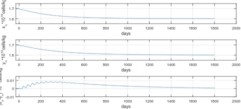
[image:17.595.155.449.590.722.2]According to Theorem 1, when a ∈ (0.2709,0.5) the equilibrium p∗
of CTCS (25) is asymptotically stable and when a ∈ (0,0.2709)∪ (0.5,+∞) the equilibrium p∗ is unstable. Meanwhile, Theorem 2 guarantees that DTCS (26) is asymptotically stable if a∈(ah
1, ah0) and unstable if a∈(0, a1h)∪(ah1,+∞)
for sufficiently small h.
The following Figs.6-9 show the efficiency of control intervals for CTCS and DTCS at same time by choosing initial condition φ(t) = 1.9 cells/kg for t∈[−τ,0]. Fig.6 shows that both continuous-time and discrete-time controllers with h = 5 are invalid for a = 0.26 < a1 (or ah1); and Fig.7 shows that both
two kinds of controllers are efficient for a = 0.285 > a1 (or ah1). On the other hand, choose the initial
days
0 100 200 300 400 500 600 700
xn
*10
10cells/kg
1.2 1.4 1.6 1.8 2
days
0 100 200 300 400 500 600 700
yn
*10
10
cells/kg
1.2 1.4 1.6 1.8 2
continuous-time control
[image:18.595.183.420.210.319.2]discrete-time control
Figure 6: Numerical solutions to Eqs.(25) and (26) witha= 0.26 andh= 5 days.
days
0 200 400 600 800 1000 1200 1400 1600 1800 2000 xn
*10
10
cells/kg
1 1.5 2
days
0 200 400 600 800 1000 1200 1400 1600 1800 2000 yn
*10
10
cells/kg
1 1.5 2
days
0 200 400 600 800 1000 1200 1400 1600 1800 2000 |xn
-yn
|*10
10
cells/kg
[image:18.595.183.421.381.487.2]0 0.05 0.1
Figure 7: Numerical solutions to Eqs.(25) and (26) witha= 0.285 andh= 3 days.
condition φ(t) = 1.7×10¹⁰ cells/kg for t ∈ [−τ,0]. Fig.8 shows that the two controllers are efficient for
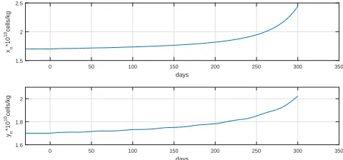
a= 0.49< a0 (or ah0); and Fig.9 shows that both controllers don’t work fora= 0.51> a0 (or ah0).
days
0 200 400 600 800 1000 1200 1400 1600 1800 2000 xn
*10
10
cells/kg
1.6 1.7
days
0 200 400 600 800 1000 1200 1400 1600 1800 2000 yn
*10
10
cells/kg
1.6 1.7
days
0 200 400 600 800 1000 1200 1400 1600 1800 2000 |xn
-y
n
|*10
10
cells/kg
-0.01 0 0.01
[image:18.595.181.421.582.691.2]days
0 50 100 150 200 250 300 350
xn
*10
10
cells/kg
1.5 2 2.5
days
0 50 100 150 200 250 300 350
yn
*10
10cells/kg
[image:19.595.179.419.79.191.2]1.6 1.8 2
Figure 9: Numerical solutions to Eqs.(25) and (26) witha= 0.51 andh= 3 days.
6. Conclusion
In the paper, we have shown that unstable DDE (1) can be asymptotically stabilized by both continuous-time and discrete-continuous-time delay feedback controllers. In fact, our emphasis is on the discrete-continuous-time controller, but in the study process we need the property of characteristic equation for continuous-time model. DTC-S remains asymptotically stable if the CTCDTC-S is so and the sampling period is sufficiently small. Moreover, we also commit ourselves to determining a good bound on sampling period h. Our results can certainly be generalized to cope with more general form of DTCSs. For example,
x′
(t) =f(x(t), x(t−τ)) +a
x
t−τ h
h
−x∗
, t ≥0.
Acknowledgements
This work was supported by the NNSF of 11301115. And the paper was finished during Huan Su visited the University of Strathclyde.
References
[1] G. Chen, J.L. Moiola, H.O. Wang, Bifurcation control: theories, method, and applications, Int. J. Bifurcation Chaos, 10(3)(2000)511-548.
[2] M.A. Kramer, B.A. Lopour, H.E. Kirsch, A.J. Szeri, Bifurcation control of a seizing human cortex, Phys. Rev. E. 73(2006)041928.
[3] K. Engelborghs, V. Lemaire, J. Belair, D. Roose, Numerical bifurcation analysis of delay differential equations arising from physical modeling, J. Math. Biol. 42(2001)361-385.
[4] T. Chen, B. Francis, Optimal Sampled-Date Control Systems, Springer-Verlag, 1995.
[5] K.L. Cooke, J. Wiener, Retard differential equations with piecewise constant delays, Journal of Mathematical Analysis and Applications, 99(1984)265-294.
[6] A.R. Aftabizadeh, J. Wiener, J.M. Xu, Oscillatory and periodic properties of delay differential equations with piecewise constant argument. Proceedings of the American Mathematical Society, 99 (1987)673-679.
[8] X. Mao, Stabilization of continuous-time hybrid stochastic differetnail eqautions by discrete-time feedback control, Automatica. 49 (2013) 3677-3681.
[9] S. You, W. Liu, J. Lu, X. Mao, Q. Qiu, Stabilization of hybrid systems by feedback control based on discrete-time state observations, SIAM J. Control Optim., 53(2015) 905-925.
[10] X. Mao, Almost sure exponential stabilization by discrete-time stochastic feedback control, IEEE Trans. Autom. Control, DOI:10.1109/TAC.2015.2471696.
[11] X. Mao, W. Liu, L. Hu, Q. Luo, J. Lu, Stabilization of hybrid stochastic differential equations by feedback control based on discrete-time state observations,Syst. Control Lett. 73 (2014) 88-95.
[12] M.C. Mackey, L. Glass, Oscillations and chaos in physiological control systems, Science 197 (1977) 287-289.
[13] M. Wazewska-Czyzewska, A. lasota, Mathematical problems of the dynamics of the red blood cells system, Ann. Polish Math. Soc.Ser.III, Appl. Math. 17 (1976) 23-40.
[14] W.S. Gurney, S.P. Blythe, R.M. Nisbet, Nicholson’s blowflies (revised), Nature 287 (1980) 17-21.
[15] J. Wei, Bifurcation analysis in a scalar delay differential equation, Nonlinearity 20 (2007) 2483-2498.
[16] H. Su, X.H. Ding, W.X. Li, Numerical bifurcation control of Mackey-Glass system, Applied Math-ematical Modelling 35 (2011) 2460-3472.
[17] I. Gy¨ori, G. Ladas, Oscillation Theory of Delay Differential Equations with Applications, Oxford University Press, New York, 1991.
[18] A.K. Yuri, Elements of Applied Bifurcation Theory, Spring-Verlag, New York, 1995.
[19] J.K. Hale, Theory of Functional Differential Equations, Springer-Verlag, New York, Heidelberg, Berlin, 1977.


![Figure 4: Numerical solution to Eq.(24) with τ = 30 days and initial condition φ(t) = 1.9 for t ∈ [−τ, 0].](https://thumb-us.123doks.com/thumbv2/123dok_us/1560849.108705/17.595.155.449.590.722/figure-numerical-solution-eq-t-days-initial-condition.webp)