Implementation of a flexible frequency-invariant broadband beamformer based on fourier properties

Implementation of a Flexible Frequency-Invariant

Broadband Beamformer Based on Fourier Properties

Stephan Weiss

∗

, Mark Hadley

†

, and Jon Wilcox

†

∗_{Dept. of EEE, University of Strathclyde, Glasgow G1 1XW, Scotland} †_{Kaon Limited, 5 Wey Court, Guildford, Surrey GU1 4QU, UK}

Abstract—Aperture and operating frequency of a beamformer are generally proportional to its resolution, and inversely pro-portional to its beamwidth. This paper addresses the design and implementation of a beamformer with a frequency-dependent limitation of its aperture such that the frequency-dependence of its resolution is eliminated. Operating across a number of octaves, firstly an octave-invariance design is achieved by means of a nested array structure. Secondly, within each octave, a frequency-dependent aperture control then removes the remain-ing frequency-dependency. By exploitremain-ing Fourier properties and correspondences between coefficient and beamspace, we show that this design is exact, and can accommodate the inclusion of arbitrary shading and different look directions.

I. INTRODUCTION

In broadband sensor applications, the spatial resolution of a beamformer is typically proportional to both the array’s aperture and its operating frequency. For a number of ap-plications, such a microphone arrays, so-called frequency-independent designs have been considered [1]–[21]. These approaches generally create frequency-independence by im-posing the array’s largest beamwidth — defined at the lowest operating frequency — over the entire operating bandwidth by artificially restricting the aperture at higher frequencies.

Most applications of frequency invariant beamforming are in the area of sonar [1] or microphone arrays [2]–[6], where signals extend over several octaves. Unless there are physical restrictions to the array’s size or architecture, such as in the case of hearing aids [4] or for circular arrays [5]–[7], often the frequency-invariant approach has incorporated nested array architectures as discussed in e.g. [1], [8]–[10], which in first instance can be employed to implement an octave-invariant design. Additional processing is then required in order to render a beamformer’s behaviour frequency-invariant within every octave.

The parameters of a frequency-invariant beamformer can be designed via e.g. a direct least squares approach to optimise a desired directivity pattern [4], [6], [7]. In some cases, least squares designs contain additional constraints, such as the minimisation of active sensors via e.g. anl1-norm criterion [5]

or multiple constraints [11]. Other approaches exploit the Fourier correspondence between the coefficient domain and beamspace. This generally involves a design in continuous beamspace based generally on continuous distributed sensors [5], [8], [13]–[17]; the resulting coefficients are then ap-proximated by sampling these continuous functions. In some cases, a two-dimensional array structure can be exploited to

extract temporal information about the signals [12], [18], but in general a tap delay line structure is required to implement such designs. Design methods based in the Fourier equivalence for continuous functions been applied to 1-d [16], [17] and 3-d frequency-in3-depen3-dent arrays 3-designs [8], [13], [14]. For the latter, the design of an approximately rotation-invariant prototype at the lowest frequency, and its translations if the look direction is not towards broadside, forms a particular challenge.

In this paper, we use the nested array approach of [1], [9], [10] and further exploit the Fourier correspondence between the sensor/coefficient domain and beamspace, but instead of constructing an approximation of continuous functions in the discrete domains akin to [8], [13], [14], [16], [17], we directly based our arguments on the discrete Fourier series [22], [23], and show how such a representation that is discrete in beamspace and in the coefficient domain can be accurate. This will enable a very straightforward design and implementation of 1-d frequency-invariant designs.

To motivate this proposed design and implementation, Sec. II reviews the correspondence between coefficient space and beam space, and particularly focuses on the discrete sensor case, and the effect caused by considering only finite samples in beamspace. The octave-invariant approach and general design of invariance within octaves is outlined in Sec. III, followed by considerations regarding arbitrary win-dows, such as Dirichlet kernels, Hamming or Taylor winwin-dows, and arbitrary look directions in Secs. IV and V. Comment on both the coefficient design and the overall implementation of the beamformer using an overlap-add approach are detailed in Sec. VI. Examples are provided throughout the paper, and conclusions are drawn in Sec. VII.

II. BEAMSPACETRANSFORM

For a set of beamformer coefficients w[m] applied to a linear uniform array of M sensors, where m ∈ Z is the discrete sensor index, the transformation to beamspace with dependency on a continuousΨ∈Ris performed by a Fourier transform,

W(ejΨ) =

∞ X

m=−∞

w[m]e−jΨm_.

Becausew[m]is discrete,W(ejΨ_{)is periodic w.r.t.Ψ = 2πk,}

k∈Z. The inverse transform

w[m] = 1 2π

π

Z

−π

W(ejΨ_)ejΨm_{dΨ. (2)}

exploits the periodicity by evaluating only over the interval

Ψ∈(−π;π). A transform pair according to (1) and (2) will be abbreviated by w[m]◦—•W(ejΨ_{)in the following.}

We now consider a finite aperture afforded by M sensors such that w[m]6= 0∀ |m|< M/2 withM odd. Discretising the beamspace toMdiscrete equidistant valuesΨk= 2πk/M, k∈Z, on the interval(−π;π)we have

W(ejΨk) =

∞ X

m=−∞

w[m]e−jΨkm_,

k=−M−1

2 . . .

M−1

2 . (3)

The function corresponding to (3) in the coefficient domain,

˜

w[m], is a periodised version of w[m] w.r.t. kM,k ∈ Z. If however only a fundamental period of w˜[m] is retained, the discretisation of Ψis without consequences:

w[m] = 1

M

(M_X−1)/2

k=−(M−1)/2

W(ejΨk)ejΨkm,

m=−M −1

2 . . .

M −1

2 . (4)

Therefore for a discrete w[m] with finite aperture M, the concatenation of the discretised versions (3) and (4) is an exact alternative to calculating the continuous beamspace transforms in (1) and (2).

III. FREQUENCY-INVARIANTBEAMFORMERDESIGN

This section explains the general approach by Van Trees and Bell [9] to achieve constant resolution across all frequencies. The analysis will form the basis of developments in the subsequent sections.

Resolution is proportional to aperture and frequency. Sec. III-A produces an octave-invariant resolution by means of a nested array, where a wider aperture compensates the frequency-related loss in resolution in lower bands. Sec. III-B creates frequency-invariance within one octave by algorithmi-cally reducing the aperture inversely proportional to frequency.

A. Octave-Invariant Approach Using Nested Arrays

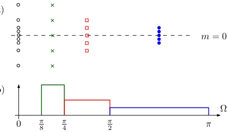
To achieve an octave-invariant design, a nested array as detailed in [1], [9], [10] is employed. At the highest octave, the array is operated with a given aperture. For the next-lower octave, this aperture is doubled; this scheme is continued over the number of octaves of which the bandwidth comprises. As the frequency band of each octave decreases, thus the aperture is doubled in terms of distance so that it is equalised in terms of wavelengths. Fig. 1 provides an example for three octaves, whereby within each octave an array of M = 5 sensors is utilised. The aperture is increased by scaling the array, e.g. by

a)

Ω

π π

2

0 π

4

π

8

b)

[image:2.612.316.539.52.181.2]

m= 0

Fig. 1. (a) Nested sensor array (left) and the assignment of sensors to three different linear uniform subarrays (right). The centre element in each subarray is the reference sensor with indexm= 0; (b) octaves in which the subarrays are processed.

doubling the separation distance between sensors with every lowering by a octave.

For a linear array, such a nested approach can be constructed for an arbitrary number of sensorsM. However, it is easy to see that a particularly efficient re-use of sensor is possible if each band comprises ofM = 4k+1,k∈Z, array elements. In this fashion, the elements at the end of the array for a particular octave can always be acquire signals for the next-lower octave as well.

B. Frequency-Invariance within one Octave

The idea to achieve frequency-invariance is to restrict the aperture at every frequency such that it matches the lowest resolution within the array. We first design coefficients for the highest octave, covering theΩ∈(π

2, π). The lowest resolution

is atΩ = π

2, where the coefficient set should satisfy a Dirichlet

kernel [22],

pM[m]◦—•

sinMΨ₂

sinΨ 2

=PM(ejΨ). (5)

At the upper end of the frequency range forΩ =π, the resolu-tion should be reduced to an aperture ofM/2. Directly scaling pM[m]results in fractional values forM and implementation

challenges akin to those known for fractional delay filters [24]. Instead, scaling will be performed in beamspace, resulting in a sinc-interpolated scaled coefficient domain quantity.

The Fourier transform’s scaling property

|a|x(at)◦—•X(jΩ/a) only applies if x(t) depends on a continuous variablet, but can be made to work with a trick. First, we produce an aperiodic function containing a fraction

1/aof the original period in beamspace,

˜

PM(jψ) =PM(ejψ), |ψ|< π

a (6)

This coefficient-domain function equivalent to (6) is now dependent on continuous space. Thus, it can be scaled, and thereafter is periodised again, s.t.

¯

PM(a, ejΨ) = ˜PM(jaψ), Ψ =aψ+ 2πk, k∈Z. (7)

As a result of scaling and periodisation, P¯M(a, ejΨ) may

0.25 0.3

0.35 0.4

0.45 0.5

−10 −5

0 5 10

0 0.02 0.04 0.06 0.08 0.1

¯

pM

,

2

Ω

/

π

[

m

]

[image:3.612.49.301.54.198.2]

Ω 2π angleϑ/[◦_]

Fig. 2. Coefficient space windowp¯M,2Ω/π[m]over one octave, depending on normalised angular frequencyΩand coefficient indexm.

¯

PM(a, ejΨ) at ±π; however, no other approximation errors

are incurred.

Because of the periodicity of P¯M(a, ejΨ), the coefficient

domain functionp¯M,a[m]•—◦P¯M(a, ejΨ)is still discrete. If

Ψ is discretised withΨk = 2πk/M,k∈Z, then p¯M,a[m] is

periodised w.r.t.M. Therefore, analogous to the arguments in Sec. II, we can employ the inverse discrete Fourier transform from beamspace, and only retain the fundamental period of

¯

pM,a[m], |m| ≤(M −1)/2 to obtain the desired coefficient

domain function.

A shortcut is to sample PM(ejψ)in (6) directly instead of

¯

PM(a, ejΨ)in (7). Thus

¯

pM,a[m]◦—•PM(ejψk) (8)

forψk= 2_aMπk with|k|,|m| ≤(M−1)/2.

Based on the above analysis, the coefficient domain win-dow is adjusted in a frequency dependent fashion s.t. at a frequency π₂ ≤ Ω < π we employ a window p¯M,a[m] with a = 2Ω/π, or short p¯M,2Ω/π[m], which is obtained by an

inverse discrete Fourier transform according to (8). For an example with M = 21, the resulting frequency-dependent coefficient domain window p¯M,2Ω/π[m] is shown in Fig. 2,

with the narrowing of the window with frequency clearly evident. The directivity pattern for this beamformer is depicted in Fig. 3, demonstrating frequency invariance over one octave.

IV. ARBITRARYWINDOWING

The window design in Sec. III-B is restricted to the rect-angular window of (5). This section explores the inclusion of arbitrary window shapes into the frequency-invariant design.

To obtain an arbitrary window shape wM[m], whereM is

the total array aperture and mthe sensor index,

wM[m] =pM[m]·vM[m] (9)

multiplies the rectangular windowpM[m]with a taper function v[m], such as a von Hann, Hamming or Taylor window. In the beamspace domain, the equivalent to (9) is a convolution of

0.25 0.3

0.35 0.4

0.45 0.5

−80 −60 −40 −20 0 20 40 60 80 −60 −40 −20 0

2

0

lo

g1

0

|

A

(

ϑ

,e

j

Ω)

|

/

[d

B

]

Ω 2π angleϑ/[◦_]

Fig. 3. Directivity pattern for the beamformer in Fig. 2.

the Fourier transforms ofpM[m] andvM[m],

WM(ejΨ) = π

Z

−π

PM(ej(Ψ−Φ))VM(ejΦ)dΦ. (10)

Writing the windowVm(ejΨ)in its Fourier expansion, VM(ejΨ) =

K

X

k=−K vk

X

l∈Z

δ(Ψ−2πl−2πk

M ) (11) can be efficient, as the integral in (10) only extracts a single term of the impulse train in (11), and since in general K is small. For example, von Hann and Hamming windows are exact withK= 1, and a Taylor window can be approximated to already high accuracy withK= 2. This leads to simplifying (10) to

WM(ejΨ) = K

X

k=−K

vkPM(ej(Ψ−

2πk

M )) ₍₁₂₎

Inserting WM(ejΨ) instead of PM(ejψ) into (6), a scaled

version of a tapered window can be constructed analogously to the derivation in Sec. III-B.

More directly, a discretised scaled version

¯

WM,a(ejΨk) = K

X

k=−K

vkPM(ej(Ψk/a−

2πk

M)) ₍₁₃₎

can be calculated with Ψk = 2πk/M, Z ∋ |k| ≤ (M −

1)/2, such that a suitably scaled coefficient domain window wM,a[m]is obtained by an inverse DFT of (13). Analogously

to considerations in Sec. III-B, the coefficient domain function is exact despite the discretisation of (13) in beamspace.

An example for the earlier array withM = 21but applying a Taylor window is shown in Fig. 4 for the highest octave band. The directivity pattern for this array is provided in Fig. 5.

V. ARBITRARYLOOKDIRECTION

Given that an array response in beamspace,W¯(ejΨ_{)is of}

0.25 0.3

0.35 0.4

0.45 0.5

−10 −5

0 5 10

0 0.05 0.1 0.15

¯

wM

,

2

Ω

/

π

[

m

]

[image:4.612.306.560.54.195.2]

Ω 2π angleϑ/[◦_]

Fig. 4. Coefficient space windoww¯M,2Ω/π[m]with a frequency-invariant Taylor design over one octave, depending on normalised angular frequency Ωand coefficient indexm.

0.25 0.3

0.35 0.4

0.45 0.5

−80 −60 −40 −20 0 20 40 60 80 −60 −40 −20 0

2

0

lo

g1

0

|

A

(

ϑ

,e

j

Ω)

|

/

[d

B

]

Ω 2π angleϑ/[◦_]

Fig. 5. Directivity pattern for the beamformer in Fig. 4.

angle of arrival measured against broadside, it is possible to alter an array to look towards an angleϑ0, i.e.Ψ0= 2πsinϑ0,

by altering the response to

Wϑ0(e

jΨ_{) = ¯W(e}j(Ψ−Ψ0)

). (14) To generalise the previous design to a different look direction, (13) simply becomes

¯

WM,a,ϑ0(e

jΨk_{) =}

K

X

k=−K

vkPM(ej((Ψk−Ψ0)/a−

2πk

M)), ₍₁₅₎

from which the coefficients can be obtained by an inverse discrete Fourier transform.

Extending the earlier example of a Taylor window design for an array of M = 21 elements per octave to a look direction ϑ0 = 30◦ yields coefficients with the same magnitude but

different phase to those shown in Fig. 4. This phase shifts leads to the approximately frequency-invariant directivity pattern in Fig. 6, which exhibits the desired look direction.

VI. IMPLEMENTATION

A. Independent Frequency Bin Processor

If the beamformer is to measure received power versus angle of arrival and frequency, a simple independent frequency bin (IFB) processor can be employed. The sensor signals are

0.25 0.3

0.35 0.4

0.45 0.5

−80 −60 −40 −20 0 20 40 60 80 −60 −40 −20 0

2

0

lo

g1

0

|

A

(

ϑ

,e

j

Ω)

|

/

[d

B

]

[image:4.612.50.295.54.196.2]

Ω 2π angleϑ/[◦_]

Fig. 6. Directivity pattern for a beamformer with look directionϑ0= 30◦.

0.1 0.2

0.3 0.4

0.5

−80 −60 −40 −20 0 20 40 60 80 −60 −40 −20 0

angleϑ/[◦_]

2

0

lo

g1

0

|

A

(

ϑ

,e

j

Ω)

|

/

[d

B

]

Ω 2π

Fig. 7. Overlap-add implementation of a nested array frequency invariant beamformer operating over 4 octaves,Ω∈(2π

32; 2π

2 ), with a Taylor window

design and look directionϑ0= 30◦.

decomposed by sufficient large DFT/FFT, and each frequency bin is processed independently, thus neglecting coherence across the spectrum. An IFB processor is straightforward and consist of drawing specific frequency bins from specific sensors according to the nested array structure outlined in Fig. 1. The directivity pattern of such a beamformer is the same as those shown in Figs. 3, 5 and 6, but extends over the number of octaves included in the nested array structure as shown in Fig. 7.

B. Overlap-Add Implementation

If the beamformer is to act as a spatio-temporal filter with a time-domain signal as output, then the frequency-dependent design of the beamforming coefficients in Secs. III – V requires a frequency-domain implementation of the beam-former, such as overlap-add/overlap-save techniques [25]. An overlap-add approach is used here, which requires time domain filters that are zero-padded. This can be achieved by oversam-pling the frequency domain representation of the beamformer weights by a factor of two, eliminating a periodic repetition in the time domain, and transforming back to the frequency domain again, thus interpolating the initially oversampled representation.

[image:4.612.308.563.231.373.2] [image:4.612.49.295.245.384.2]

will exhibit Gibbs phenomena [22] at the lower and upper ends of the band of interest. The directivity pattern in Fig. 7 is measured from an overlap-add implementation that has been excited by broadband steering vectors [26], [27] from different angles of arrival, and shows such Gibbs phenomena particularly at the lower end of the operating spectrum at around Ω = π

8, but without wider impact on the accuracy

and frequency invariance of the array’s response.

VII. CONCLUSION

This paper has presented a simple 1-d frequency-invariant beamformer design that can accommodate bandwidths stretch-ing across several octaves. This is accomplished by a combi-nation of an nested array, which creates an octave-invariant design, and a design approach that within every octave re-strictes the aperture in a frequency-dependent fashion such that the overall directivity patterns is constant across the desired bandwidth. The latter part exploits exact properties of the Fourier series, i.e. when applied to discrete sensors and to discrete points in beamspace.

The design can accommodate arbitrary window functions such as a Dirichlet kernel, von Hann, Hamming or Taylor windows, or others. Also, the direction of the beamformer can be selected off-broadside. The calculation of the beamformer coefficients, the window implementation, off-broadside look diections, as well as the overall beamformer implementation using overlap-add techniques are sufficiently simple to be applicable to arbitrarily large arrays. By examples, we have demonstrated the various aspects, accuracy and simplicity of the beamformer design.

ACKNOWLEDGEMENT

This work was supported in parts by the Engineering and Physical Sciences Research Council (EPSRC) Grant number EP/K014307/1 and the MOD University Defence Research Collaboration in Signal Processing.

REFERENCES

[1] R. Smith. Constant beamwidth receiving arrays for broad band sonar systems.Acoustica, 23:21–26, 1970.

[2] H. Barfuss, C. Huemmer, G. Lamani, A. Schwarz, and W. Kellermann. HRFT-based robust least-squares frequency-invariant beamforming. In

2015 IEEE Workshop on Applications of Signal Processing to Audio and Acoustics (WASPAA), pages 1–5, Oct 2015.

[3] O. Rosen, I. Cohen, and D. Malah. FIR-based symmetrical acoustic beamformer with a constant beamwidth. Signal Processing, 130:365 – 376, 2017.

[4] M. Crocco and A. Trucco. Design of robust superdirective arrays with a tunable tradeoff between directivity and frequency-invariance. IEEE Transactions on Signal Processing, 59(5):2169–2181, May 2011. [5] S. C. Chan and H. H. Chen. Uniform concentric circular arrays with

frequency-invariant characteristics mdash;theory, design, adaptive beam-forming and doa estimation. IEEE Transactions on Signal Processing, 55(1):165–177, Jan 2007.

[6] G. Huang, J. Benesty, and J. Chen. On the design of frequency-invariant beampatterns with uniform circular microphone arrays. IEEE/ACM Transactions on Audio, Speech, and Language Processing, 25(5):1140– 1153, May 2017.

[7] Y. Wang, Y. Yang, Z. He, Y. Ma, and B. Li. Robust superdirective frequency-invariant beamforming for circular sensor arrays.IEEE Signal Processing Letters, PP(99):1–1, 2017.

[8] W. Liu and S. Weiss. Wideband Beamforming — Concepts and

Techniques. Wiley, 2010.

[9] H. L. Van Trees. Detection, Estimation and Modulation Theory: Optimum Array Processing. Wiley, New York, 2002.

[10] S. Weiss, R. W. Stewart, and W. Liu. A Broadband Adaptive Beamform-ing Structure with Scaled Aperture. InThirty-Sixth Asilomar Conference on Signals, Systems and Computers, volume 2, pages 1298–1302, Pacific Grove, CA, November 3–6 2002.

[11] Y. Liu, L. Zhang, L. Ye, Z. Nie, and Q. H. Liu. Synthesis of sparse arrays with frequency-invariant-focused beam patterns under accurate sidelobe control by iterative second-order cone programming.IEEE Transactions on Antennas and Propagation, 63(12):5826–5832, Dec 2015. [12] W. Liu, D. C. McLernon, and M. Ghogho. Design of frequency invariant

beamformer without temporal filtering. IEEE Transactions on Signal Processing, 57(2):798–802, Feb 2009.

[13] W. Liu and S. Weiss. Design of frequency invariant beamformers for broadband arrays. IEEE Transactions on Signal Processing, 56(2):855– 860, Feb. 2008.

[14] W. Liu, S. Weiss, J. McWhirter, and I. Proulder. Frequency invariant beamforming for two-dimensional and three-dimensional arrays. Signal Processing, 87(11):2535–2543, November 2007.

[15] J. S. Marciano and T. B. Vu. Reduced complexity beam space broadband frequency invariant beamforming. Electronics Letters, 36(7):682–683, Mar 2000.

[16] D. B. Ward, R. A. Kennedy, and C. Williamson, R. Theory and design of broadband sensor arrays with frequency invariant far-field beam patterns.

Journal of the Acoustic Society of America, 97(2):1023–1034, 1995. [17] D. B. Ward, R. A. Kennedy, and C. Williamson, R. FIR filter design

for frequency invariant beamformers. IEEE Signal Processing Letters, 3:69–71, 1996.

[18] P. Pal and P. P. Vaidyanathan. Efficient frequency invariant beamforming using virtual arrays. In2010 Conference Record of the Forty Fourth Asilomar Conference on Signals, Systems and Computers, pages 1097– 1101, Nov 2010.

[19] F. Traverso, M. Crocco, and A. Trucco. Design of frequency-invariant robust beam patterns by the oversteering of end-fire arrays. Signal Processing, 99:129 – 135, 2014.

[20] Y. Zhao and W. Liu. Robust fixed frequency invariant beamformer design subject to norm-bounded errors.IEEE Signal Processing Letters, 20(2):169–172, Feb 2013.

[21] L. Parra. Steerable frequency-invariant beamforming for arbitrary arrays.

Journal of the Acoustical Society of America, 119:3839–3847, June 2006.

[22] V. Pohl and H. Boche. Advanced topics in system and signal theory. Springer, Heidelberg, 2009.

[23] E. M. Stein and R. Shakarchi. Fourier analysis: an introduction. Princeton University Press, 2003.

[24] T. I. Laakso, V. V¨alim¨aki, M. Karjalainen, and U. K. Laine. Splitting the unit delay.IEEE Signal Processing Magazine, 13(1):30–60, January 1996.

[25] R. E. Crochiere and L. R. Rabiner.Multirate digital signal processing. Prentice Hall, Englewood Cliffs, NJ, 1983.

[26] J. Selva. An efficient structure for the design of variable fractional delay filters based on the windowing method. IEEE Transactions on Signal Processing, 56(8):3770–3775, August 2008.