A Two-loop Optimization Strategy for Multi-objective Optimal Experimental
Design
Hui Yu*, Hong Yue*, Peter Halling**
* Department of Electronic and Electrical Engineering,University of Strathclyde, Glasgow G1 1XW, UK
** Department of Pure and Applied Chemistry,University of Strathclyde, Glasgow G1 1XL, UK (e-mail: [email protected], [email protected], [email protected])
Abstract: A newstrategy of optimal experimental design (OED) is proposed for a kinetically controlled synthesis system by considering both observation design and input design. The observation design that combines sampling scheduling and measurement set selection is treated as a single optimization problem arranged in the inner loop, while the optimization of input intensity is calculated in the outer loop. This multi-objective dynamic optimization problem is solved via the integration of particle swarm algorithm (for the outer loop) and the interior-point method (for the inner loop). Numerical studies demonstrate the efficiency of this optimization strategy and show the effectiveness of this integrated OED in reducing parameter estimation uncertainties. In addition, process optimization of the case study enzyme reaction system is investigated with the aim to obtain maximum production rate by taking into account of the experimental cost.
Keywords: multi-objective optimal experimental design (OED), process optimization, observation strategy, input design, parameter estimation, enzyme reaction system.
1. INTRODUCTION
Mathematical models are widely used in process systems engineering especially when using modern techniques (Peleg, et al., 2002). Model development includes determining suitable model structure and estimation of unknown model
parameters (Franceschini and Macchietto, 2008).
Biochemical processes are normally highly nonlinear and
contain complex dynamic behaviours. Intuitive
experimentation for these systems may produce data lacking effective modelling information, which therefore affects the parameter estimation quality. Collecting rich data for biochemical systems through experimentation is also cost intensive and time consuming. Therefore, designing experiment to generate efficient data is crucial for modelling of complex systems. Incorporating optimal experimental design (OED) into parameter estimation procedure has a good potential to improve estimation quality for high-dimension systems with sparse and noisy data for model development. Here OED refers to devising experiments to obtain the most informative data so that the model parameters can be estimated from those measurement data with the best statistical quality (Faller, et al., 2003). A number of methods have been developed and successfully applied in modelling of biological and biochemical systems (Atkinson, et al., 2014; Baltes, et al., 1994; Liepe, et al., 2013; Walter and Pronzato, 1990; Yu, et al., 2015).
Experimental design for parameter estimation may need to handle the choice of input conditions, sampling strategy, measurement state subset and other factors associated with either input signals or measurement data. An OED problem can be formulated as dynamic optimization problem with
respect to the design factors of interest, where the major objective is to maximise the data information through a measure of certain scalar function of Fisher information matrix (FIM). Since biochemical systems are often described by nonlinear and stiff differential equations, the OED problem is normally non-convex, so it is hard to find the optimal solution. Various methods have been proposed to solve this optimization problem, among them a popular method, called the control vector parameterization (CVP) method, which discretizes the control variables and transfer the OED problem into a nonlinear programming (NLP) problem (Balsa-Canto, et al., 2008; Bauer, et al., 1999; Bauer, et al., 2000). However, by considering input factors and observation factors together, the degrees of freedom in OED are greatly increased, which makes it extremely difficult to find the optimal solution. Traditional methods such as sequential quadratic programming may lead to local minimal solution only (Banga, et al., 2002). Stochastic algorithms aiming for a global solution are computationally expensive. It is therefore necessary to develop an efficient strategy for a complex OED that includes both input and observation design. This is the main motivation of this work.
the inner loop for observation design and the outer loop for input design.
Process optimization is also a challenging task for the case study enzymatic reaction system, where the product of interest is not the thermodynamically most favourable one among all reactants. A successful operation should aim to achieve maximum product quantity with the consideration of production cost. Preliminary investigation of this process optimisation task is attempted in this work.
The rest of the paper is organized as follows. In Section 2, preliminaries on parameter estimation and its relation to Fisher information matrix are briefly introduced. In Section 3, the multi-objective OED problem is formulated and the double-loop solution strategy is presented. The proposed OED algorithm is applied to an enzyme kinetically controlled synthesis system and the process optimization is also discussed in Section 4. Finally, conclusions and discussions are given in Section 5.
2. PRELIMINARIES
Consider a general nonlinear model for a biochemical system described in the form of ordinary differential equations:
0 0f , , ,t t
X X θ X X (1)
h , ,t
Y X θ ξ (2)
where X[ ,x x1 2, ,xn]T n denotes the vector of n state variables with initial condition X0; θ[ ,k k1 2, kp]T p
is the vector of p model parameters; f
is a set of state transition functions which are assumed to be continuous andfirst-order derivative; Y m is the measurement output
vector with m m
n
measurable variables, and h
is the measurement function, normally used for selecting whichvariables to be measured. ξ is the measurement noise which
is assumed to be independently and identically distributed (i.i.d.), zero-mean Gaussian noise. In practice, some model parameters are known and need to be estimated by comparing model prediction with experimental data. The most prevalent method for parameter estimation is the (weighted) least-square estimation, where the problem is formulated as:
22 1 1
ˆ argmin
1 1 ˆ
arg min ,
2 m N
i l i l i l i
J
y t y t
θ
θ
θ θ
θ (3)
where y ti
l and yˆi
θ,tl are measured values and modelprediction of the i-th state variable, respectively, at sampling times tl (l1, 2,3, ,N), N is the total number of sampling
data in the time dimension. 2
i
denotes the measurement
error variance of the i-th state variable which is used to compensate measurement uncertainties.
Once parameter estimation is conducted, it is necessary to assess the adequacy of the model and parameter significance
by evaluating the output residuals through statistical tests. A lack-of-fit test is normally applied to evaluate whether the structured model can explain the experimental data satisfactorily. Regarding parameter estimation, the student t-test and the method based on joint confidence regions between parameters are two widely used methods to evaluate the estimation quality (Franceschini and Macchietto, 2008). The latter (Motulsky and Christopoulos, 2004) is used in this work. The confidence region can be determined based on the cost function in (3):
1
, ˆ
:J 1 p Fp N p J N p
θ θ θ (4)
where 1
,
p N p
F is the upper (0 1)-critical level of the
F distribution with p and (Np) degrees of freedom,
(0 1)
is a positive real number. However, for a
nonlinear model, J
θ is not a quadratic function withrespect to θ, and a linearization approximation is made by the
second-order Taylor series expansion around the estimated
parameters θˆ . The confidence region can then be
approximated as:
T
1 1
,
ˆ ˆ ˆ
p N p p F
θ θ V θ θ θ (5)
where
ˆ 1 2ˆ ˆ
2 J , JT
N p
θ
V H θ H θ
θ θ (6)
Here V is the parameter estimation error covariance matrix which is used as the cornerstone to measure parameter estimation uncertainty. J
θˆ
Np
is an approximation of residual variance. H is the Hessian matrix. The confidence interval of a single parameter ki can be determined byi tN p ii
V (7)
where tN p is the student distribution with (1) confidence
level and (Np) degrees of freedom.
The FIM is defined by T 1
FIM S Q S, where S X θ is
the local parametric sensitivity matrix, and Q is the
measurement error covariance matrix. It can be seen that the FIM is approximately equal to the inverse of the parameter estimation error covariance matrix, thus can be used to
approximate V. It provides the lower bound of the parameter
estimation errors based on the Cramer-Rao inequality (Ljung, 1987). Many OED techniques are therefore developed based on FIM.
3. MULTI-OBJECTIVE OPTIMAL EXPERIMENTAL DESIGN
Denote the design factors which characterize the experiment into a vector ζ, the FIM can be written as:
,
, T 1
,FIM θ ζ S θ ζ Q S θ ζ (8) The OED problem can be cast as the minimization of a proper measure of FIM, i.e.
*
arg max ,
ζ Ω
ζ FIM θ ζ (9)
where Ω is the admissible space of design factors,
represents a function to scalarise the FIM. The most commonly used design criteria are A-optimal, D-optimal, E-optimal, and modified E-optimal design (Hosten, 1974; Ljung, 1987).3.2 Multi-task Observation Design
In this work, observation design consists of two aspects: (a) the selection of measurement set; and (b) the choice of sampling time strategy. In measurement set design, the most informative measurable state variables will be determined for parameter estimation. This problem can be represented as follows (Brown, et al., 2008; He, et al., 2010):
1 1 1 2 T 1 T mins.t. 0,1 ,
n n n
i i i i i sel x x n
S S1 λ
(10)
where i is an integer weight with values of 0 or 1, relating to the i-th state variable, nsel is the total number of selected measurement state variables. The variance terms of measurement noise are considered to be the same and are constant for all the noise channels, therefore has no effect to the optimization design.
The optimal sampling design is to determine the best sampling (time) schedule for the measurable variables that will provide the most informative experimental data for parameter estimation. For a continuous-time dynamic system, choosing sampling points in the time horizon is an infinite dimensional non-convex dynamic optimization problem, which is hard to solve. Therefore, the sampling time design for most biochemical systems is dealt with as a discrete optimization problem where the available measurement points are defined in priori (Kutalik, et al., 2004):
1 2 1 2 T * 2 1 T arg min. . 0,1
N N N
i i i i
i sp
t t t
t t s t N
ω Ω ζζ S S
1 ω
(11)
where ω
1 N
T is the weighting vector for allavailable measurement points. Nsp is the total number of
sampling points to be selected.
When the measurement set selection and sampling design is integrated together, it provides a wide option that both measurement set and sampling time are free to choose within the design domain. Each state variable at each available sampling point is given a small weighting. The observation design problem can be defined in a similar form to (11), and the only difference is that the number of the integrated
weighting factors is extended to n N . This integer
optimization problem can then be transferred into a continuous optimization problem by relaxing the weightings to a continuous value between [0, 1] shown as:
1 2 1 2 T * 2 1 T arg mins.t. 0, 1 , .
N n N n N n
i i i i
i sp
t t t
t t N
ω Ω ζζ S S
1 ω
(12)
At each sampling time point the FIM for each measurable state variable is a positive definite matrix. Therefore, the continuous optimization problem can be converted into a convex optimization problem by using different scalar design criteria. In this work the D-optimal criterion is used and the design problem can be formulated as a finite-dimension constrained linear optimization problem which can be solved by the interior-point method (Boyd and Vandenberghe, 2004).
3.3 Integration of Observation Design and Input Design
To consider the overall experimental operations, both input and observation strategies should be handled in an integrated framework. Since the change of input conditions will inevitably affect the system dynamics, the input design problem is formulated as a complex non-convex optimization problem. On the other hand, the observation design problem can be reduced to a convex optimization problem as mentioned in Section 3.2. As such, there is no simple solution for this multi-objective optimization problem.
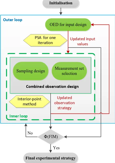
In this work, we propose to solve this integrated design problem with a two-loop sequential numerical procedure as shown in Fig. 1. Within the context of biochemical systems, here the input design refers to the calculation of initial concentrations of reactants. The input signal design is arranged in the outer loop, and the observation design is put in the inner loop. In this structure, the input signals are firstly determined by one iteration update of particle swarm algorithm, based on which the observation design problem is solved in the inner loop with the interior-point method. The designed observation strategy is then used in the next iteration of outer-loop input signal design. This process will continue until the optimal solution is obtained.
conditions, the outer-loop design with stochastic searching largely increases the chance of finding a global solution. This is a clear advantage over the traditional local numerical algorithm, e.g. sequential quadratic programming (SQP) method. For a complex design problem including both input signal design and observation design, it is also computationally more efficient to put the observation design within the inner loop since this is a convex optimization problem that is relatively easy to solve.
OED for input design
Final experimental strategy
Yes No
Initialisation
Interior-point method
PSA for one iteration
Outer loop
Inner loop
(FIM)
Updated observation
strategy
Updated input values
Sampling design Measurement set selection
[image:4.595.57.282.188.508.2]Combined observation design
Fig. 1 Numerical strategy for multi-objective OED problem
4. CASE STUDY FOR AN ENZYME REACTION SYSTEM
4.1 Sensitivity Analysis and Identifiability Analysis
An enzyme kinetically controlled synthesis process is considered in this work. The detailed model description, the nominal values of all parameters and initial conditions, and local sensitivity analysis (LSA) can be found in (Yue, et al., 2013). In this enzyme process, the experimental length is set to be 100 minutes and sampling takes place in every minute. Previous work has shown that the three most sensitive
parameters are k W5 , k3 and k3 from the measure of
integrated local sensitivities. However, this local sensitivity analysis does not consider correlations between parameters. In biochemical systems, correlations between kinetic parameters are often seen in reversible reactions. The
parameter correlation between ki and kj can be determined from FIM as:
cov i, j
ij
ii jj k k R
FIM FIM
(13)
The correlation matrix is composed of Rij, in which except for the diagonal elements, any entries with values close to
1
suggests a strong correlation between the two involved
parameters. This will cause problems in parameter identifiability. Fig. 2 describes the parameter pair correlation for the enzyme reaction model, where
k k1, 1
,
k3, k3
,
k5W,k5
,
k5W,k6
,
k5,k6
are seem to be highlycorrelated. The orthogonalized sensitivity methods, which include forward selection and backward elimination, are used in this work for the selection of key parameters (Yao, et al., 2003). The detailed ranking results are shown in Table 1. It is worth noting that the ranking difference between LSA and the orthogonalized sensitivity methods are very obvious. k3
and k3 are the two most important parameters via LSA
[image:4.595.321.524.431.591.2]ranking. However, when considering the high correlation level between these two parameters, it is found that they cannot be identified simultaneously (see Fig. 2). Therefore, the orthogonalization based methods provide more reliable results in parameter ranking. From the parameter identifiability analysis, k3, k W5 and k2 are found to be the three most important and identifiable parameters.
Fig. 2 Visualization of parameter pair correlations
Table 1 Comparison of different parameter importance ranking result
Parameter ranking methods
Parameter importance rankings
LSA k-3 k3 k5W k2 k4 k-4 k-2 k-5 k6
k1 k-1
Orthogonal forward selection
k-3 k5W k2 k1 k4 k3 k-2 k6 k-4
k-1 k-5
Orthogonal backward elimination
k-3 k5W k2 k4 k3 k-2 k6 k1 k-5
4.2 Design of Observation Strategy
[image:5.595.304.554.210.588.2]Once k3,k W5 and k2 have been determined as the most important parameters, the OED for the estimation of these key parameters is applied in order to find the best observation schedule. Assuming that one hundred evenly space data points for each measurable state variable are available sampling points, the objective is to find 20 measurement data points that will lead to the most information. The D-optimal criterion is used to measure the data information and the design result is shown in Table 2. It can be seen that by using the OED techniques, the determinant of FIM increases almost three orders of magnitude which means that on average the uncertainty of each parameter is decreased nearly 30%, which is a significant improvement for the increase of parameter precision. Furthermore, we can see that the design result suggests the measurement of S to be taken from 10 to 15 minutes and from 53 to 59 minutes, and the measurement of Q to be taken from 71 to 77 minutes. These two state variables are determined as the most valuable states and the measurement of them can lead to the most informative experimental data. Note that the observation design only manipulates the measurement strategy while the system dynamic is not changed. This also indicates that the model-based OED is very necessary in the improvement of parameter estimation precision.
Table 2 Measurement strategy from observation design
Measurable state variables
Non-designed sampling (unit: min)
Designed sampling (unit: min)
S 25, 50, 75, 100 10-15, 53-59
P 25, 50, 75, 100 /
N 25, 50, 75, 100 /
Q 25, 50, 75, 100 71-77
R 25, 50, 75, 100 /
Det(FIM) 2.986e-8 2.428e-5
4.3 OED for All Design Factors
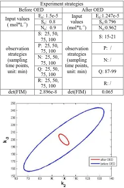
The observation design has already shown very significant improvement in reducing parameter estimation uncertainty. Now we consider the OED for all design factors including observation strategy and input signals. The D-optimal design result is shown in Table 3. It can be seen that S and Q are still determined as the most valuable state variables which is consistent with the observation design results. However, it is suggested that measurement of S should only be taken in the early reaction, while in the middle of reaction S does not need to be measured. This is different from the observation design result. It can be seen that after OED the increase of the objective value is up to six orders of magnitude, which is
obviously better than the observation design. Fig. 3 shows the confidence intervals of k2 and k3 with different experiment
strategies. It is found that that the uncertainty of k3 is only
around 5% after experimental design, while experimentation with nominal conditions (before OED) may results in the
uncertainty of k3 to be more than 20%, similar improvement
for k2 with uncertainty from 34% (before OED) to 5% (after
OED).
Table 3 Comparison of experimental conditions before OED and after OED
Experiment strategies
Before OED After OED
Input values ( mol*L-1)
E0: 1.5e-5 Input
values (mol*L-1)
E0:1.247e-5
S0: 0.8 S0:0.796
N0: 0.9 N0:0.962
observation strategies (sampling time points,
unit: min)
S: 25, 50, 75, 100
observation strategies (sampling time points,
unit: min)
S: 15-21
P: 25, 50,
75, 100 P: /
N: 25, 50,
75, 100 N: /
Q: 25, 50,
75, 100 Q: 87-99
R: 25, 50,
75, 100 R: /
det(FIM) 2.896e-8 det(FIM) 0.065
Fig. 3 Comparison of CI ellipsoids for [k2, k-3] with different
experiment strategies
4.4 Process Optimization
[image:5.595.43.292.434.599.2]input variables and process time that will give the best possible outcome as defined by a certain objective function. Therefore, the user is more concerned with model behaviour only in that small region around the point where the optimal condition can be achieved. To this point, model identification should be integrated with process optimization so that the model will be more accurate in that region of state space of interest.
Now we look at the process optimization of this enzyme kinetic model to investigate how the input values will affect the process behaviour. It is also primary work for further integration of process optimization and parameter estimation. In this case there are three input values which are E0, N0 and
S0. The aim is to optimize these three input values in order to
obtain the most possible outcome of Q with the consideration of the budget. Therefore, the objective can be defined as:
0
0 0
arg max(aQ bS cE )
test
test T
Obj
X Ω
(14)
where X0 is the vector of input state variables. The
coefficients a, b and c represents the unit price of Qtest, S0
and E0, respectively. Their values are given as: a=10, b=5 and
c=5000. As we change the values of E0, the reaction rate will
also change which will lead to the change of time when the
maximum Q is achieved. Therefore, a fixed time point Ttest is
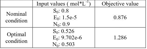
[image:6.595.42.293.516.600.2]set to 1000, which is the time when the maximum Q should be attained. This problem is solved by SQP method, where the simulation result is shown in Table 4. It can be seen that through the process design, the objective is increased nearly 50% over that with nominal condition. In addition, the input values obtained from process design is totally different from that determined by OED methods. Therefore, it is reasonable to integrate parameter estimation with process optimization so that the model identification process can be more focussed on the interesting region of state space.
Table 4 Simulation result of process optimization
Input values ( mol*L-1) Objective value
Nominal condition
S0: 0.8
E0: 1.5e-5
N0: 0.9
0.876
Optimal condition
S0: 0.526
E0: 9.702e-6
N0: 0.503
1.286
5. CONCLUSIONS
In this work, we consider the integrated OED for both input design and observation design. To solve this complex high-dimensional optimisation problem, a two-loop optimisation procedure is proposed, in which the relatively easy observation design is processed in the inner loop, and the input signal is calculated in the outer loop with a stochastic searching mechanism. The computational efficiency is effectively increased.
This new design algorithm has been applied to an enzyme kinetically controlled synthesis process. From the observation design, it is suggested that the state variables Q and S provide
the most informative experimental data than the other measurable variables for those important parameters to be estimated. From the sampling time design, it can be seen that measurement should be taken in the early reaction stage and in the middle reaction for S, and in the late reaction for Q, respectively. The OED result of all design factors is in agreement with the observation design result in terms of the measurement set selection – Q and S are selected in both cases. The sampling strategy is different when the input design is also considered, where the measurement of S is only required in the early reaction stage. With the integrated OED, the parameter estimation uncertainties of those three key parameters are all reduced to a level below 5%. In addition, the process optimization of this kinetic process is also investigated, from which the production rate of Q is largely increased.
The proposed algorithm provides a computationally efficient framework for integrated OED. It has been shown capable of handling the case study enzyme reaction system. Further investigations will be made to improve its function to more complex systems such as systems with large model uncertainties or systems with time-varying input factors.
REFERENCES
Atkinson, A.C., Fedorov, V.V., Herzberg, A.M., and Zhang, R. (2014). "Elemental information matrices and optimal experimental design for generalized regression models," J. Statistical Planning and Inferece, vol. 144, pp. 81-91. Balsa-Canto, E., Alonso, A.A., and Banga, J.R. (2008).
"Computational procedures for optimal experimental design in biological systems". IET Syst. Biology 2(4), 163-172.
Baltes, M., Schneider, R., Sturm, C., and Reuss, M. (1994). "Optimal Experimental Design for Parameter Estimation in Unstructured Growth Models," Biothecnol. Progr., vol. 10, pp. 480-488.
Banga, J.R., Versyck, K.J., and Van Impe, J.F. (2002). "Computation of Optimal Identification Experiments for Nonlinear Dynamic Process Models: a Stochastic Global Optimization Approach," Ind. Eng. Chem. Res., vol. 41, pp. 2425-2430.
Bauer, I., Bock, H.G., Körkel, S., and Schlöder, J. (1999). "Numerical methods for initial value problems and derivative generation for DAE models with application to optimum experimental design of chemical processes," Sci. Comput. in Chemi. Eng. II, vol. 2, pp. 282-289. Bauer, I., Bock, H.G., Körkel, S., and Schlöder, J.P. (2000).
"Numerical methods for optimum experimental design in DAE systems," J. Comp. Applied Math., vol. 120, pp. 1-25.
Boyd, S., and Vandenberghe, L. (2004). Convex optimization: Cambridge university press.
Brown, M., He, F., and Yeung, L.F. (2008). "Robust measurement selection for biochemical pathway experimental design," Int. J. Bioimformat. Res. Appl., vol. 4, pp. 400-416.
in Systems Biology," SIMULATION, vol. 79, pp. 717-725.
Franceschini, G., and Macchietto, S. (2008). "Model-based design of experiments for parameter precision: State of the art," Chem. Eng. Sci., vol. 63, pp. 4846-4872. He, F., Brown, M., and Yue, H. (2010). "Maximin and
Bayesian robust experimental design for measurement set selection in modelling biochemical regulatory systems," Int. J. Robust Nonlin., vol. 20, pp. 1059-1078. Hosten, L.H. (1974). "A sequential experimental design
procedure for precise parameter estimation based upon the shape of the joint confidence region," Chem. Eng. Sci., vol. 29, pp. 2247-2252.
Kutalik, Z., Cho, K.-H., and Wolkenhauer, O. (2004). "Optimal sampling time selection for parameter estimation in dynamic pathway modeling," Biosyst., vol. 75, pp. 43-55.
Liepe, J., Filippi, S., Komorowski, M., and Stumpf, M.P.H. (2013). "Maximizing the Information Content of Experiments in Systems Biology," PLoS Comput. Biol., vol. 9, p. e1002888.
Ljung, L. (1987). "System identification: theory for the user," Preniice Hall Inf. and System Sciencess Series,, vol. 7632,
Motulsky, H., and Christopoulos, A. (2004). Fitting models to biological data using linear and nonlinear regression: a practical guide to curve fitting: Oxford University Press.
Peleg, M., Yeh, I., and Altman, R.B. (2002). "Modelling biological processes using workflow and Petri Net models," Bioinformatics, vol. 18, pp. 825-837.
Walter, E., and Pronzato, L. (1990). "Qualitative and quantitative experiment design for phenomenological models—A survey," Automatica, vol. 26, pp. 195-213. Yao, K.Z., Shaw, B.M., Kou, B., McAuley, K.B., and Bacon,
D.W. (2003). "Modeling Ethylene/Butene
Copolymerization with Multi‐site Catalysts: Parameter
Estimability and Experimental Design," Polymer Reaction Eng., vol. 11, pp. 563-588.
Yu, H., Yue, H., and Halling, P. (2015). "Optimal Experimental Design for an Enzymatic Biodiesel Production System," IFAC, vol. 48, pp. 1258-1263. Yue, H., Halling, P., and Yu, H. (2013)."Model development