Alternative measurement configurations
for extracting bulk optical properties
using an integrating sphere set-up
Suresh N. Thennadil
1*and Yi-chieh Chen
21School of Engineering and Information Technology, Charles Darwin University,
Darwin, Australia
2Department of Chemical and Process Engineering, University of Strathclyde, Glasgow,
United Kingdom
Abstract
The usual approach for estimating bulk optical properties using an integrating sphere measurement set-up is by acquiring spectra from three measurement modes namely collimated transmittance (Tc), total transmittance (Td) and total diffuse reflectance (Rd) followed by the
inversion of these measurements using the adding-doubling method. At high scattering levels, accurate acquisition of Tc becomes problematic due to the presence of significant amounts of
forward scattered light in this measurement which is supposed to contain only un-scattered light. In this paper, we propose, and investigate the effectiveness of using, alternative sets of integrating sphere measurements that avoid the use of Tc and could potentially increase the upper limit of
concentrations of suspensions at which bulk optical property measurements can be obtained in Visible-Near-infrared (VIS-NIR) region of the spectrum. We examine the possibility of replacing Tc with one or more reflectance measurements at different sample thicknesses. We also examine
the possibility of replacing both the collimated (Tc) and total transmittance (Td) measurements
with reflectance measurements taken from different sample thicknesses. The analysis presented here indicates that replacing Tc with a reflectance measurement can reduce the errors in the bulk
scattering properties when scattering levels are high. When only multiple reflectance
measurements are used, good estimates of the bulk optical properties can be obtained when the absorption levels are low. In addition, we examine whether there is any advantage in using 3 measurements instead of 2 to obtain the reduced bulk scattering coefficient and the bulk absorption coefficient. This investigation is made in the context of chemical and biological suspensions which have a much larger range of optical properties compared to those encountered with tissue.
Keywords
Optical properties, Adding-Doubling method, Inverse Adding-Doubling, Radiative transfer theory, Multiple light scattering, Near-infrared spectroscopy, UV-Vis spectroscopy, Diffuse reflectance, Tissue Optics
*Corresponding author: Suresh N. Thennadil, Charles Darwin University, Purple 12.1.04 Ellengowan Drive, Darwin, NT, 0909,
Australia. Email: suresh.thennadil@cdu.edu.au
Introduction
The estimation of bulk optical properties of chemical and biological suspensions such as blood, cell cultures and latex particle suspensions have been of great interest since, they lead to better understanding of light propagation through these turbid media thus aiding instrument design as well as developing methods to extract information regarding physical and chemical properties of a sample.1-3A common method for ex-vivo measurement of bulk optical properties of tissue, blood and other types of particle
suspensions, is based on measurements obtained using an integrating sphere set up (ISS) which may consist of a single or double integrating spheres.4-7 Three measurements are taken at each wavelength. These are the total diffuse transmittanceT ( )d , total diffuse reflectance R ( )d and collimated transmittanceT ( )d . These measurements are then inverted, using radiative transfer equation, to extract the bulk absorption coefficient
a( )
, bulk scattering coefficient s( ) and the anisotropy factor g( ) of the sample
over the desired wavelength range. The inverse adding-doubling (IAD) method has been a popular approach for extracting the bulk optical properties where, the adding-doubling method is used iteratively to determine the bulk optical properties.8 There are 2 ways this iterative approach can be used:
Inversion Method 1
This approach is commonly used in the Tissue Optics field and consists of the following steps: The input to the IAD algorithm consists of guess values for the optical depth ( ) and albedo ( ). The anisotropy factor g( ) is given a fixed value. For tissue this is usually set at 0.8.9 Using these inputs, the radiative transfer equation (RTE) is solved using the adding-doubling method to get calculated values of total transmittance
d,calc
T ( )andRd,calc( ) . These values are compared with their experimental
counterpart and, if they are not to within a set tolerance, the guess values are updated and the process repeated iteratively until the calculated and experimental values match. The values of albedo and optical depth are then used to calculate the bulk absorption and scattering coefficients making use of the fact that,
( ) a( ) s( ) (1) and
a s s
( ) ( )
( ) ( ) (2)
's( ) s( ) 1 g( ) (3) is believed to lead to fairly accurate values for the latter parameter and thus is given as the output from the IAD routine in addition to the bulk absorption coefficient. The impact of doing this is examined later.
Using a( )obtained from the previous step and the collimated transmittance measurement, the bulk scattering coefficient is calculated by invoking Beer’s law, rearranging which we get:
s( ) 1ln(T ( ))c a( ) (4)
where is the sample thickness which is known. Now the anisotropy parameter is obtained using Equation (3) and thus all 3 bulk optical parameters are determined.
Inversion Method 2
Another approach1,5,10 is to the let all 3 optical parameters to be estimated as part of the IAD process i.e. the anisotropy factor is not fixed. In this case, the inputs to the IADD are the initial guess values for albedo, optical depth and the anisotropy factor and all the 3 measurements i.e. total transmittance, total reflectance and collimated
transmittance. The results arising from this method compared to Method 1 is discussed later.
For both methods, the use of collimated transmittance poses problems in achieving reasonable accuracy in the estimated bulk optical properties. For a fixed sample thickness, as scattering increases the un-scattered light collected in collimated transmittance mode decreases which in turn decreases the signal-to-noise of the measurement. In addition, there is an increase in the amount of forward scattered light collected in this mode which becomes significant when scattering is high.11
problem of multiple scattered light corrupting collimated transmittance measurements. This poses a limitation in using the ISS for estimating bulk optical properties of chemical suspensions which contain particles at moderate-to-high concentrations with optical properties much higher than those encountered in tissue.
A third effect, which usually occurs at high particle concentrations, is due to the inter-particle interactions becoming significant. In such cases, the particles exhibit ordered structures, as a result of which the independent scattering assumption on which Beer’s law is based on is not valid. The effect of this dependent scattering is to increase the amount of transmitted light due to constructive interference.14,15 This leads to a significant deviation in the calculated collimated transmittance which in turn can lead to large errors in the estimated bulk optical properties.
In light of the factors discussed above, it would be desirable if the collimated transmittance measurement is replaced by an alternative measurement. In this paper, we propose, and investigate the effectiveness of using, alternative sets of integrating sphere measurements that avoid the use of Tc which could potentially increase the upper limit of concentrations of suspensions at which bulk optical property measurements can be obtained in the Vis-NIR region of the spectrum.16 We examine the possibility of
replacing Tc with one or more reflectance measurements at different sample thicknesses. We also examine the possibility of replacing both the collimated (Tc) and total
transmittance (Td) measurements with reflectance measurements taken from different sample thicknesses.
It is also known that accurate determination of the anisotropy factor is difficult using the integrating sphere set-up.2 It may be only possible to obtain the reduced
scattering coefficient with sufficient accuracy. If that is the case, then the natural question is whether we need only 2 measurements namely, Td and Rd and if there is any utility in using more than 2 measurements. Finally, is it possible to use only reflectance
measurements taken from different sample thicknesses to obtain accurate values of the bulk optical properties? These questions will be examined in this paper in the context of chemical and biological suspensions. It should be noted that the requirements for
charactering suspensions from chemical and biochemical processes can be radically different from those required for tissue optical properties due to the different range and magnitude of the optical properties encountered.
Before addressing the questions raised above, a description of the alternative sets of measurements considered in this study and a brief description of implementing the IAD are described in the next section.
Bulk Optical Properties using Alternative Configurations
thicknesses. The bulk optical properties obtained by these measurements were compared with those obtained using the usual combination of Tc, Rd and Td. In all these cases the measurements were inverted using the inverse doubling method. The adding-doubling code previously used and validated5 was modified to output values of R
d at different depths that correspond to measurements of different sample thickness ℓ. The sample thicknesses used in the study were 1, 2 and 4 mm. The measurements at these thicknesses were made by using cuvettes of path lengths 1, 2 and 4mm and the
reflectance measurements corresponding to these sample thicknesses will be referred to as Rd1, Rd2 and Rd3 respectively.
The adding-doubling part of the routine is run for a sample of thickness 4mm and the intermediate depths from the doubling procedure includes calculations of reflectance values for 1 and 2mm thicknesses of the suspension. These values were stored in addition to that calculated for 4mm thickness. This eliminates the need to run the doubling part of the routine separately for each of the sample thicknesses. To each of these values, the effect of glass boundaries due to the cuvette walls are added, thus providing the calculated reflectance values corresponding to samples in cuvettes of different path lengths. The inversion consists of minimising an objective function of the form:
p
i,calc i,exp i 1
F Abs M ( ) M ( )
(5)where Mi,exp( ) is the experimentally obtained value of a measurement in mode i (for example total diffuse reflectance of a sample with thickness 1mm), Mi,calc( ) is the value for the corresponding measurement obtained using the adding-doubling method and p is the number of measurement modes used. The values of the bulk optical properties that minimise the objective function Fare taken as the estimates of these properties.
The calculations were carried out using MATLAB® version R2012b. The inversion step utilised the MATLAB function for nonlinear constrained optimization (function “fmincon” in MATLAB optimisation toolbox). For all the measurement configurations considered, inversion method 2 was used, i.e. all three bulk optical parameters are simultaneously determined using 3 or more measurements. These are compared with the inversion method 2 for the specific set of measurements involving Td, Rd and Tc. The iteration procedure is similar for both inversion methods.
For the first wavelength of each sample, initial guess values for albedo, optical depth and anisotropy parameter (fixed value if using Inversion Method 1) were given, and a soft constraint (Upper Bound < Parameter < Lower bound) was applied to each of the optical parameters. Once the solution converged, the estimated values were used as the initial guess values for the next wavelength, and the soft constraints for the
wavelengths can result in convergence issues as well as increase the number of iterations and thus computing time, needed to achieve convergence. As the measurements are taken at small wavelength intervals (4nm), the change in optical properties from one
wavelength to the next will be relatively small and thus using the estimates for the
previous wavelength as initial guess values for the current wavelength can be expected to provide a starting point which is closer to the solution.
In this study, the lower and upper bounds for the soft constraints were set as 0.5 and 1.5 times the guess value respectively. These were found to be sufficient in providing the necessary variation in the searched solution space to account for situations where significant changes in the parameters occur over a short wavelength range such as around absorption peaks. The same setting for initial guess values and boundary conditions mentioned above were used throughout all combinations of input measurements. It should be noted that for the anisotropy factor, setting the upper bound in the above manner could result in the bound being greater than 1 which, could potentially result in
g( ) greater than 1. While the upper bound can be then further constrained to ensure that it is never greater than 1, this was not done in this study. For the calculations reported here this did not adversely affect the convergence and the values never exceeded 1.
Experiments
Optical measurements
Measurements from different measurement modes i.e. collimated transmittance, total diffuse transmittance and total diffuse reflectance were made using a Cary 5000 spectrometer equipped with an external diffuse reflectance accessory (DRA-2500). The measurement set-up is the same as that used in earlier work1,2 except for one
modification. In previous studies, a sample window of 12mm×34mm was employed for collecting all three types of spectra. To utilize the larger reflectance port size (1.5 inch in diameter) of the DRA-2500, cuvette holders for each of the path lengths used in this study were designed to maximize sample exposure area by increasing the sample window size to 29mm×34mm. Tests indicated that this enlarged window size reduced the amount of light loss when taking diffuse reflectance measurements. For all measurement modes, the spectra were collected using a 1s integration time with 4 nm wavelength interval over a wavelength range of 350 – 1850 nm. Three replicates were taken and averaged prior to analysis.
The estimation of optical properties by the standard set of measurements i.e. Tc, Td and Rd was done with measurements made using a 1mm path length cuvette. For the two alternative methods considered here, the required reflectances at multiple (two or more) sample thicknesses were obtained using two cuvettes of path length 2mm and 4mm in addition to the 1 mm path length measurement. The diffuse transmittance
Two types of turbid samples were used in this study: 10 wt% of polystyrene suspension (Thermo Scientific, USA) with particle diameter of 430nm, and Intralipid 20% (Fresenius Kabi, UK) containing 20 wt% of emulsified soya oil. The polystyrene suspension was used at 2 concentrations namely 10%, which was concentration of the purchased product and was used as such and 0.15% which was prepared by diluting the 10% sample with deionized water. 1, 2, 4, 8 and 10wt% intralipid samples were prepared by diluting the purchased 20% Intralipid using deionized water.
Simulations
The theoretical values were calculated using Mie theory to obtain the scattering and absorption cross-sections of a single particle as well as the anisotropy factor. The cross-sections are used to generate the bulk absorption and scattering coefficients by using the volume fraction contribution of all components on the bulk optical properties. The bulk optical properties, together with the anisotropy factor and the refractive index of the cuvette walls, form the inputs to the adding-doubling routine for calculating the simulated spectra. The complex refractive index of polystyrene particles needed for the Mie calculations were taken from earlier work.10
Results and discussion
Polystyrene-water data
In emulsion polymerization reactions, the particle concentration ranges from 0 at the beginning to around 40%. Similarly, the particle diameter will typically range from 0 up to about 1 micron for emulsion polymerization depending on product requirements. Also, product specifications for different batches of product can be vastly different particularly in the requirement of final particle size of the particle. Thus, we can expect the bulk optical properties of the sample to vary widely both during a reaction and from one batch to another. In order to get an understanding of the range over which these properties vary for typical situations, the bulk optical properties of polystyrene in water system was calculated. Figure 1 shows the simulated bulk optical properties of
polystyrene-water suspensions for particle diameter ranging from 100 – 500 nm over the concentration range of 1 – 40%).
It can be seen that the relative change in the bulk absorption coefficient is fairly small (Figure 1(a)), while the reduced bulk scattering coefficient (Figure 1(b)) varies strongly with particle size and concentration with over an order of magnitude difference between the extreme values at the shorter wavelengths. Similarly, the anisotropy factor shows large variations related to particle size (Figure 1(c)). It should be noted that the impact of particle size is not only in terms of magnitude but also the shape of the
Figure 1. Simulated bulk optical properties of polystyrene-water with concentrations spanning particle concentrations of 1 – 40% and particle radius of 100 – 500nm.
400 600 800 1000 1200 1400 1600 1800 0 0.5 1 1.5 2 2.5 3 3.5
Wavelength / nm
A b so rp ti o n C o ef fi ci en t / m m -1 1 % 5 % 10 % 20 % 30 % 40 %
400 600 800 1000 1200 1400 1600 1800
0 50 100 150 200 250 300 350 400
Wavelength / nm
R ed u ce d S ca tt er in g C o ef fi ci en t / m m -1 100 nm 200 nm 300 nm 400 nm 500 nm
400 600 800 1000 1200 1400 1600 1800
0 0.1 0.2 0.3 0.4 0.5 0.6 0.7 0.8 0.9 1
Wavelength / nm
For human skin, the variation in the reduced scattering coefficient was found to be between 0.3 to 1.6 mm-1 for skin samples from different locations in the body at around 1000 nm,9 which is exceeded by the polystyrene-water system at around 1% particle concentration. In addition, comparing the variations in skin optical properties with Figure 1, it can be seen that the values are much smaller than would be encountered in emulsion polymerization reactions. A similar study, with apple skin and tissue, showed that the reduced scattering coefficients of apple skin and tissue from a variety of cultivars have reduced scattering coefficients with relatively small variations with the reduced scattering coefficient of apple skin in the region of 25 mm-1 at 400nm while the flesh has much lower value (around 4 – 5 mm-1).5 Thus the magnitude and range of the reduced
scattering coefficients normally encountered in emulsion and suspension polymerization processes is much higher than in tissue systems.
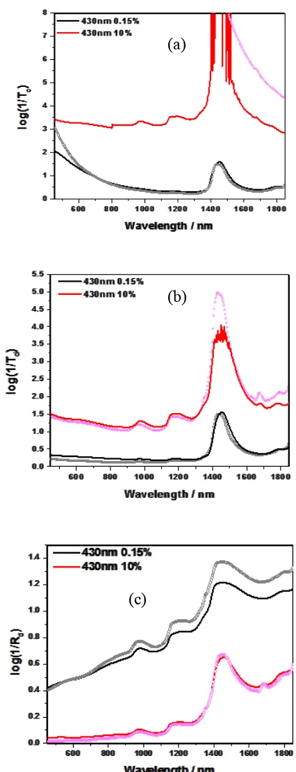
Figure 2 compares the experimental and simulated Tc, Td and Rd for polystyrene-water suspensions at 2 particle concentrations. The problem with obtaining accurate measurements of collimated transmittance when particle concentration is high is clearly evident in Figure 2(a) where the y axis is in Optical Density (OD) units. The theoretical OD values of collimated transmittance measurements indicates a sharply increasing trend with decreasing wavelength as would be expected since, the magnitude of scattering increases sharply with decreasing wavelengths. However, the corresponding experimental OD values are almost flat at the shorter wavelengths indicating that a significant amount of forward scattered light is included in the measurement. Thus, the error in the measured un-scattered transmitted light is extremely high even at concentrations that are moderate in terms of suspensions encountered in chemical industries.
For Td, there is good agreement between theoretical and experimental values as can be seen in Figure 2(b). The experimental OD values are slightly higher compared to the calculated values in the shorter wavelength (high scattering) region while they are lower than the calculated values at the longer wavelength region around and beyond the water absorption peak where absorption is the dominant effect. The difference between the experimental and simulated Td is larger for the higher concentration sample, in particular in the stronger absorption spectral region. On the contrary, Rd shows a larger difference between measured and calculated values for the sample with smaller particle concentration.
Figure 2. Comparison of simulated and measured spectra ((a) Tc (b) Td, (c) Rd) of polystyrene suspensions of particle size of 430 nm, 0.15 and 10 % particle concentration by weight. Spectra simulated using Mie calculation is are pink (10%) and grey (0.15%), while the measured spectra are in red and black respectively.
(a)
(b)
Inversion Method 1
First we consider the extraction of a( )and 's( )which is the first step of Inversion Method 1. We examine the effect of the value at which g( ) is fixed. The bulk absorption and reduced scattering coefficients obtained from the inversion using different values of anisotropy factor are shown in Figure 3.
Figure 3. Bulk optical properties ((a) μs , and (b) μs′) of polystyrene suspension of particle diameter 430 nm and 10 % by weight particle concentration. Values obtained by
(a)
[image:11.612.157.462.199.673.2]inverting the experimental data by fixing g at different values is compared to the theoretical value obtained from Mie calculations.
From Figure 3(a), it can be seen that when g( ) is fixed at value within 0.7 – 0.9, the results are very similar except at the lower end where slight differences can be seen. Further the overall profile of the extracted 's( )is very similar to the calculated values. However, when the value is set to 0.6, 's( ) becomes highly inaccurate both in terms of magnitude and profile. This indicates that while there is some flexibility in fixing the value of the anisotropy factor, there is a relatively narrow range within which reliable estimates of 's( )can be obtained. In tissue, this is not a big problem since, as
mentioned earlier, the variations of the optical properties from sample to sample are fairly low. For chemical suspensions, the large variations in particle size would mean that a-priori knowledge is usually not available to facilitate the fixing of the anisotropy factor to an appropriate level and a trial and error approach would be required. This would not be conducive to rapidly characterizing the samples, which is essential for process monitoring purposes. It should be noted that a( )is not appreciably affected by the value chosen for the anisotropy factor. If s( )is to be extracted by invoking Equation (3) and by inserting the value to which g( ) was fixed, the results will be severely off the mark as seen in Figure 3(b).
This analysis suggests that the fixed-g approach could be useful for cases where there is no need for obtaining s( )and g( ) separately. It however would require that the sample-to- sample changes in the anisotropic factor is small or the range of values which would allow for the accurate convergence of the solution is known.
The anisotropy factor g( ) can be obtained by substituting the value of s( )
obtained from Equation (4) into Equation (3) and solving forg( ) . The values so obtained are shown in Figure 4. For a particle concentration of 0.15% it is seen from Figure 4(a), that there is qualitative agreement in terms of the profile of the anisotropy factor with the values being underestimated as the shorter wavelengths up to about 1200 nm. Above this wavelength, the values are overestimated and the profile looks erratic. At 10% particle concentration, the estimated g( ) is negative and the profile is the opposite that of the calculated values. In other words, the values are quantitatively and
qualitatively erroneous. This analysis indicates that the Inversion method 1 is not
Figure 4. Anisotropic factor g(λ) obtained by using Equation (4) is compared to the values obtained from Mie calculations for (a) 0.15% and (b) 10% by weight polystyrene suspensions of particles with diameter of 430nm.
Inversion Method 2
As mentioned previously, this method differs from Method 1 in that, all the 3 optical parameters are estimated simultaneously with all the measurements input into the IAD at the same time. Four sets of measurements are considered here. The first set
600 800 1000 1200 1400 1600 1800 0.1
0.2 0.3 0.4 0.5 0.6 0.7 0.8 0.9
Wavelength / nm
g
Calculated from Tc Calculated from Mie
600 800 1000 1200 1400 1600 1800 -5
-4 -3 -2 -1 0 1
Wavelength / nm
g
Calculated from Tc Calculated from Mie
(a)
(Configuration 1) uses the same set of measurements as used by Inversion Method 1 namely Tc, Td and Rd with all measurements made with a sample thickness of 1mm. Configuration 2 replaces Tc with a reflectance measurement: Td, Rd1, and Rd3. Here Rd1 refers to total diffuse reflectance taken using a sample of thickness 1mm and Rd3 refers to the total diffuse reflectance measurement made with a sample thickness of 4mm.
Configuration 3 consists of Td, Rd1, Rd2 and Rd3 where Rd2 indicates total diffuse reflectance taken with a 2mm sample thickness. Finally, using only reflectance
[image:14.612.118.530.194.529.2]measurements (Rd1, Rd2 and Rd3) was considered and is referred to as Configuration 4.
Figure 5. Bulk optical properties of 10% polystyrene suspension containing 430nm
diameter particles calculated using different sets of measurement modes and inversion method 2. a) μ𝑎 (Note: The red line is not visible as it is overlapped by the green line), (b) g, (c) μs and (d) μs′. The values obtained from Mie calculations are shown for comparison.
From Figure 5(a) it is seen that a(), extracted by replacing collimated transmittance with a reflectance measurement on a sample of different thickness (i.e. Configuration 2), is almost indistinguishable from that obtained using the conventional combination (i.e. Configuration 1). It should be also noted that a()obtained from using Inversion Method 1 is indistinguishable from that obtained using Configuration 1 in conjunction with Method 2 (Data not shown).
600 800 1000 1200 1400 1600 1800 0 10 20 30 40 50 60 70 80 Mie
Tc + Td + Rd1 Td + Rd1 3 Td + Rd1 2 3 Rd1 2 3
s
'
Wavelength / nm
600 800 1000 1200 1400 1600 1800 0.0 0.2 0.4 0.6 0.8 1.0 Mie
Tc + Td + Rd1 Td + Rd1 3 Td + Rd1 2 3 Rd1 2 3
g
Wavelength / nm
600 800 1000 1200 1400 1600 1800 0 100 200 300 400 500 Mie
Tc + Td + Rd1 Td + Rd1 3 Td + Rd1 2 3 Rd1 2 3
s
Wavelength / nm
600 800 1000 1200 1400 1600 1800 0.0 0.5 1.0 1.5 2.0 2.5 3.0 3.5 a
Wavelength / nm
Mie
Tc + Td + Rd1 Td + Rd1 3 Td + Rd1 2 3 Rd1 2 3
(b)
(d) (a)
It was found that the combination Td, Rd1 and Rd2 (instead of Rd3 which was used in Configuration 2) leads to convergence problems due to the small differences in
reflectance spectra from the 1mm and 2mm path length cuvettes (not shown). It should be noted that the specular reflectance from the air-cuvette-sample boundary makes up a large portion of the reflected signal. The change in the reflectance due to the change in sample thickness going from 1 mm to 2 mm thickness is relatively small compared to specular reflectance. As a result, it appears there is not sufficient differentiation between the two reflectance measurements to aid in the separation of absorption and scattering effects. This small difference also adversely impacts the convergence of the IAD routine when using Configuration 4 measurements (i.e. using only the three reflectance
measurements), leading to a very large deviation in the estimated a()for wavelengths greater than about 1300nm. In this wavelength region, the absorption is high and
therefore the spectra are dominated by the contribution from specular reflectance which will be the same for all three samples. The use of more than 2 diffuse reflectance measurements (Configuration 3) does not lead to any significant improvement over Configuration 2, which is expected given our earlier observations regarding the use of the combination of Rd1 and Rd2.
Figure 5(b) shows g( ) extracted using the different sets of measurements. It is seen that unlike for Inversion Method 1 (see Figure 4(b)), there is qualitative agreement with the theoretical values in that g( ) decreases with increasing wavelength. There is quantitative agreement at the shorter wavelengths up to about 1000 nm. With increasing wavelength, the magnitude of scattering reduces and the absorption starts to increase. This appears to have an adverse effect with respect to the estimation of the anisotropy factor. This observation is in line with the observations in a previous study2 on bacterial suspensions where it was found that the upper limit of wavelength for which the
estimated g( ) appeared to be realistic, increased with increasing cell concentration i.e. with increasing magnitude of scattering.
In terms of the different sets of measurements, replacing Tc with a reflection measurement (Configuration 2) provides a marked improvement. Configuration 2, which uses 1 reflectance measurement, provides better agreement with theory than
Configuration 3 where 2 reflectance measurements are used in place of Tc in the NIR region above 1000nm. Using only reflectance measurements (Configuration 4) gives similar results as Configurations 2 and 3 up to about 1000 nm above which the lack of differentiation between the different reflectance measurements becomes an issue. Despite this, below 1000 nm, it appears that using Configuration 4 gives better estimates than using Configuration 1 which contains the Tc measurement. Overall the analysis suggests that for higher concentrations, Inversion Method 2 is superior to Method 1 with
significant improvement obtained for Method 2 when Tc is replaced with a reflectance measurement. If very accurate values of anisotropy factor are required neither of the methods are satisfactory.
on the value to which g( ) is fixed. This is not the case in method 2, since the anisotropy factor is not fixed and is estimated along with s( )and thus only a single estimate will result in the application of this method. This is particularly significant because from Figure 3(a), it can be seen that the value will vary widely depending on the value of g( )
and also the wavelength profile of the bulk scattering coefficient can vary significantly when Method 1 is used. Secondly, it can be seen that the profile with respect to
wavelength is appreciably better in a qualitative sense when Method 2 is used.
Comparing the use of different configurations in conjunction with Method 2, it can be seen from Figure 5(c) that replacing Tc with one or more reflectance
measurements (Configurations 2 and 3) leads to significant improvement in the estimation of the bulk scattering coefficient for wavelengths below 1000 nm. Both configuration 2 and 3 exhibits larger errors at shorter wavelengths (below 700nm). At above 1000nm, all the configurations lead to similar values. It can also be seen that Configuration 3 which has an additional reflectance measurement leads to better agreement with theoretical values in the between about 700 – 1000nm. Using only reflectance measurements (Configuration 4) has overall a better performance than
Configuration 1 though it does not perform as well as Configurations 2 and 3 which have Td included in the inversion.
In some cases, where the interest is to follow the overall effect of particle size and concentration, it may be sufficient to examine the combined effect of scattering (i.e. a combination of scattering coefficient and anisotropy factor) through the reduced
scattering coefficient 's( )to monitor the state of a particulate sample. So the impact of using the different sets of measurements on the estimated values of 's( )is examined here.
Figure 5(d) shows 's( )extracted using the different sets of measurements. First we compare these results with that when Inversion Method 1 is used (Figure 3(b)). It can be seen that the magnitude of 's( )obtained with Method 1 is almost indistinguishable from that obtained with Inversion Method 2 when Configuration 1 is used. In other words, the reduced scattering coefficient estimated using only 2 measurements namely Td and Rd is similar to that obtained using 3 measurements Tc, Td and Rd. This indicates, from an accuracy point of view, that the addition of Tc has no impact in the estimation of
' s( )
. However, it should be noted that the first step of Method 1 is reliant on g( )
being fixed to an appropriate value as mentioned in the discussion of the method with the aid of Figure 3(b). Using all the three measurements Rd, Td and Tc together, as done by Method 2, increases the reliability of the inversion method in that there is no need to fix
g( )and ensure that it falls within the right range.
Examining the other configurations, we see that Configuration 2 and
scattered light due to the high level of multiple scattering. Thus replacing Tc with a reflectance value provides both an increased reliability in terms of convergence of the inversion due to the additional measurement as well as improved accuracy in the high scattering region of the spectrum. Configurations 2 and 3 lead to values which are indistinguishable suggesting that additional reflectance measurements do not lead to improved estimates. When only the three Rd measurements (Configuration 4) are used, the estimated values of 's( )show large deviations from the theoretical values over the entire wavelength range. This appears to be primarily the result of lack of convergence of the inversion. This indicates that a judicious choice of sample thicknesses has to be made so that the reflectance measurements from different sample thicknesses are sufficiently distinguishable.
The analysis with polystyrene-water data suggests that at high scattering
conditions, the replacement of Tc with one or more reflectance measurements can provide improved estimates of the scattering properties s( ) and g( ) . When the combined parameter i.e. 's( )is used, the profile obtained is consistent regardless of whether Tc or the alternative measurements are used. However, quantitatively there is still a marked improvement when Tc is replaced with a reflectance measurement in the shorter wavelengths where scattering is high.
In the next section we will focus only on the performance of the configurations on the estimation of the reduced scattering coefficient 's( ) and also focus only on
Inversion Method 2 in the interest of brevity.
Intralipid Suspension
The spectra of samples of intralipid with concentrations ranging from 1 to 10% by weight of soya oil collected with different measurement modes are shown in Figure 6. As expected, for both types of transmittance measurements, the optical density increases with increase in the concentration of scatterers. The optical density for the reflectance measurements decreases with increasing intralipid concentration since an increase in scattering results in more photons being reflected out through the front end of the sample.
In Figure 6(c), the reflectance measurements with sample thicknesses of 1, 2 and 4 mm are shown. From this figure, it can be seen that the prominent spectral difference between the reflectance measurements with different sample thicknesses (Rd1, Rd2 and Rd3) occurs in the shorter (UV-vis) wavelengths where absorption is low. The samples with low concentrations (1 and 2%) exhibit greater spectral difference between different sample thicknesses than the high concentration ones. Also, it can be seen that at
difference in the OD of reflected light from the three different sample thicknesses. These observations can be explained by considering the effects of absorption and scattering.
Figure 6. (a) Tc, (b) Td, and (c) Rd spectra of intralipid solutions of different
concentrations. Solid lines in (c) are from samples in 1mm path length cell (Rd1). The
(a)
(b)
dotted-dash and dotted lines are from 2mm (Rd2) and 4mm (Rd3) path length cells, respectively.
An increase in sample thickness allows photons which have travelled farther into the sample (which would otherwise have exited out of the sample if the sample was thinner), to be reflected back and exit out of the front end of the sample. This explains the reduction in OD (i.e. increase in reflected intensity) in the samples of 1% and 2%
intralipid with respect to the 4% sample. As the magnitude of absorption increases, the probability that photons from greater distances within the sample will contribute to the reflected intensity will decrease. In other words, the contribution of these photons
[image:19.612.101.483.361.663.2]towards the total reflected intensity will be smaller as absorption increases. This results in smaller differences in the reflected intensity in the NIR region where absorption is much higher than in the UV-Vis region. Also an increase in scattering entities (increase in intralipid concentration) will result in an increase in the number of scattering events experienced by a photon per unit length in the perpendicular direction (i.e. along the direction which thickness is measured) within the sample. This will lead to a greater amount of absorption per unit thickness of the sample. This in turn results in decreasing the probability of photons that have travelled deeper into the sample in contributing to the reflected intensity. Thus the sensitivity of reflected light to sample thickness decreases as the concentration of intralipid increases.
Figure 7. μ𝑎 of different intralipid concentrations inverted using (a) Tc, Td and Rd1, (b)
Td, Rd1 and Rd3, (c) Td, Rd1, Rd2 and Rd3, and (d) Rd1, Rd2 and Rd3 measurements.
400 600 800 1000 1200 1400 1600 1800
0.0 0.5 1.0 1.5 2.0 2.5 3.0 a
Wavelength / nm
Td Rd1 2 3 10 % 8 % 4 % 2 % 1 %
400 600 800 1000 1200 1400 1600 1800
0.0 0.5 1.0 1.5 2.0 2.5 3.0
Tc Td Rd1 10 % 8 % 4 % 2 % 1 % a
Wavelength / nm
400 600 800 1000 1200 1400 1600 1800
0.0 0.5 1.0 1.5 2.0 2.5 3.0 a
Wavelength / nm
Rd1 2 3 10 % 8 % 4 % 2 % 1 %
400 600 800 1000 1200 1400 1600 1800
0.0 0.5 1.0 1.5 2.0 2.5 3.0 a
Wavelength / nm
The values of a( )extracted from the four measurement configurations are shown in Figure 7. Note that for the intralipid dataset the theoretical values (using Mie theory) are not shown. This is due to the large uncertainty in the measurement of the emulsion droplet sizes when using methods such as Dynamic Light Scattering (DLS). This was not a problem with polystyrene latex particles since, good estimates were provided by the manufacturer and DLS and SEM comparisons were made in-house on a number of polystyrene particle sizes which indicated consistency in the measured values.
It can be seen from Figure 7, that the values obtained using configurations 2 and 3 are in good agreement with the conventional set up (configuration 1) over most of the wavelength range considered here except around the water absorption peak around 1430 nm. In this region, the absorption peaks obtained by these configurations appear slightly suppressed compared to configuration 1. In other words, the a( ) in this region are underestimated compared to values obtained from the standard configuration when these two configurations are used. While with the polystyrene data, the configurations 2 and 3 did not exhibit a difference in the estimated properties, for this data set we can see that the addition of an extra reflectance measurement (Rd2) in configuration 3, results in a slight enhancement of the absorption peak around 1430 nm bringing it closer to the values obtained using the conventional set up. Configuration 4, where only the
reflectance modes were used, shows (Figure 7(d)) good agreement with the conventional set up at low absorbance levels. Beyond about 1250nm, the results show a large deviation from the values obtained from the conventional set up. This is expected given that the spectral differences between samples of different thicknesses are very small in this region and thus causing problems in convergence. It may be possible to address this issue by judicious choice of sample thicknesses.
Comparing the standard configuration with configuration 2 (Figure 8(a) and (b) respectively), it can be seen that at the shorter wavelengths 's( ) obtained by
Configuration 2 is slightly greater than when using the standard configuration. Given the observations from the polystyrene data, it can be concluded that the higher value would be closer to the true value of the coefficient. Also it should be noted that 's( ) are about two times higher for the 10% polystyrene than for the intralipid data. This suggests that when the magnitude of scattering becomes higher we can expect that replacing Tc with a reflectance measurement will provide more accurate estimates.
Figure 8. Reduced bulk scattering coefficients (μs′) of different Intralipid concentrations inverted using (a) Tc, Td and Rd1, (b) Td, Rd1 and Rd3, (c) Td, Rd1, Rd2 and Rd3, and (d) Rd1, Rd2 and Rd3 measurements.
Conclusions
This study indicates that when scattering levels are high, more accurate estimates of the scattering parameters s( ), g( ) and 's( ) can be obtained by replacing the collimated transmittance measurement with a reflectance measurement using a different sample thickness. Further improvements are sometimes possible using additional sample thicknesses provided there is sufficient discrimination between reflectances from
different thicknesses.
It was also seen that, Inversion Method 1 which is commonly used in
characterizing tissue, leads to inferior estimates of s( )and g( ) compared to Inversion Method 2 when particle concentrations are high such as those encountered in emulsion
400 600 800 1000 1200 1400 1600 1800 0 5 10 15 20 25 30 35 40
Tc Td Rd1 10 % 8 % 4 % 2 % 1 % s '
Wavelength / nm
400 600 800 1000 1200 1400 1600 1800 0 5 10 15 20 25 30 35 40
Td Rd1 3 10 % 8 % 4 % 2 % 1 % s '
Wavelength / nm
400 600 800 1000 1200 1400 1600 1800 0 5 10 15 20 25 30 35 40
Rd 1 2 3 10 % 8 % 4 % 2 % 1 % s '
Wavelength / nm
400 600 800 1000 1200 1400 1600 1800 0 5 10 15 20 25 30 35 40
Td Rd1 2 3 10 % 8 % 4 % 2 % 1 % s '
Wavelength / nm
(a) (b)
polymerization. If only 's( )is required, then using Inversion method 1 which requires only 2 measurements can provide similar performance as Inversion Method 2 which requires at least 3 measurements as long as the scattering levels are low. Even in this scenario, the extra measurement affords greater flexibility and reliability since it allows us to circumvent the need for fixing g( ) within an appropriate range. Ensuring that it falls in an appropriate range can be problematic in the case of monitoring of emulsion and suspension polymerization reactions where the particle sizes and concentrations vary widely both within a batch and between batches. The values of a( ) estimated using the two configurations are practically indistinguishable.
In practical situations, particle volume fractions can be as high as 40%. At such high particle volume fractions, it might also not be possible to obtain adequate signal from diffuse transmittance measurements. In such cases, it would be desirable if only diffuse reflectance measurements from different sample thicknesses (Configuration 4) can be used. This study indicates that at low levels of absorption, this configuration can provide estimates of a( ) with good accuracy. For this configuration, 's( ) is underestimated when the scattering levels are higher. Analysis indicates that this issue arises when the reflectance measurements at the different thicknesses are not sufficiently distinct. The sample thicknesses in this study were arbitrarily chosen (based on the availability of cuvettes with different path lengths). It may be possible to address this problem of lack of differentiation in the reflectance spectra by judicious choice of sample thickness. This might require the use of a variable path length sample cell,16 which is designed to provide flexibility in the choice of sample thicknesses, so that the
measurements can be optimized.
Funding
The authors wish to acknowledge funding from the University of Strathclyde and Scottish Enterprise Proof of Concept Programme.
References
1. R. Steponavicius, S.N. Thennadil. “Full Correction of Scattering Effects by Using the Radiative Transfer Theory for Improved Quantitative Analysis of Absorbing Species in Suspensions”. Appl. Spectrosc. 2013. 67(5): 526-535.
3. M.A. Velazco-Roa, E. Dzhongova, S.N. Thennadil. “Complex refractive index of non-spherical particles in the vis-NIR Region – Application to Bacillus Subtilis
spores”. Appl. Opt. 2008. 47 (33): 6183-6189.
4. J.W. Pickering, S.A. Prahl, N.v.W Wieringen, J.F. Beek, H.J.C.M. Sterenborg.
Double-integrating-sphere system for measuring the optical properties of tissue. Appl. Opt. 1993. 32(4): 399-410.
5. W. Saeys, M.A. Velazoc-Roa, S.N. Thennadil, H. Ramon, B.M. Nicolai. “Optical properties of apple skin and flesh in the wavelength range from 350 to 2200 nm”. Appl. Opt. 2008. 47(7): 908-919.
6. M. Friebel, A. Roggan, G. Muller, M. Menke. “Determination of optical properties of human blood in the spectral range 250to1100nm using Monte Carlo simulations with hematocrit-dependent effective scattering phase functions”. J. Biomed. Opt. 2006. 11(3): 034021-1 - 10.
7. L. Wang, S. Sharma, B. Aernouts, H. Ramon, W. Saeys. “Supercontinuum laser based double-integrating-sphere system for measuring optical properties of highly dense turbid media in the 1300-2350nm region with high sensitivity”. Proc. SPIE 8427, Biophotonics: Photonic solutions for better health care III, 84273B. 2012. Doi: 10.1117/12.922491.
8. S.A. Prahl. “The Adding-Doubling Method”. In: A.J. Welch, M.J.C.v. Gemert, editors. Optical Thermal Response of Laser Irradiated Tissue. Plenum Press: New York, 1995. Pp. 101-129.
9. T.L. Troy, S.N. Thennadil. “Optical properties of human skin in the near infrared wavelength range of 1000 to 2200 nm”. J. Biomed. Opt. 2001. 6(2): 167-176.
10.R. Steponavicius, S.N. Thennadil. “Extraction of chemical information of suspensions using radiative transfer theory to remove multiple scattering effects: Application to a model two-component system”. Anal. Chem. 2009. 81(18): 7713-7723.
11.L. Wind, W.W. Szymanski. “Quantification of scattering corrections to the Beer-Lambert law for transmittance measurements in turbid media”. Meas. Sci.Technol. 2002. 13(3): 270-275.
12.Swanson, N.L., B.D. Billard, and T.L. Gennaro. “Limits of optical transmission measurements with application to particle sizing techniques”. Appl. Opt. 1999. 38(27): 5887-5893.
13.B. Aernouts, E. Zamora-Rojas, R.V. Beers, R Watte, L. Wang, M. Tsuta.
“Supercontinuum laser based optical characterization of Intralipid phantoms in the 500-2250 nm range”. Opt. Exp. 2013. 21(26): 32450-32467.
14.V.P. Dick. “Applicability limits of Beer's law for dispersion media with a high concentration of particles”. Appl. Opt. 1998. 37(21): 4998-5004.
15.V. Twersky. “Transparency of pair-correlated, random distributions of small scatterers, with applications to the cornea”. J. Opt. Soc. Am. 1975. 65(5): 524-530. 16.S.N. Thennadil, Y.-C. Chen. “Apparatus and method for estimating bulk optical