City, University of London Institutional Repository
Citation
:
Bianchini, D., Castro Alvaredo, O. & Doyon, B. (2015). Entanglement entropy of non-unitary integrable quantum field theory. Nuclear Physics B, 896(July 2), pp. 835-880. doi: 10.1016/j.nuclphysb.2015.05.013This is the accepted version of the paper.
This version of the publication may differ from the final published
version.
Permanent repository link: http://openaccess.city.ac.uk/12202/
Link to published version
:
http://dx.doi.org/10.1016/j.nuclphysb.2015.05.013Copyright and reuse:
City Research Online aims to make research
outputs of City, University of London available to a wider audience.
Copyright and Moral Rights remain with the author(s) and/or copyright
holders. URLs from City Research Online may be freely distributed and
linked to.
Entanglement Entropy of Non-Unitary Integrable Quantum Field Theory
Davide Bianchini•, Olalla A. Castro-Alvaredo• and Benjamin Doyon◦
• Department of Mathematics, City University London, Northampton Square EC1V 0HB, UK ◦ Department of Mathematics, King’s College London, Strand WC2R 2LS, UK
In this paper we study the simplest massive 1+1 dimensional integrable quantum field the-ory which can be described as a perturbation of a non-unitary minimal conformal field thethe-ory: the Lee-Yang model. We are particularly interested in the features of the bi-partite entangle-ment entropy for this model and on building blocks thereof, namely twist field form factors. Non-unitarity selects out a new type of twist field as the operator whose two-point function (ap-propriately normalized) yields the entanglement entropy. We compute this two-point function both from a form factor expansion and by means of perturbed conformal field theory. We find good agreement with CFT predictions put forward in a recent work involving the present au-thors. In particular, our results are consistent with a scaling of the entanglement entropy given by ceff
3 log` whereceff is the effective central charge of the theory (a positive number related to
the central charge) and`is the size of the region. Furthermore the form factor expansion of twist fields allows us to explore the large region limit of the entanglement entropy and find the next-to-leading order correction to saturation. We find that this correction is very different from its counterpart in unitary models. Whereas in the latter case, it had a form depending only on few parameters of the model (the particle spectrum), it appears to be much more model-dependent for non-unitary models.
March 5, 2015
1
Introduction
Entanglement is a fundamental property of quantum systems which relates to the outcomes of local measurements: performing a local measurement may affect the outcome of local mea-surements far away. This property represents the single main difference between quantum and classical systems. Technological advances have taken entanglement from a strange quantum phenomenon to a valuable resource at the heart of various fields of research such as quantum computation and quantum cryptography. There has also been great interest in developing ef-ficient (theoretical) measures of entanglement, not just in view of the applications above but also as a means to extract valuable information about emergent properties of quantum states of extended systems. One such measure for many-body quantum systems is the bi-partite entan-glement entropy (EE) [1], which we will consider here. Other measures of entanentan-glement exist, see e.g. [1, 2, 3, 4, 5], which occur in the context of quantum computing, for instance. In its most general understanding, the EE is a measure of the amount of quantum entanglement, in a pure quantum state, between the degrees of freedom associated to two sets of independent observables whose union is complete on the Hilbert space. In the present paper, the two sets of observables correspond to the local observables in two complementary connected regions, A
and ¯A, of a 1+1-dimensional (1 space + 1 time dimension) extended quantum model, and we will consider cases where the quantum state is the ground state of a non-unitary, near-critical model.
Prominent examples of extended one-dimensional quantum systems are quantum spin chains. Their entanglement has been extensively studied in the literature [6, 7, 8, 9, 10, 11, 12, 13, 14]. These examples however all refer to unitary quantum spin chains. Interesting examples of non-unitary spin chain systems exist, for instance the famous quantum group invariant integrable XXZ spin chain, with generically non-Hermitian boundary terms; in the thermodynamic limit it has critical points associated with the minimal models of conformal field theory (CFT), including the non-unitary series [15, 16, 17, 18]. Another example is provided by the Hamiltonian studied by von Gehlen in [19, 20]: the Ising model in the presence of a longitudinal imaginary magnetic field. This Hamiltonian has a critical line (in the phase space of its two couplings) which has been identified with the Lee-Yang non-unitary minimal model of CFT, with central chargec=−22/5 [21, 22]. In all these examples, the local, extended Hamiltonians are non-Hermitian, yet have
real and bounded energy spectra. Their critical points are described by CFT models containing non-unitary representations of the Virasoro algebra with real weights, and whose ground states are not the conformal vacua, but negative-weight modules.
annealing [38].
At quantum critical points, the scaling limit of the EE has been widely studied within unitary models of CFT [39, 40, 7, 8, 41, 42]. In particular, the combination of a geometric description, Riemann uniformization techniques and standard expressions for CFT partition functions is very fruitful. Recently [43], this was generalized to non-unitary CFT, where a general formula was obtained using such techniques. Near critical points, the scaling limit is instead described by massive quantum field theory (QFT), and geometric techniques relying on conformal mappings break down. As was found in [44, 45, 46], the most powerful way of studying the EE in unitary models of QFT is using an approach based on local branch-point twist fields. However, the question of the EE in non-unitary near-critical models is much more delicate, and standard arguments give little indications as to how to modify the field-theoretical approach. Importantly, the rigorous derivation presented in [43] provided a precise local-field description of the EE involving composite fields in the branch-point twist family, thus opening the door to its study in non-unitary QFT. In the present paper, using techniques of integrable QFT, we will study the scaling limit of the EE in the near-critical region of von Gehlen’s model, described by the Lee-Yang QFT model.
This paper is organized as follows. In section 2 we recall the main definitions and techniques, and provide a summary of our main results. In section 3 we introduce the Lee-Yang model and some general results on the form factor expansion of correlation functions, their logarithms and expectation values of local fields. In section 4 we review the twist field form factor equations and present solutions for the branch-point twist fields fields T and : Tφ : in the Lee-Yang model. In section 5 we test our form factor solutions by performing a form factor expansion of the functions logh:Tφ:i−2h:Tφ: (r) : ˜Tφ: (0)i and loghT i−2hT(r) ˜T(0)i and recovering the
behaviours−4x:Tφ:log(mr) and−4xT log(mr) for some constantsxT,x:Tφ:which we compare to
CFT predictions. In section 6 we compare a form factor computation of the two-point functions above with a computation in zeroth order conformal perturbation theory. As a byproduct, we find general formulae for some of the CFT structure constants entering the OPEs of T and ˜T
and of : Tφ: with : ˜Tφ:. In section 7 we present numerical results for the R´enyi entropy near criticality and a detailed computation of the first three leading corrections to saturation of the EE. We find that the next-to-leading order correction to saturation is non-universal. In section 8 we present our conclusions and outlook. In appendix A we explain how the normalization and conformal dimension of the field : Tφ: are fixed by CFT. In appendix B we present a detailed analysis of the one-particle form factor contribution to the two-point functions ofT and :Tφ:. A largenexpansion of this function demonstrates that it provides a very substantial contribution to the power law behaviour of the two-point functions at short distances. In appendix C we present a computation of the three particle form factor of Lee-Yang twist fields. In appendix D we perform a computation of some of the structure constants entering the OPE of fields T
2
General aspects and summary of main results
In order to provide a formal definition of the EE, the Hilbert space of an extended quantum sys-tem, such as a spin chain, is decomposed into a tensor product of local Hilbert spaces associated to its sites. Grouping together sites associated to the regions Aand ¯A, this gives:
H=A ⊗A¯. (1)
The EE in a state|ψiis the von Neumann entropy of the reduced density matrixρAassociated toA:
SA=−TrAρAlogρA , ρA= TrA¯|ψihψ|. (2)
Another frequently used measure of entanglement is the R´enyi entropy,
SA(n) = log TrAρ n A
1−n , (3)
which specializes to the von Neumann entropy at n= 1,
lim n→1S
(n)
A =−nlim→1
d dnTrAρ
n
A=SA. (4)
We will study the ground state entanglement entropy in the scaling limit of infinite-length quantum chains. The scaling limit gives the universal part of the quantum chain behaviour near quantum critical points, described by 1+1-dimensional QFT. It is obtained by approaching the critical point while letting the length ` of the region A go to infinity in a fixed proportion with the correlation length ξ (measured in number of lattice sites). If ξ = ∞ from the start, the system is exactly at its critical point, and the scaling limit is described by CFT. In this case the entanglement entropy of unitary critical systems, as a function of `, is divergent in a way which was first understood in [39, 40], numerically confirmed in [7, 8] and generalized and reinterpreted in [41, 42]. The divergency is logarithmic with a proportionality constant depending on the central chargec of the CFT,
SA(n)(`) = c(n+ 1) 6n log
`
ε+o(1), SA(`) = c
3log
`
ε +o(1) (CFT), (5)
and where ε is a non-universal ultraviolet cut-off (proportional to the lattice spacing) which is chosen so as to encode allo(1) corrections. The formulae above are easily adapted to the case of an infinite region `=∞ near criticalityξ <∞, where `is simply replaced by ξ in (5) [41, 42]. In the full scaling limit, where ` and ξ are both large and in proportion to each other, there is a universal scaling function f(`/ξ) which interpolates between the two results,
SA(n)(`) = c(n+ 1) 6n log
`
ε+f(`/ξ) +o(1) (QFT). (6)
We may ask how (if at all) the entanglement entropy is affected by non-unitarity. At criti-cality, it was shown in [43] that the entanglement entropy scales instead as
SA(n)(`) = ceff(n+ 1) 6n log
`
ε+o(1), SA(`) = ceff
3 log
`
ε +o(1) (non-unitary CFT), (7)
where ceff := c−24∆, and ∆ is the smallest (often negative in non-unitary models) scaling
dimension of a primary field in the CFT. For the Lee-Yang model, for example, ceff = 45 as
∆ = −15. This result is not entirely surprising as the work of Itzykson, Saleur and Zuber [47] had previously shown that theeffective central chargeceff also replacescin the expression of the
ground state free energy found by Affleck [48] and Bl¨ote, Cardy and Nightingale [49]. However, the question of the entanglement entropy in non-unitary near-critical models is much more delicate. Importantly, the rigorous derivation of (7) presented in [43] has lead to new insights into the computation of entanglement entropy in non-unitary theories and its field theoretical interpretation, opening the door to its study away from criticality in QFT.
It is known since some time [39, 40, 41, 42] that the bi-partite entanglement entropy in the scaling limit can be re-written in terms of more geometric quantities, using a method known as the “replica trick”. The essence of the method is to “replace” the original QFT model by a new model consisting of ncopies (replicas) of the original one. These are used to represent ρnA
when nis an integer, and then to evaluate TrAρnA. The quantitiesSA andS
(n)
A for generalnare then obtained by “analytic continuation” in n. The matrix multiplications in ρn
A and the trace operation give rise to the condition that the copies be connected cyclically through a finite cut on the regionA. As a consequence, this trace is proportional to the partition functionZn(x1, x2)
of the original (euclidean) QFT model on a Riemann surface Mn,x1,x2 with two branch points, at the pointsx1 andx2 inR2, andnsheets cyclically connected. The positions x1 andx2 of the
branch points are dimensionful positions in the QFT model corresponding to the end-points of the region Ain the scaling limit. This gives:
SA(r) =−lim n→1
d dn
Zn(x1, x2)
Z1n . (8)
Here, r := |x1 −x2| is the euclidean distance between x1 and x2. The above concepts hold,
in principle, for any QFT model, unitary or not. In CFT, one may evaluate this by using the uniformization theorem: the Riemann surface Mn,x1,x2 can be conformally mapped to the
Riemann sphere with two punctures (or the cylinder) by using the mapgreproduced in appendix A.
In the EE context, it was first noticed in [41, 42] that the ratio of partition functions above can be reinterpreted as correlation functions of certain fields, which were not otherwise specified, in unitary CFT. This idea was then generalized to unitary massive theories in [44] and the fields where identified asbranch-point twist fieldsT(x1),T˜(x2) characterized by their non-trivial
exchange relations with other fields of then-copy theory. These twist fields are defined only in the replica model (e.g. they become the identity field whenn= 1), and are primary fields arising from the extra permutation symmetry present in the replica theory; they are associated to the
before their use in the computation of the EE was emphasized, see for instance [50]. In terms of these fields, the replica partition function is given by
Zn(x1, x2)
Z1n =Znε
4∆ThT(x
1) ˜T(x2)i, (9)
wherehT(x1) ˜T(x2)iis a two-point function in the ground state of the replica theory. The
branch-point twist fields are chosen so as to have the CFT normalisation (e.g. the leading term in their OPE has coefficient 1). The constantZn, withZ1 = 1, is ann-dependent non-universal constant,
εis a short-distance cut-off which is scaled in such a way thatdZn/dn= 0 atn= 1, and, finally, ∆T is the conformal dimension of the counter parts of the fields T,T˜ in the underlying n-copy
conformal field theory,
∆T =
c
24
n− 1
n
, (10)
which can be obtained by CFT arguments [50, 42, 44]. It is easy to show that the formula (9) when inserted in (4) indeed reproduces (5) for CFT.
The derivation above assumes unitarity of the theories under consideration. In such case ∆T
is by construction the lowest conformal dimension of any field in the replica theory which has the twist property. The CFT derivation of (5) has been generalized to the non-unitary case in [43] leading to the expressions (7). In this work it was also observed that the EE could be computed from a representation of theZn-orbifold partition function of the theory via correlation functions
involving certain Zn twist fields of then-copy replica theory. This representation requires new twist fields : Tφ : and : ˜Tφ :, obtained from the primary twist fields T and ˜T as leading descendants in the product with the lowest-dimension fieldφ(of conformal dimension ∆). More precisely:
:Tφ: (y) =n2∆−1 lim
x→y|x−y|
2∆(1−1
n)
n X
j=1
T(y)φj(x), (11)
and similarly for : ˜Tφ:. These composite fields were first introduced in [51] and further studied in [52]. The constantn2∆−1 ensures conformal normalization, namely
h:Tφ: (x1) : ˜Tφ: (x2)i=|x1−x2|−4∆:Tφ: (12)
in CFT, where
∆:Tφ:= ∆: ˜Tφ:= ∆T +
∆
n (13)
are the conformal dimensions of :Tφ: and : ˜Tφ:. In the context of the study of the EE they were first obtained in [51]. However, as for many other quantities in this context, they had emerged previously in the study of orbifold CFT, see e.g. [53, 54, 55].
A detailed derivation of both the normalization constant and the power law in (11) is given in appendix A. The dimension ∆:Tφ:arises naturally in computations of the entanglement entropy
in non-unitary CFT, and, as noticed in [43], suggests that for such theories, the partition function of the n-copy theory may be written instead as:
TrA(ρnA) =
Zn(x1, x2) Zn
1
=Znε4(∆:Tφ:−n∆)
h:Tφ: (x1) : ˜Tφ: (x2)i
hφ(x1)φ(x2)in
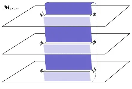
Figure 1: An artist’s impression of the Riemann surfaceMn,x1,x2 forn= 3 with field insertions
φ at the branch pointsx1,x2.
where again Zn is such that it and its derivative at n = 1 are 1 and ε is a short distance cut-off. Compared to (9) the expression (14) involves not only a different twist field but also a normalization given by hφ(x1)φ(x2)in. For CFT it is easy to interpret this normalization as
simply the norm of the ground state which in radial quantization is created by the action of the fieldφon the conformal vacuum. As for the unitary case, it is easy to show that the formula (14) when inserted in (4) reproduces (7) for CFT. It is natural to assume that the same expression will hold beyond criticality. This paper is a first step towards putting this assumption to the test beyond criticality.
2.1 Summary of main results
From the formulae above it is clear that a study of the EE in massive QFT is in principle only possible by studying correlation functions of twist fields. This approach has been pursued successfully in several works [44, 56, 45] where the ratio of partition functions (9) at large distancesr =|x1−x2|(the infrared (IR) region) has been studied for unitary 1+1-dimensional
integrable QFTs. Integrability means that in these models there is no particle production in any scattering process and that the scattering (S) matrix factorizes into products of two-particle
S-matrices which can be calculated exactly (for reviews see e.g. [57, 58, 59, 60, 61]). Although most of the integrable theories studied in this framework are unitary, well-known examples of non-unitary integrable QFTs exist. Best known among those examples is the Lee-Yang model whose exact S-matrix was first given in [62].
evaluation of (9) for various unitary models. In this paper we will pursue this program for the Lee-Yang model employing the formula (14). Our main results can be summarized as follows:
1) Form factor program for twist fields: We have found that the twist field form factor equations together with the requirement of form factor clustering are sufficient conditions to entirely fix all form factor solutions for any particle numbers. In particular, these constraints immediately give rise to two form factor families, naturally identifiable with the fieldsT and :Tφ:. We have carried out a zeroth order perturbed CFT computation of the twist field two-point function for several values ofnand compared this to a truncated form factor expansion of the same correlator. The former is expected to be accurate at short distances, the latter at large distances. Nevertheless, the agreement is relatively good, thus confirming the validity of the form factors found.
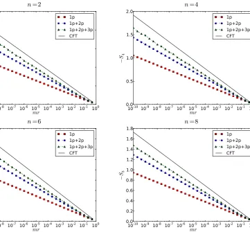
2) Saturation of the EE at large subsystem size: Let us absorb all non-universalo(1) constants of the short-distance behaviour of the R´enyi EE into a short-distance cutoffn. Subtracting this non-universal contribution, the EE at large distances then saturates to a universal constant which can be calculated using QFT. More precisely, we find
SA(n)(r) ∼ −ceff(n+ 1)
6n log(mn) +Un+o(1) (mr→ ∞)
∼ ceff(n+ 1)
6n log(r/n) +o(1) (mr→0) (15)
where the universal saturationUn is given by
Un= 1 1−n
Kφn K:Tφ:
. (16)
The constantsKO are fundamental properties of QFT fieldsO, defined by
KO =
limmr→0(mr)4xOhO(r)Oe(0)i limmr→∞hO(r)Oe(0)i
(17)
wherexO is the unique exponent making the limit finite and nonzero, and whereOe is the “conjugate” under internal symmetries (φe=φ and :^Tφ: =: ˜Tφ :). In the unitary case,
xOis the conformal dimension of O, andKO =m2∆OhOi−1 under the CFT normalization
ofO. In the non-unitary case, both of these statements are modified. In particular, in the Lee-Yang model, these constants can be expressed in terms of massive QFT and of CFT data as
Kφ=m2∆ ˜
Cφφφ
hφi, K:Tφ:=m
4∆:Tφ:−2n∆
˜
Cφ1···φn
:Tφ::Tφ:hφin
h:Tφ:i2 (18)
where the vacuum expectation values are under CFT normalization, and ˜Cφφφ and ˜Cφ1···φn
:Tφ::Tφ:
are structure constants of conformal OPEs. ConstantsKO can also be expressed solely in
3) Leading order correction to saturation: For unitary theories, one of the most interesting results [44, 56] has been the identification of a universal leading order correction to the large-distance (large-r) saturation of the entropy of all unitary integrable theories. This exponentially decaying correction, of order o(e−2mr), has a higher degree of universality than usual QFT quantities, as it only depends on the particle spectrum of the model. In [46] it was shown that, even more strikingly, this feature holds beyond integrability. This, however, seems to be broken in non-unitary models. For the Lee-Yang model, we found
SA(r)∼ − 2
15log(m) +U−aK0(mr) +O(e
−2mr), (19)
where a =−0.0769782...is a constant that is (a priori) model-dependent. This suggests that we may use this feature of the EE as a means to identify non-unitary critical points. Indeed, given a spin chain model whose critical point is not known, a study of entangle-ment at criticality will reveal the value of ceff. However, this does not say if ceff =c or
not. Considering large size corrections away from criticality will reveal different types of exponential decay depending on whether or not the theory is unitary.
3
S
-matrix and form factors in the Lee-Yang model
3.1 S-matrix
The Lee-Yang model is one of the simplest 1+1 dimensional integrable QFTs. From the CFT point of view, it may be regarded as a perturbation of the non-unitary minimal model associated with central charge c = −22
5. The primary operator content of the theory is very simple,
consisting of the identity and a scalar field φ of conformal dimension ∆ =−1
5. Perturbing this
CFT by the scalar field we obtain the massive Lee-Yang model. This theory has a single particle spectrum. The scattering amplitude corresponding to the scattering of two particles of the same type was found by Cardy and Mussardo [62] and can be written as
S(θ) = tanh
1 2 θ+
2πi
3
tanh12 θ−2πi
3
.
It has a pole in the physical sheet at θ= 2πi3 corresponding to the formation of a bound state, which in this case is the same fundamental particle of the theory. We note that the non-unitarity is manifested by the fact that the associated residue has the wrong sign. Nevertheless, the corresponding integrable massive model is well defined. The n-copy model, where the Zn twist fields live, possesses n particle speciesµ = 1, . . . , n, and a two-particle scattering matrix given by Sµ1µ2(θ) =S(θ)
δµ1,µ2.
3.2 Form factor expansions of two-point functions
In this paper we study the correlators hT(r) ˜T(0)i and, especially, h: Tφ : (r) : ˜Tφ : (0)i and
matrix elements of these operators. The matrix elements of relevance, also known as form factors, are defined as
FO|µ1...µk
k (θ1, . . . , θk) :=h0|O(0)|θ1, . . . , θki
in
µ1,...,µk , (20)
for a local field O. Here |0i represents the vacuum state and|θ1, . . . , θkiinµ1,...,µk are the physical
“in” asymptotic states of massive QFT. They carry indices µi, which are quantum numbers characterizing the various particle species, and depend on the real parameters θi, which are called rapidities. The energy and momentum of a particle of mass mi are expressed in terms of its rapidity θi as micoshθi and misinhθi, respectively. In terms of form factors, two-point correlation functions (in unitary models) may be expanded as
hO(r)O†(0)i=
∞ X k=0 1 k! n X
µ1,...,µk=1
k Y j=1 ∞ Z −∞ dθj (2π)
F
O|µ1...µk
k (θ1, . . . , θk) 2 e −rm k P j=1
coshθj
. (21)
As mentioned, the Lee-Yang model is non-unitary. As was noted in [65, 66], non-unitarity affects the form factor expansion. A consequence of this is that many fields appear to be non-Hermitian under the Hilbert structure of asymptotic states. In the Lee-Yang model, an exact cal-culation of the form factors of the fieldφshows that h0|φ(0)|θ1, . . . , θkiin
∗
6
=inhθ1, . . . , θk|φ(0)|0i, where the right-hand side can be obtained by crossing symmetry. However, it turns out that the relation is surprisingly simple:
hφi−1h0|φ(0)|θ1, . . . , θkiin ∗
= (−1)khφi−1 inhθ1, . . . , θk|φ(0)|0i. (22) As a consequence, the form factor expansion of the two-point function of the fieldφ, normalized by the square of the VEV, is a modification of (21) where sign factors (−1)k are included for the terms involving thek-particle form factors. This gives rise, in the single-copy Lee-Yang model, to:
hφ(r)φ(0)i
hφi2 =
∞
X
k=0
(−1)k
k! k Y j=1 ∞ Z −∞ dθj (2π)
hφi
−1Fφ
k(θ1, . . . , θk) 2 e −rm k P j=1
coshθj
. (23)
A natural way to understand this modification is through a discussion of the bound-state singularity occurring in the form factors. The additional (−1)k guarantees that the bound-state residue of the analytic continuation of the k-particle integrand, which, like that of the scattering matrix, has the wrong sign, is related to the k−1-particle integrand in a way that would guarantee locality properties. As we will see below, form factors of twist fields : Tφ :, : ˜Tφ:,T and ˜T are subject to similar bound-state residue equations as those ofφ. Hence, this interpretation suggests that a similar modification of (21) occurs for the form factor expansion of h:Tφ: (r) : ˜Tφ: (0) and of hT(r) ˜T(0)i. That is, in then-copy model,
hO(r) ˜O(0)i
hOi2 =
∞
X
k=0
(−1)k
k!
n X
µ1,...,µk=1
k Y j=1 ∞ Z −∞ dθj (2π)
hOi
−1FO|µ1...µk
k (θ1, . . . , θk) 2 e −rm k P j=1
coshθj
for both O = T, ˜O = ˜T and O =: Tφ :, ˜O =: ˜Tφ :. Here we have used the fact that by symmetry under inversion of copies, hT i˜ = hT i and h: ˜Tφ :i = h: Tφ :i, and the form factor expansion includes sums over the copy numbers µj. That this is the correct expansion follows from an equation similar to (22) for twist fields, see subsection 4.4
Finally, since the fieldφ is no longer Hermitian, its VEV is no longer expected to be real. As was shown by Zamolodchikov,hφi is in fact purely imaginary – this can be explained by the fact that it occurs in the formal massive Lee-Yang action (written as a perturbation of the CFT action) with a purely imaginary coupling constant. A similar phenomenon makes the VEVs
hT i and h: Tφ :i not necessarily real. We will determine their phases (up to multiples of π) by evaluating analytically the normalization of their leading short-distance power-law, and by observing numerically that the right-hand side of (24) is positive for all mr.
3.3 Short-distance behaviour from form factors
Form factor expansions (21) and (23) are naturally large-distance expansions, in that they converge very rapidly for large values of rm. However, in many cases we want to explore small values of rm. In such cases two-point functions generally develop power-law behaviours inrm
and it is very difficult to extract the precise power from a form factor expansion such as those above.
It was realized a long time ago [65] (see also [67] for a nice derivation and application to various models and [68] for a generalization to boundary theories) that if one is interested in the short-distance behaviour of correlators then an expansion of the logarithm of two-point function is more appropriate:
log hO(r) ˜O(0)i
hOi2
! =
∞
X
k=1
(−1)k
k!
n X
µ1,...,µk=1
k Y
j=1
∞
Z
−∞
dθj (2π)
H
O|µ1,...,µk
k (θ1,· · · , θk)e
−rm
k P j=1
coshθj
.(25)
The functions HO|µ1,...,µk
k (θ1,· · · , θn) must of course be chosen so that the expansion (21) is
recovered when exponentiating (25). This condition automatically implies for example that
HO|µ1
1 (θ) = hOi
−2|FO|µ1 1 (θ)|
2, (26)
HO|µ1µ2
2 (θ1, θ2) = hOi−2|F
O|µ1µ2
2 (θ1, θ2)|2−H
O|µ1 1 (θ1)H
O|µ2
1 (θ2), (27) HO|µ1µ2µ3
3 (θ1, θ2, θ3) = hOi−2|F
O|µ1µ2µ3
3 (θ1, θ2, θ3)|2−H
O|µ1 1 (θ1)H
O|µ2 1 (θ2)H
O|µ3 1 (θ3)
−HO|µ1µ2
2 (θ1, θ2)H
O|µ3
1 (θ3)−H
O|µ2µ3
2 (θ2, θ3)H
O|µ1 1 (θ1)
−HO|µ1µ3
2 (θ1, θ3)H
O|µ2
1 (θ2). (28)
In general the Hk functions can be interpreted as the “connected parts” of the Fk functions (they are “cumulants” with respect to the rapidities). These are such that, if the clustering decomposition holds for the Fk’s at large rapidities for all k, that is
lim θ1,...,θk→∞
FO|µ1...µk+`
k+` (θ1, . . . , θk+`) =
FO|µ1...µk
k (θ1, . . . , θk)F
O|µk+1...µk+`
` (θk+1, . . . , θk+`)
∀k, `∈N, then the Hk’s vanish at large rapidities for all k.
Thanks to this vanishing, formr 1 we now expect each summand in the sum over k in the expression above to be dominated by a leading term proportional to log(mr). The constant coefficient of this term, summed over all particle contributions, will then give the power which governs the short-distance behaviour of the two point function. Let us call this power −4xO.
Then, carrying out one integral in (25) and expanding the result for smallmrwe find [65, 67, 68]
xO =
1 4π
∞
X
k=0
(−1)k
k!
n X
µ1,...,µk=1
k Y
j=2
∞
Z
−∞
dθj (2π)
H
O|µ1,...,µk
k (0, θ2,· · · , θk). (30)
This was used for the fieldφin [66] and shown to agree well with conformal field theory results. In addition, the proportionality constant (17) of the power law behaviour at short distances,
hO(r) ˜O(0)i
hOi2 ∼KO(mr)
−4xO (mr→0) (31)
can also be extracted from the form factor expansion. It was shown in [67] that by considering the leading correction to the log(mr) term in (25) one may also find a form factor expansion for the constantKO which is given by:
KO= exp
− 1
π
∞
X
k=0
(−1)k
k!
n X
µ1,...,µk=1
k Y
j=2
∞
Z
−∞
dθj (2π)
H
O|µ1,...,µk
k (0, θ2,· · ·, θk)(ln
ξ
2 +γ)
, (32)
with ξ2 =
Pk
j=2coshθi+ 1 2
−Pkj=2sinhθi
2
and where γ = 0.5772157... is the
Euler-Mascheroni constant.
4
Twist field form factors
4.1 Form factor equations and minimal form factors
In what follows we will considerk-particle form factorsFO|µ1···µk(θ
1, θ2, . . . , θk) for a generic twist field O. We will later identify this field with T or :Tφ: depending on various properties of the form factor solutions we obtain.
The two-particle form factor must satisfy (in the two-particle case we use the single argument
θ=θ1−θ2)
FO|11(θ) =S(θ)FO|11(−θ) =FO|11(−θ+ 2πin), (33)
and the kinematic residue equations
Res
θ= 0
F2O|µµ¯ (θ+iπ) = ihOi, (34)
Res
θ= 0
F2O|µ¯µˆ(θ+iπ) = −ihOi. (35)
Here and below we use ˆµ=µ−1 modn. Higher particle versions of these equations read
Res ¯
θ0=θ0
FO|µµµ¯ 1...µk
k+2 (¯θ0+iπ, θ0, θ1. . . , θk) = i F
O|µ1...µk
k (θ1, . . . , θk), (36)
Res ¯
θ0=θ0
FO|µ¯µµˆ 1...µk
k+2 (¯θ0+iπ, θ0, θ1. . . , θk) = −i k Y
i=1 Sµµ(ˆn)
i(θ0i)F
O|µ1...µk
k (θ1, . . . , θk). (37) For this model there is the added difficulty of having to solve also the bound state residue equation associated to the scattering processa+a→awhereais the Lee-Yang particle on copy
a. This takes the form
Res
θ= ¯θ
FO|aaµ1...µn−1
n+1 (θ+ iπ
3 ,θ¯−
iπ
3, θ1, . . . , θn−1) =iΓF
O|aµ1...µn−1
n (θ, θ1, . . . , θn−1) (38)
where the so-called three-point coupling is fixed by
Γ2 =−i lim θ→2πi
3
(θ−2πi
3 )S(θ) =−2
√
3 (39)
and by choosing the negative imaginary direction: Γ =−i21/231/4. Forn= 1 this equation fixes the one particle form factor (which for spinless fields must be rapidity independent) through the equation
Res
θ= ¯θ
F2O|aa(θ−θ¯+2iπ
3 ) =iΓF
O|a
1 . (40)
minimal form factor. A minimal form factor is a solution of (33) which has no poles in the (extended) physical sheet θ ∈ [0,2πn) except possibly for bound state poles, and which tends to unity as |θ| → ∞. It turns out that this particular Riemann-Hilbert problem has a unique solution, and this solution possesses bound state poles with nonzero residues:
Fmin(θ) =a(θ, n)f(θ, n), (41)
where a(θ, n) encodes the bound state pole
a(θ, n) = cosh θ n−1
coshnθ −cos23πn, (42) and f(θ) is given by the integral representation
f(θ, n) = exp
2 Z ∞
0
sinht3sinh6t
tsinh(nt) cosh2t cosht
n+iθ
π
. (43)
The latter function admits also a representation as an infinite product of gamma functions which was already given in [44] for the sinh-Gordon model (it suffices to take B = 2/3 and to invert the formula).
The expression (43) may be obtained as a solution to (33) using a similar integral representa-tion of the two-particle scattering amplitude. In the absence of bound state poles, the resulting
f(θ, n) would directly be the minimal two-particle form factor. In the present case, however, the function tends to 1 as |θ| → ∞ but has a simple pole at θ = 0. The factor a(θ, n) is the unique one that shifts this pole towards the position of the allowed bound-state singularity in the physical sheet, without affecting the large-|θ|behaviour.
Using the integral or Gamma-function representation, it may be shown that
f(iπ, n)
f(2πi3 , n)2 = n
√
3
sin3 3πn
sin6πnsin2πn. (44) In order to compute higher particle form factors the following more general identities are im-portant
Fmin(θ+ iπ
3 )Fmin(θ−
iπ
3) =
coshθn−cos23πn
coshnθ −cosπn Fmin(θ), (45)
Fmin(θ+iπ)Fmin(θ) =
sinh2θnsinh 2θn+2iπn sinh 2θn−3iπn
sinh 2θn+56iπn. (46)
4.2 Twist field one- and two-particle form factors
the position of the field. With these conditions, the most general form the two-particle form factor can take is
F2O|11(θ) = hOisin π n
2nsinh iπ2−nθ
sinh iπ2+nθ
Fmin(θ) Fmin(iπ)
+κFmin(θ), (47)
where the first term is of the form required to solve the kinematic residue equation (and of the same form as for other theories previously studied [44]) and the second term is what is commonly termed a “kernel” solution of the kinematic residue equation (that is a solution without kinematic poles).
In generalκ is an arbitrary constant, but it may be fixed by imposing the cluster decompo-sition property, namely
lim θ→∞F
O|11
2 (θ) =κ:=
(F1O|1)2
hOi , (48)
where we have used the fact that limθ→∞Fmin11 (θ) = 1. Then, the one-particle form factor on
copy a may be fixed by combining this with equation (40), which translates into the following quadratic equation forF1O|1
F1O|1 =−1
Γ tan3πn tan2πn
f(2πi3 , n)
f(iπ, n)hOi+
(F1O|1)2
hOi
n
Γtan π
3n
f(2πi
3 , n). (49)
This leads to two possible solutions:
F1O|1 =−hOiΓcos π
3n
±2 sin2 6πn 2nsin 3πn
f(23πi, n) , (50)
where we have used the identity (44).
The presence of two solutions immediately suggests the existence of two different least-singular twist fields, by contrast to other models studied in the past. It is natural to conjecture that these are T and : Tφ :, and given this, it is a simple matter to identify their respective form factor solutions. Indeed, the former specializes to the identity at n= 1, and the latter, to
φ. We note that the solution with the negative sign specializes to 0 atn= 1, and that that with the positive sign specializes to the one-particle form factor of the field φ
F1φ F0φ =
i21/2 31/4f(2πi
3 ,1)
with F0φ=hφi= 5im
−25
24h√3 and h= 0.09704845636... (51)
found in [66] (note that the constant v(0) in [66] is v(0) = f(iπ,1)1/2 =
√
3 2 f(
2πi
3 ,1) with our
present notation, and that the coupling h was computed in [71]). These properties suggest the identifications
F1T |1
hT i =−Γ
2 cos 3πn−1 2nsin 3πn
f(2πi3 , n),
F1:Tφ:|1
h:Tφ:i =−
Γ 2nsin 3πn
4.3 Higher particle form factors
Let us now consider only form factors of the form FkO|11...1(x1, . . . , xk) := FkO(x1, . . . , xk), that is form factors involving only one particle type. This is sufficient as form factors involving other particles may be obtained from these by using the twist field form factor equations [44].
The higher particle form factors may be obtained by making the ansatz
FkO(x1, . . . , xk) =Qk(x1, ..., xk)
k Y
i<j
Fmin(θi−θj) (xi−αxj)(xj−αxi)
, (53)
where xi =eθi/n and α=eiπ/n. The functionsQk(x1, ..., xk) are symmetric in all variables and have no poles on the physical sheet.
This ansatz, as usual in the context of the computation of form factors of local fields (see e.g. [66, 72]), expresses the form factors in such a way as to explicitly separate the part containing the poles from the part which has no singularities. In addition, the explicit presence of the minimal form factor and the symmetry in the variables xi automatically gives form factors which exhibit the correct monodromy properties in the rapidities. In the context of twist fields, this ansatz was used for the first time in [69].
4.3.1 Kinematic and bound state residue equations
Using (46), the kinematic residue equation with the ansatz (53) can be rewritten as (k≥0):
Qk+2(αx0, x0, x1, . . . , xk) =x20Pk(x0, x1, . . . , xk)Qk(x1, . . . , xk), (54) where Pk is the polynomial
Pk(x0, x1, . . . , xk) =Ck(n)
k Y
b=1
(xb−α2x0)(xb−α−1x0)(xb−βx0)(xb−αβ−1x0)
, (55)
where β=e−23πin and
Ck(n) = 2 sin π n
nFmin(iπ)
α2(k+1) =C0(n)α2k. (56)
Denoting σi(k) the i-th elementary symmetric polynomial on k variables x1, . . . , xk, which can be defined by means of the generating function,
k X
i=0
xk−iσi(k)= k Y
i=1
(xi+x), (57)
we can rewrite Pk(x0, x1, . . . , xk) as
Ck(n) k X
a,b,c,d=0
(−α2x0)k−a(−α−1x0)k−b(−αβ−1x0)k−c(−βx0)k−dσa(k)σ
(k)
b σ
(k)
c σ
(k)
In the following we will omit the upper index(k) when there is no confusion possible.
Besides (54), another equation that arises from the ansatz (53) is that using the bound state residue equation (38). The simplest case of this equation was given in (40) and this allowed us, in combination with the clustering property, to fix the one-particle form factor (49). For higher particles, using (45) we find (k≥1)
Qk+1(x0β− 1 2, x0β
1
2, x1, . . . , xk−1) =x2
0Uk(x0, x1, . . . , xk−1)Qk(x0, x1, . . . , xk−1), (59)
with
Uk(x0, x1, . . . , xk−1) = Hk(n) k−1
Y
i=1
(xi−β−2x0)(xi−β2x0) (60)
= Hk(n) k−1
X
a,b=0
(−β−2x0)k−1−a(−β2x0)k−1−bσa(k−1)σ
(k−1)
b , and
Hk(n) =
4Γ sin2 2πn
ntan 3πna(iπ)f(2πi3 )(−α) k =H
1(n)(−α)k−1. (61)
From the ansatz (53) it follows that Q1=F
O|1 1 .
4.3.2 Three-particle form factors
First let us analyze the two-particle case. We have by definition that F0O = Q0 = hOi, and
comparing to (47), we obtain the polynomial
Q2(x1, x2) =hOiC0(n)α−1σ2+
(F1O|1)2
hOi (1 +α)
2σ
2−ασ21
. (62)
It is a simple matter to verify that this is indeed in agreement with the kinematic residue equation (54); given Q0 this is the most general solution to (54) (k = 0), as was shown in
[69] (in particular, the second term vanishes at x1 = αx2). Further, replacing (F
O|1
1 )2/hOi by
the linear combination of the zero- and one-particle form factors, Q0 and Q1(x1), occurring via
the quadratic equation (49), one can check that (62) is in agreement with (59). In fact, given arbitraryQ0 andQ1(x1), the resulting expression is theuniquesolution to (54) (k= 0) and (59)
(k= 1).
As was shown above, the additional condition of clustering imposes the one-particle form factor to take only two possible values (proportional to the vacuum expectation value), according to (52). For n = 1 the solution (62) is either zero (if we take the first solution in (52)) or it reduces to Zamolodchikov’s two particle solution for the Lee-Yang field [66] (if we take instead the second solution in (52)). This is in accordance with identifying the two-particle form factors with those of T and :Tφ:, respectively.
Interestingly, it turns out that the above structure subsists to higher particles: givenQ2(x1, x2)
(k = 1) and (59) (k = 2) for the polynomial Q3(x1, x2, x3). The solution has the following
structure:
Q3(x1, x2, x3) =A1σ13σ3+A2σ12σ22+A3σ1σ2σ3+A4σ23+A5σ23, (63)
where the parametersAi are complicated functions ofnbut rapidity-independent. The detailed computation of Q3(x1, x2, x3) and the values of Ai are reported in appendix C, and note in particular that the polynomialsσ61 and σ14σ2 have vanishing coefficients.
Again it is interesting to consider the limit n → 1 of the functions Ai above. Using the two solutions (52), we now note that all constants vanish, Ai = 0, when we consider that corresponding to the operator T (whereF1T |1 = 0 forn= 1), thus the three particle form factor also vanishes. On the other hand, if we consider the other solution in (52), which at n = 1 should correspond to the field φ, we find
A1 =A4 =A5 = 0, A2 =−A3 =
(F1φ)2H1(1)
hφi =
iπm231/4
27/2f(iπ,1)3/2, (64)
and a simple computation shows that our three-particle form factor, as expected, reduces to Zamolodchikov’s solution [66].
It is tempting to use this benchmark (agreement with Zamolodchikov’s solutions) to try and find the general solution for higher particle numbers. However, as the three-particle case shows, the reduction to n= 1 occurs thanks to great simplifications. At this stage, it is unfortunately not obvious at all how high-particle solutions may be constructed other than by brute force computation. The main reason for this is the presence of two (rather than one) kinematic pole in the form factor ansatz (53). This leads to polynomials QOk(x1, . . . , xk) of much higher degree than is the case in the standard form factor program.
Despite the complexity of the expression (162), there are certain simplifications that can be used to rewrite the three-particle form factor in a form which is more suitable for numerical computations. It turns out that
F3O|111(θ1, θ2, θ3) = f3(x1, ..., xk)
3
Y
i<j
Fmin(θi−θj) (xi−αxj)(xj−αxi)
−(F
O|1
1 )2hOi−1H1(n)
4αsin 6πnsin 56πn
3
Y
i<j
Fmin(θi−θj), (65) where f3(θ1, θ2, θ3) is the function that is obtained from Q3(θ1, θ2, θ3) in (162) by setting all
terms proportional tohOi−1 to zero. In other words, when divided byQ
i<j(xi−αxj)(xj−αxi), all those terms simplify giving just the second summand in the formula above. This summand represents a kernel solution to the form factor equations, in the sense already described in subsection 3.2.
Finally, note that
lim θ1→∞
F3O|111(θ1, θ2, θ3) =
α−1F1O|1C0(n)
4 sin 6πn
sin 56πn
4 cos2 3πnx2x3−(x2+x3)2
Fmin(θ2−θ3)
(x2−αx3)(x3−αx2)
−(F
O|1
1 )2hOi−1H1(n)
4αsin 6πn
sin 56πnFmin(θ2−θ3) =
F1O|1F2O|11(θ2−θ3)
where we have used the property
F1O|1H1(n) =hOiα−1C0(n)−4αhOi−1(F
O|1 1 )2sin
π 6n
sin
5π
6n
, (67)
which can easily be derived from (49), (56) and (61). In other words, the three-particle solution automatically satisfies the clustering property. This is an extremely nontrivial check of the validity of the three-particle solution. This situation is in contrast to that of the sinh-Gordon model [69], where at each particle number, the clustering property has to be imposed in order to uniquely fix the solution. It also follows from the result above and the cluster property of the two-particle form factor that
lim θ1,θ2→∞
F3O|111(θ1, θ2, θ3) =
(F1O|1)3
hOi2 . (68)
Properties (66) and (68) are very important as they insure the convergence of the integrals (25) fork= 3.
4.4 Form factors of the fields T˜ and : ˜Tφ:
In the previous subsections we have concentrated our analysis on computing the form factors of the fields T and : Tφ:. However, the correlators we are interested in also involve the fields ˜T
and : ˜Tφ: thus their form factors are also required. In fact the form factors of all these fields are not independent from each other. We may think of T and :Tφ: and of ˜T and : ˜Tφ : as twist fields associated to the two opposite cyclic permutation symmetriesi7→i+ 1 andi+ 17→i
(i= 1, . . . , n, n+ 1≡1). From the additional symmetry under the inversion of copy numbers it follows that
FT |µ1...µk
k (θ1,· · · , θk) =F
˜
T |(n−µ1)...(n−µk)
k (θ1,· · · , θk), (69)
and similarly for : Tφ : and : ˜Tφ :. At the same time, as already explained in subsection 3.2, from the non-unitarity of the theory we would expect that
h
hT i−1FT |µ1...µk
k (θ1,· · ·, θk)
i∗
= (−1)khT i−1FT |˜µ1...µk
k (θk,· · ·, θ1)
= (−1)khT i−1FT |(n−µ1)...(n−µk)
k (θk,· · ·, θ1) (70)
(note that hT i = hT i˜ ). These equations both define the form factors of ˜T and impose the condition expressed by the last equality above on the form factors of T. We have verified that this is satisfied for all our solutions, and that similar equations hold for :Tφ:. These equations are the counter-part of (22) for twist fields, and show that the form factor expansion (24) is correct.
Finally, another important relation which we have used in subsequent computations is the following identity
FT |µ1...µk
k (θ1,· · · , θk) =F
T |1...1
k (θ1+ 2πi(µ1−1),· · · , θk+ 2πi(µk−1)) µ1 < . . . < µk, (71)
5
Identification of twist field operators: numerical results
In previous sections we have provided compelling evidence for the identification of the two families of form factor solutions that we have obtained with the twist fieldsT and :Tφ:. This evidence is based on the (highly non-trivial) fact that the one-particle and higher form factors of the field we identified asT vanish atn= 1 whereas those of :Tφ: reduce to the form factors of φ obtained in [66]. Further evidence may be gathered by, for example, examining the short distance behaviour of the correlators hT(r) ˜T(0)i and h:Tφ: (r) : ˜Tφ: (0)i. We must therefore first understand what the expected behaviour of such correlators should be for the theory at hand.
Let us first consider the conformal field theory. In CFT such correlators are expected to
converge at small distances as
hT(r) ˜T(0)iCFT=r−4∆T, (72)
and
h:Tφ: (r) : ˜Tφ: (0)iCFT=r−4∆:Tφ:. (73)
Indeed note that the powers above are positive for the Lee-Yang model as both c and ∆ are negative (see section 3). This is of course a consequence of non-unitarity.
In the massive theory, however, we expect that the leading short distance behaviours of these correlators should be described by a different power law:
hT(r) ˜T(0)i ∝r−4∆T+2n∆, (74)
and
h:Tφ: (r) : ˜Tφ: (0)i ∝r−4∆:Tφ:+2n∆. (75)
The reason for this is entirely analogous to the observation made in [66] regarding the correlator hφ(r)φ(0)i. It was found that for short distance in the massive theory the leading behaviour of this correlator wasr−2∆rather than the conformal behaviourr−4∆. Zamolodchikov argued that this was due to the fact that the leading behaviour of the conformal OPE comes from the field φ rather than the identity. In the massive theory the expectation valuehφi 6= 0 and therefore the contribution to the OPE from the field φitself becomes the dominating term in the short distance expansion of the two-point function.
Similarly, it is possible to argue that the leading contribution to the OPEs ofT and ˜T and of :Tφ: and : ˜Tφ: corresponds to the fieldφ1φ2. . . φnwhereφi represents the fieldφon copyi. This field has dimension n∆, and it is the field of smallest (most negative) conformal dimension that can be constructed in the n-copy Lee-Yang model. Since its expectation value is nonzero, it thus gives the leading contribution at short distances. Massive OPEs of twist fields will be discussed in more detail in section 6.
Thus, by employing a form factor expansion we may check whether the expected behaviours are indeed recovered from our form factor solutions. We will include up to three particle form factors as done in [66]. We have performed a numerical evaluation of the formula (30) including up to three particle form factors for the twist fieldsT and :Tφ:. We confirm with good accuracy that the twist fields exhibit the behaviours (74) and (75) for mr 1. This means that (30) holds with xT = ∆T −n∆/2 and x:Tφ:= ∆:Tφ:−n∆/2. The tables and plots below show our
n 2 3 4 5 8 10 CFT (−4xT) 103 = 0.3 3445 = 0.756 2320 = 1.15 3825 = 1.52 10340 = 2.575 16350 = 3.26
[image:22.595.78.528.94.166.2]1-particle 0.209643 0.442562 0.656773 0.861066 1.44896 1.83206 1+2-particles 0.259028 0.564549 0.842992 1.10754 1.86697 2.3611 1+2+3-particles 0.279487 0.625075 0.937636 1.23376 2.13554 2.70666
Table 1: Study of the two-point function hT(r) ˜T(0)i of the n-copy Lee-Yang theory at short distances. Near the critical point we expect this correlator to exhibit a power-law behaviour of the formr−4xT wherex
T = ∆T −n2∆ =−12n +6011n. This value should be best reproduced in the
massive theory the more form factor contributions are added. The data above show that this expectation is indeed met by considering up to three-particle form factors.
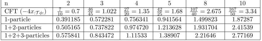
n 2 3 4 5 8 10
CFT (−4x:Tφ:) 107 = 0.7 4645 = 1.022 2720 = 1.35 4225 = 1.68 10740 = 2.675 16750 = 3.34
1-particle 0.391185 0.572281 0.756341 0.941564 1.499823 1.87287 1+2-particles 0.505165 0.737822 0.974720 1.213628 1.931704 2.41539 1+2+3-particles 0.575841 0.843472 1.11533 1.38907 2.21646 2.77169
Table 2: Study of the two-point function h:Tφ: (r) : ˜Tφ: (0)i of then-copy Lee-Yang theory at short distances. Near the critical point we expect this correlator to exhibit a power-law behaviour of the form r−4x:Tφ: where x
:Tφ: = ∆:Tφ:− n2∆ =−12n − 601n. The data above show
good agreement with CFT by considering up to three-particle form factors.
6
Comparison with perturbed conformal field theory results
A further consistency check of our form factor solutions may be carried out by comparing a form factor expansion of the correlatorshT(x1) ˜T(x2)i andh:Tφ: (x1) : ˜Tφ: (x2)ito its counterpart
in perturbed conformal field theory.
6.1 Conformal perturbation theory and twist fields structure constants
We may regard the action of the integrable quantum field theory as a perturbation of Lee-Yang CFT action by a term proportional to a coupling constantλand the CFT field φ(x,x¯) of conformal dimension ∆,
SIQF T =SCF T +iλ Z
d2x φ(x,x¯), (76)
[image:22.595.78.528.267.338.2]2 3 4 5 n6 7 8 9 10 0.0
0.5 1.0 1.5 2.0 2.5 3.0 3.5 4.0
−
4
xT
1p 1p+2p 1p+2p+3p CFT
2 3 4 5 6 n 7 8 9 10 11
0.0 0.5 1.0 1.5 2.0 2.5 3.0 3.5 4.0
−
4
x:Tφ
:
[image:23.595.87.530.100.263.2]1p 1p+2p 1p+2p+3p CFT
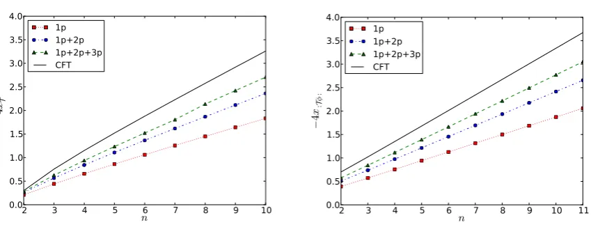
Figure 2: Graphical representation of −4xT and −4x:Tφ: for n≤11. The squares, circles and
triangles, represent the up to one-, two- and three-particle form factor contributions. The black solid line represents the exact values at criticality. All curves clearly show strong linearity in n
which is consistent with the CFT behaviour, where the coefficient of n(e.g. slope of the curves) approaches the CFT value as more form factor contributions are added. The agreement with CFT gets worse as n increases. This is also to be expected as the larger n is, the larger the contribution of higher particle form factors becomes (all form factor contributions are in fact proportional ton).
λ, are nonzero. The same type of comparison between a form factor and a perturbed CFT computation was carried out in [66] for the two-point function of the field φin Lee-Yang.
Let us now consider the OPEs of T with ˜T and of : Tφ : with : ˜Tφ :. They involve only fields in the non-twisted sector (we mean by this all fields constructed by considering
n non-interacting copies of the fields of the original theory) and by construction they must be invariant under cyclic permutation of the copies. Let us consider the following primary, cyclically invariant, homogeneous fields, composed of multilinears in the fields φi on the various copies: we label them by sets {k1, . . . , kJ} of J different integers in [1, n] for J = 1,2, . . . , n (we may
take k1 <· · ·< kJ), and take them to be
Φk1,...,kJ :=
φk1· · ·φkJ + cyclic permutations
Sk1,...,kJ
. (77)
The symmetry factor Sk1,...,kJ is equal to the order of the subgroup of the cyclic replica permu-tations which preserve the sequencek1, k2, . . . , kJ of replica indices. That is, Φk1,...,kJ is the sum,
over all elements σ ∈ Zn in the cyclic replica permutation group Zn, of σ(φk1· · ·φkJ), divided
by the order of the stabilizer, in Zn, of φk1· · ·φkJ. This definition guarantees that in Φk1,...,kJ,
every independent multilinear term, including the initial term φk1· · ·φkJ itself, appears with
factors for low values of J can be written explicitly:
S1,k =
2 (neven, k=n/2 + 1) 1 (otherwise)
S1,k,j =
3 (k−1 =j−k=n+ 1−j) 1 (otherwise).
S1,k,j,p =
4 (k−1 =j−k=p−j=n+ 1−p) 2 (k−1 =p−j=6 j−k=n+ 1−p) 1 (otherwise)
(78)
The fields Φk1,...,kJ have conformal dimensions J∆. In order to have a basis of primary,
cyclically invariant homogeneous fields of dimension J∆, we need to further restrict the indices
k1, . . . , kJ. We may certainly fix k1 = 1, and further restrictions hold due to the residual
equivalence relation generated by{1, . . . , kJ} ∼ {1, n+2−kJ, n+1+k2−kJ, . . . , n+1+kJ−1−kJ}. More generally, in the set of all replica-index sets {k1, . . . , kJ}, there is a foliation byZn orbits, and a basis of fields Φk1,...,kJ can be taken as fields parametrised by single representatives of
each Zn orbit.
Let us give simple examples. For J = 1, we have Φ1 =
Pn
j=1φj. For J = 2 the basis is Φ1,2 =φ1φ2 + alln−1 cyclic permutations, Φ1,3 =φ1φ3 + all n−1 cyclic permutations, etc.
until Φ1,[n/2]+1 = φ1φ[n/2]+1 + all n−1 cyclic permutations (if n is odd), or until Φ1,n/2+1 = φ1φn/2+1 + all cyclic permutations up to φn/2φn (if n is even). In particular for n = 3, we have φ1φ2+φ2φ3+φ3φ1 only; forn= 4, we haveφ1φ2+φ2φ3+φ3φ4+φ4φ1 andφ1φ3+φ2φ4;
etc. There is a unique field at J = n: Φ1,...,n = φ1φ2. . . φn, which has dimension n∆. As
mentioned, this field is very important in non-unitary models since for ∆ < 0 it provides the leading contribution (for small r) to the OPE, as it is the field of lowest conformal dimension.
The OPEs in the massive theory can be regarded as “deformations” of the conformal OPEs such that the structure constants are replaced by functions of mr. Denoting by O and ˜O any given pair of conjugate (i.e. whose twist actions cancel out) twist fields, it takes the form
O(x1) ˜O(x2) ∼ r−4∆O
CO1O˜(mr)1+CΦ1
OO˜(mr)r
2∆Φ 1(x2)
+
[n/2]+1
X
k=2 CΦ1,k
OO˜ (mr)r
4∆Φ
1,k(x2) +. . .+C Φ1,...,n
OO˜ (mr)r
2n∆Φ
1,...,n(x2)
+Virasoro descendants, (79)
where r:=|x1−x2|,m is the physical mass of the Lee-Yang model. The functions
CΦk1,...,kp
OO˜ (mr) = ˜C
Φk1,...,kp
OO˜
1 +CΦk1,...,kp 1 (mr)
2−2∆+CΦk1,...,kp
2 (mr)
2(2−2∆)+· · ·, (80)
admit an expansion in integer powers of the coupling λ, hence in powers of (mr)2−2∆, and the
constants ˜CΦk1,...,kp
OO˜ are the structure constants of the CFT. In our analysis we will in fact only
through the non-vanishing expectation values of OPE fields. The analysis is still non-trivial because of the presence of nonzero expectation values. Note that with the definition (11) and the standard definition of T and ˜T we have the conformal normalization
˜
CT1T˜ = ˜C:1Tφ:: ˜Tφ:= 1. (81)
The conformal OPEs (and structure constants) of the branch point twist fieldT have been studied in several places in the literature. The most general study can be found in Appendix A of [74] where general formulae for the structure constants associated to the OPE ofT with ˜T in general (unitary) CFT are given. Structure constants have also played an important role within the study of the entanglement of disconnected regions [75, 76]. More recently the structure constants of other types of twist fields which arise naturally within the study of the negativity have been studied in [77, 78]. However we do not know of any studies of the OPE and structure constants of composite fields such as :Tφ:. Here we provide explicit step-by-step computations of the conformal structure constants ˜CTΦ1T˜, ˜CΦ1
:Tφ:: ˜Tφ:, ˜C Φ1,k
TT˜ , ˜C Φ1,k
:Tφ:: ˜Tφ:, ˜C Φ1,k,j
TT˜ and ˜C Φ1,k,j,p
TT˜ (see
appendix D for details) which are proportional to one-, two-, three- and four-point functions of the field φ(other structure constants would involve higher-point functions, which are harder to access). Our computations focus on the Lee-Yang model but could be easily generalized to other minimal models (for the fieldT the ingredients needed for such generalization are already provided in [74]). Other structure constants and massive corrections thereof will involve higher point functions. The results are:
˜
CTΦ1T˜ = 0, C˜Φ1,k
TT˜ =n
−4∆|1−e2πi(nk−1)|−4∆ for k >1,
˜
CΦ1,k,j
TT˜ = n
−6∆C˜φ
φφ|(1−e
2πi(k−1)
n )(1−e
2πi(j−1)
n )(1−e
2πi(j−k)
n )|−2∆ for j > k >1,
˜
CTΦ1T˜,k,j,p = n−8∆hφ(e2nπi)φ(e
2πik n )φ(e
2πij n )φ(e
2πip
n )i for p > j > k >1,
˜
CΦ1
:Tφ:: ˜Tφ: = n
−2∆C˜φ φφ, C˜
Φ1,k
:Tφ:: ˜Tφ:=n
−4∆κ1−e2πi(nk−1) for k >1, (82)
where κ is a model-dependent function which characterizes the four-point function of fieldsφ
hφ(x1)φ(x2)φ(x3)φ(x4)i=κ(η)|x1−x4|−4∆|x2−x3|−4∆, η =
x12x34 x13x24
. (83)
Other structure constants may be computed in terms of higher-point functions so that in general we expect
˜
CΦ1,k2,...,kJ
TT˜ =n
−2J∆hφ(e2πi n )φ(e
2πik2
n ). . . φ(e
2πikJ
n )i, (84)
and
˜
CΦ1,k2,...,kJ :Tφ:: ˜Tφ: =n
−2J∆κ(e2πik2
n , . . . , e
2πikJ
n ), (85)
with
κ(x1, x2, . . .) = lim
y→∞|y|
4∆hφ(0)φ(1)φ(y)φ(x
1)φ(x2)· · ·i. (86)
The difficulty of calculating such terms is then reduced to the difficulty of obtaining higher-point functions in CFT. Such higher-higher-point functions will also be required in order to obtain most massive corrections to the CFT structure constants, a problem which we will not be addressing in this work.
6.2 The case n = 2
As explained earlier, obtaining the CFT structure constants becomes a difficult problem for the field :Tφ: as soon as we consider OPE terms involving products of more than two fields and for the field T when we consider products involving more than four fields. For this reason, the casen= 2 is particularly interesting as in this case the leading contribution to the OPE is given by the bilinear fields Φ1,2 = 2φ1φ2 defined earlier. The leading expansions in the massive theory
are
hT(r) ˜T(0)i=r−4∆T 1 + 2 ˜CΦ1
TT˜r
2∆hφi+ ˜CΦ1,2
TT˜ r
4∆hφi2+· · · (87)
h:Tφ: (r) : ˜Tφ: (0)i=r−4∆:Tφ:
1 + 2 ˜CΦ1 :Tφ:: ˜Tφ:r
2∆hφi+ ˜CΦ1,2 :Tφ:: ˜Tφ:r
4∆hφi2+· · · (88)
Here the numerical coefficients arise from the total numbers of independent multilinears in Φ1
and in Φ1,2 in the case with n = 2, which are n/S1 = 2 and n/S1,2 = 1 respectively. All
subleading terms correspond to Virasoro descendants and massive corrections to the structure constants, hence are suppressed by positive powers.
The structure constants are
˜
CΦ1
TT˜ = 0, C˜
Φ1,2
TT˜ = 2
−8∆, C˜Φ1
:Tφ:: ˜Tφ:= 2
−2∆C˜φ φφ, C˜
Φ1,2
:Tφ:: ˜Tφ:= 2
−4∆κ(2). (89)
In the Lee-Yang model all the constants (89) can be computed. The CFT structure constant ˜
Cφφφ can be found for instance in [66], ˜
Cφφφ = i 5
Γ(15)32Γ(2 5)
1 2
Γ(45)32Γ(3 5)
1 2
=i(1.91131...). (90)
The four point function of the Lee-Yang model has been studied in [79, 80, 22]. Following [22] we can write the four point function as in (83) with
κ(η) =|η|45 (|F1(η)|2+C2|F2(η)|2), (91)
where
F1(η) = 2F1
3 5,
4 5,
6 5;η
, F2(η) =η− 1 5 2F1
3 5,
2 5,
4 5;η
and C = ˜Cφφφ . (92) A simple calculation then gives
κ(2) = lim y→∞|y|
0.1 0.2 0.3 0.4 0.5 0.6 0.7 0.8 0.9mr 0.0 0.5 1.0 1.5 2.0 2.5 3.0 3.5 4.0
:T
φ
:(
r
):
eTφ
:( 0) ® 0p+1p 0p+1p+2p 0p+1p+2p+3p CFT
n
=2
0.1 0.2 0.3 0.4 0.5 0.6 0.7 0.8 0.9mr
0.0 0.5 1.0 1.5 2.0 2.5 3.0 3.5 4.0 −
T(
r
)
eT(0
) ® 0p+1p 0p+1p+2p 0p+1p+2p+3p CFT
n
=2
10-1 mr 0.0 0.5 1.0 1.5 2.0 2.5 3.0 3.5 4.0 :T
φ
:(
r
):
eTφ
:( 0) ® 0p+1p 0p+1p+2p 0p+1p+2p+3p CFT
n
=2
10-1 mr 0.0 0.5 1.0 1.5 2.0 2.5 3.0 3.5 4.0 − T ( r )eT(0
[image:27.595.94.518.96.415.2]) ® 0p+1p 0p+1p+2p 0p+1p+2p+3p CFT
n
=2
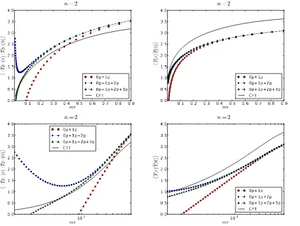
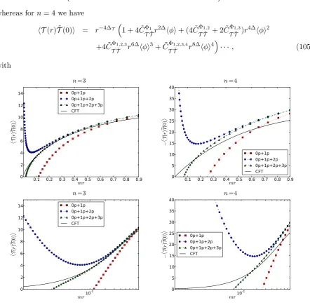
Figure 3: Zeroth order perturbed CFT versus form factor computation of the two-point function
h:Tφ: (r) : ˜Tφ: (0)i and −hT(r) ˜T(0)i. Squares, circles and triangles represent contributions up to one-, two- and three-particles to the form factor expansion. For each correlator we present results both in linear and logarithmic scale. As expected, we see that the form factor result (triangles) and the CFT computation (solid line) are in relatively good agreement for small values of mr but quickly drift apart for larger values of mr. The range of agreement is seen more clearly by using a logarithmic scale, where we can directly compare the slopes of the form factor and CFT curves.
Plugging these values in (89) as well as the expectation value (51) we obtain
hT(r) ˜T(0)i=r1110
1−(4.6566...)(mr)−45
+· · · , (94)
and
h:Tφ: (r) : ˜Tφ: (0)i=r32
1−(6.2515...)(mr)−25 + (8.5055...)(mr)− 4 5
+· · · , (95)