Hypersonic simulations using open-source CFD and DSMC solvers

Hypersonic Simulations using Open-Source CFD and DSMC

Solvers

V. Casseau

, T. J. Scanlon

, B. John

, D. R. Emerson

and R. E. Brown

1_{James Weir Fluids Laboratory, Department of Mechanical and Aerospace Engineering, University of Strathclyde,}

Glasgow, G1 1XJ, UK

2_{Centre for Future Air-Space Transportation Technology, Department of Mechanical and Aerospace Engineering,}

University of Strathclyde, Glasgow, G1 1XJ, UK

3_{Scientific Computing Department, STFC Daresbury Laboratory, Warrington, WA4 4AD, UK}

a)_{Corresponding author: [email protected]}

Abstract.

Hypersonic hybrid hydrodynamic-molecular gas flow solvers are required to satisfy the two essential requirements of any high-speed reacting code, these being physical accuracy and computational efficiency. The James Weir Fluids Laboratory at the University of Strathclyde is currently developing an open-source hybrid code which will eventually reconcile the direct simula-tion Monte-Carlo method, making use of the OpenFOAM applicasimula-tion calleddsmcFoam, and the newly coded open-source two-temperature computational fluid dynamics solver namedhy2Foam. In conjunction with employing the CVDV chemistry-vibration model inhy2Foam, novel use is made of the QK rates in a CFD solver. In this paper, further testing is performed, in particular with the CFD solver, to ensure its efficacy before considering more advanced test cases. Thehy2FoamanddsmcFoamcodes have shown to compare reasonably well, thus providing a useful basis for other codes to compare against.

INTRODUCTION

Hypersonic hybrid hydrodynamic-molecular gas flow solvers need to satisfy the two essential requirements of any high-speed reacting code, these being physical accuracy and computational efficiency. Available hybrid solvers were reviewed by Schwartzentruber and Boyd [1] and are essentially in-house codes, whilst the James Weir Fluids Labora-tory at the University of Strathclyde is currently developing an open-source hybrid code [2].

The newly coded open-source two-temperature computational fluid dynamics (CFD) solverhy2Foamhas been developed to tackle the highly complex flow physics of the hypersonic planetary atmospheric entry [3]. Implemented within the OpenFOAM framework [4], the code has the capability to model physical phenomena relative to the high-speed, chemically-reacting environment surrounding a spacecraft. The non-equilibrium conditions are treated by making the distinction between the trans-rotational and multiple vibrational-electronic energy pools. This allows the modelling of energy exchanges between the pools and the introduction a chemistry-vibration source term into the Navier-Stokes-Fourier (NSF) equations.hy2Foamhas been extensively validated for a 5-species air using fundamental zero-dimensional benchmark cases.

The purpose of this work is to compare the results given by the hy2FoamanddsmcFoamsolvers. The flow-field around a Mach 20 circular cylinder in the bottom range of the continuum-transition regime is investigated with emphasis being made on the importance of considering chemical reactions to correctly estimate the aerothermal loads.

METHODOLOGY

Conventional computational fluid dynamics

coor-dinate system for a mixture composed ofNsspecies, includingNmmolecules [5]

∂U

∂t +

∂ F_i,inv−F_i,vis

∂xi =

˙

W (1)

The vector of conserved quantities,U, is defined as

U= ρ, ρs, ρu, ρv, ρw, Eve,m, ET s∈Ns,m∈Nm (2) whereu,v, andware the components of the velocity vector.ρis the mass density of the fluid andρsis the partial density of speciess. The flux vectors are split into inviscid and viscous contributions and are written as follows

F_i,inv=

                                

ρui

ρsui

ρuiu+δi1p ρuiv+δi2p ρuiw+δi3p

Eve,mui (E+p)ui

                                

(3) F_i,vis=

                                 0

−J_s,i

τi1 τi2 τi3

−qve,m,i−eve,mJm,i

τi juj−qtr,i−qve,i−

X

r,e

hrJr,i

                                 (4)

where the indexirefers to one of the three dimensions of space andδis the Kronecker delta. Eis the total energy per unit volume whileEve,mandeve,mrepresent respectively the vibrational energy per unit volume and the vibrational energy per unit mass for speciesm.hsis the enthalpy per unit mass of speciess, while the pressure,p, is recovered from the partial pressures using Dalton’s law.J_s,iare the components of the species mass diffusion vector andτi j represents the components of the viscous stress tensor.

The source term vector,W, is written as˙

˙

W=0, ω˙s, 0, 0, 0, ω˙v,m,0

T

s∈Ns, m∈Nm (5)

where ˙ωsis the net mass production of speciessand ˙ωv,m, form∈Nm, is given by ˙

ωv,m=Qm,V−T +Qm,V−V+Qm,C−V (6)

In order of appearance in Equation 6, the source terms represent vibrational-translational (V-T) energy exchange, vibrational-vibrational (V-V) energy transfer and the vibrational-electronic energy added or removed by reactions to the speciesm. The default configuration assumes that the electronic mode is disabled. V-T energy exchange is modelled by the Landau-Teller equation [6]. The relaxation times are evaluated using either the Millikan and White [7] semi-empirical correlation with the correction of Park [8], and denoted as MWP in the following, or by the SSH theory named after Schwartz, Slawsky, and Herzfeld [9]. The coefficients of this latter model are taken from the work of Thivet [10] and a blended model is created with the MWP formulation for molecule-atom collisions. The formulation that has been implemented to account for V-V energy transfer is the one of Knabet al. [11, 12]. Finally, the chemistry source term is handled either by the Park TTv model [8] or by the coupled vibration-dissociation-vibration (CVDV) model of Marrone and Treanor [13, 14].

In hy2Foam, species thermal properties follow the Blottner [15] and Eucken [5, 16] formulas while mixture properties are recovered using the Armaly and Sutton mixing rule, as prescribed in the review from Palmer and Wright [17]. Other mixing rules such as those of Wilke [18] or Gupta [19] are also implemented but will not be considered in this work. The diffusion fluxes are governed by Fick’s law with a correction term to ensure mass conservation [20]. The binary diffusion coefficient model is the one of Hirschfelder [21].

hy2Foamuses the central-upwind interpolation schemes of Kurganov and Tadmor [22]. The non-equilibrium boundary conditions employed at the wall are the first-order Smoluchowski temperature jump [23] and the Maxwell velocity slip [24].

The direct simulation Monte Carlo method

this work is the OpenFOAM solverdsmcFoam[26]. It inherently has three temperatures: translational, rotational and vibrational. The vibrational mode has been included in the latest release as a serial application of the quantum Larsen-Borgnakke procedure. Thus, the vibrational energy can only take discrete quantum values and V-T energy exchanges rely mostly on microscopic gas information. Following on from this, the implementation of the quantum kinetic (QK) method to describe chemical reactions in a 5-species air model has been made possible.

Departure from the continuum regime

The local gradient-length Knudsen number initially proposed by Boyd [27] has extensively been used as a breakdown parameter in the literature (e.g.in [28, 29, 30, 31]). This is computed to identify the regions where the continuum assumption does not hold. For a local macroscopic flow quantityφ, it is defined as

KnGLL−φ= λ

φ|∇φ| (7)

whereλis the local mean free path of the gas molecules and in whichφcan either be the gas density, the temperature, or the magnitude of the velocity vector|U|(or max(|U|,a) in the denominator wherea is the speed of sound for low-speed regions [32]). The degree of local continuum breakdown is then evaluated as the maximum for all the aforementioned flow quantities

KnGLL=max

KnGLL−ρ,KnGLL−Ttr,KnGLL−Tve,KnGLL−|U|

(8)

This parameter will be informative in the subsequent simulations.

RESULTS

The hypersonic flow over a two-dimensional circular cylinder of radius R=1 m is being considered for analysis. The free-stream fluid is pure nitrogen. The geometry models the upper half of the domain thus taking advantage of the symmetry of the problem. The streamwise extent of the computational domain spans from -1.8 m to 5 m.

The initial conditions are listed in Table 1. The case is run at a free-stream velocity of 6,047 m s−1and pressure of 0.89 Pa. The free-stream temperatureT∞=220 K is high enough to result in a vibrationally-excited flow-field. The

cylinder wall is held at a uniform temperature of 1,000 K. The overall Knudsen number, equal to 0.0022, lies in the bottom range of the continuum-transition regime but locally the gas may lie into the transition regime.

TABLE 1.Initial conditions for the Mach 20 cylinder

Quantity Value Unit

Free-stream velocity,U∞ 6,047 m s−1

Free-stream pressure,p∞ 0.89 Pa

Free-stream density,ρ∞ 1.363×10−5 kg m−3

Free-stream temperature,T∞ 220 K

Free-stream mean-free-path,λ∞ 4.45×10−3 m

Overall Knudsen number,Knov 0.0022

-Wall temperature,Tw 1,000 K

CFD set-up

The mesh used in this investigation consisted of 40,000 cells and the first spacing at the cylinder wall was taken as 2 microns. The simulations make the use of the Maxwell velocity slip and Smoluchowski temperature jump boundary conditions with accommodation coefficients equal to 1.

TABLE 2.CFD simulations performed

Run number V-T transfer Electronic mode Rates

1 MWP no

-2 SSH no

-3 MWP yes

-4 MWP no QK

5 SSH no QK

The two chemical reactions being considered in Run number 4 and 5 are the irreversible molecule-molecule and molecule-atom dissociation of nitrogen

N₂ + N₂ −−−→ 2 N + N₂

N₂ + N −−−→ 2 N + N

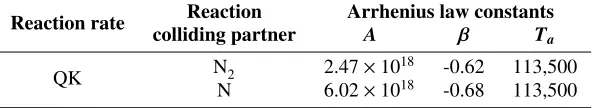
The Arrhenius rate constants are shown in Table 3 in which the units ofAandTaare given in m3mol−1s−1and Kelvin, respectively. They are derived from the QK theory [26]. Finally, the CVDV model is retained for each reacting computation.

TABLE 3.Parameters for the evaluation of the forward rate constant

Reaction rate Reaction Arrhenius law constants

colliding partner A β Ta

QK N2 2.47×10

18 _{-0.62 113,500}

N 6.02×1018 _{-0.68 113,500}

DSMC set-up

The variable hard sphere model is adopted with a temperature exponent of viscosity of 0.74, and a reference tem-perature ofTre f =273 K. The particles impinging the cylinder wall are reflected diffusely with an accommodation coefficient equal to 1. Good DSMC practice have been satisfied for the mesh and the time-step. The cell size is equal to a third of the mean-free-path and a spline was used to minimize the region being modelled upstream the bow shock. The DSMC mesh then consisted of 5.5 million cells. Each cell was filled with approximately 15 equivalent DSMC particles which resulted in simulations using over 80 million particles. The DSMC time-step was set to 1/5 of the mean-free-time.

Analysis

Non-reacting case scenarios

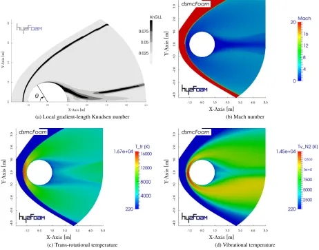
The regions where the flow departs significantly from local thermodynamic equilibrium are highlighted in Fig. 1(a) using the local gradient-length Knudsen number and later shown in Fig. 2. This indicates that the CFD solver will be unlikely to provide satisfactory results within the bow shock and in the near-wake of the cylinder, as shown by

KnGLL values above 0.05. In particular, the low density region forθ'130 deg is driving theKnGLLbeyond 10. For the reacting case scenario, a very similar picture ofKnGLLis observed.

(a) Local gradient-length Knudsen number (b) Mach number

(c) Trans-rotational temperature (d) Vibrational temperature

FIGURE 1.CFD-DSMC flow-field comparisons for Run number 2 (non-reacting).

Figure 2(a) - 2(c) compares the stagnation line profiles of temperature, number density, and Mach number provided by hy2Foamand dsmcFoam for the run number 2. They are all in very good agreement outside of the

KnGLL>0.1 band.

Effect of chemical reactions

Figure 2(d) - 2(f) now include the effect of the two dissociation reactions considered. The shock stand-offdistance is reduced from 0.29 m to 0.25 m. Due to the significantly thin bow shock using CFD, the steep increase inTtris delayed and the small production of atomic nitrogen within the shock is thus not captured, as seen in Fig. 2(d). The vibrational temperature profile is less accurately estimated as compared with the non-reacting case.

Temperature [K x 10

3]

Stagnation line position [m] non-reacting N2

dsmcFoam, Ttr T_v hy2Foam, Ttr Tv

0 5 10 15

-1.5 -1.4 -1.3 -1.2 -1.1 -1

KnGLL > 0.01 KnGLL > 0.1

(a) Run 2: Temperature

Normalised number density,

n

/

n∞

Stagnation line position [m] non-reacting N2

dsmcFoam hy2Foam

100 101 102

-1.5 -1.4 -1.3 -1.2 -1.1 -1

KnGLL > 0.1

KnGLL > 0.01

(b) Run 2: Normalised number density

Mach

Stagnation line position [m]

non-reacting N2

dsmcFoam hy2Foam

0 5 10 15 20

-1.5 -1.4 -1.3 -1.2 -1.1 -1

KnGLL > 0.1

KnGLL > 0.01

(c) Run 2: Mach number

Mach

Stagnation line position [m]

reacting N2

dsmcFoam hy2Foam

0 5 10 15 20

-1.5 -1.4 -1.3 -1.2 -1.1 -1

KnGLL > 0.1

KnGLL > 0.01

(d) Run 5: Mach number

Temperature [K x 10

3]

Stagnation line position [m] reacting N2

dsmcFoam, Ttr Tv,N2 hy2Foam, Ttr Tv,N2

0 5 10 15

-1.5 -1.4 -1.3 -1.2 -1.1 -1

KnGLL > 0.01 KnGLL > 0.1

(e) Run 5: Temperature

Number density [m

-3]

Stagnation line position [m]

reacting N2

dsmcFoam, N2 N

hy2Foam, N2 N

1018 1019 1020 1021 1022

-1.5 -1.4 -1.3 -1.2 -1.1 -1

KnGLL > 0.1

KnGLL > 0.01

(f) Run 5: Number density

Pressure coefficient

Theta [deg]

free-stream: N2

dsmcFoam, NR QK

hy2Foam, NR QK

0 0.5 1 1.5 2

0 30 60 90 120 150 180

(a) Pressure coefficient

Friction coefficient

Theta [deg]

free-stream: N2

dsmcFoam, NR QK

hy2Foam, NR QK

0 0.01 0.02 0.03 0.04 0.05 0.06

0 30 60 90 120 150 180

(b) Skin-friction coefficient

Surface Heat Flux [W/cm

2]

Theta [deg]

free-stream: N₂

dsmcFoam, NR QK

hy2Foam, NR QK

0 5 10 15

0 30 60 90 120 150 180

(c) Surface heat transfer

FIGURE 3.Surface quantities around the cylinder (run numbers 2 and 5).

TABLE 4.Global aerothermodynamic coefficients

CFD run number CD(pressure contribution) CH[kW]

CFD DSMC CFD DSMC

1 1.3(96.8%)

1.286(97.5%) 115 115

2 1.296(96.8%) 109

3 1.308(96.8%) × 114 ×

4 1.3(96.8%)

1.284(97.8%) 66.5 63.3

5 1.296(96.8%) 68.2

CONCLUSIONS

Thehy2FoamanddsmcFoamresults have shown to be in reasonable concordance, thus verifying the implementation of hy2Foamfor two-dimensional geometries in a reacting and neutral environment. The use of the CVDV model for chemistry-vibration coupling together with reaction rates derived from Quantum-Kinetics -through the use of

ACKNOWLEDGMENTS

The CFD results were obtained using the EPSRC funded ARCHIE-WeSt High Performance Computer (www.archie-west.ac.uk/). EPSRC grant no. EP/K000586/1. This work has also been awarded an ARCHER Resource Alloca-tion Panel (RAP) grant. D. R. Emerson and B. John thank EPSRC for support under grants EP/N016602/1 and EP/K038427/1. V. Casseau would like to acknowledge Daniel E. R. Espinoza and Jimmy-John Hoste for their help in testing thehy2Foamsolver.

REFERENCES

[1] T. Schwartzentruber and I. D. Boyd, Progress in Aerospace Sciences72, 66–79 (2014).

[2] D. E. R. Espinoza, V. Casseau, T. J. Scanlon, and R. E. Brown, “An Open Source Hybrid CFD-DSMC Solver for High-Speed Flows,” inProceedings of the 30th Rarefied Gas Dynamics Conference, Paper 2964 (Victoria BC, Canada, July 10-15, 2016).

[3] V. Casseau, T. J. Scanlon, and R. E. Brown, “Development of a Two-Temperature Open-Source CFD Model for Hypersonic Reacting Flows,” AIAA Paper 2015-3637 (2015).

[4] OpenFOAM official website, http://www.openfoam.com/( accessed: 12 January 2016).

[5] G. V. Candler and I. Nompelis, “Computational Fluid Dynamics for Atmospheric Entry,” RTO-EN-AVT-162 (2009).

[6] L. Landau and E. Teller, Physikalische Zeitschrift der Sowjetunion10(1936).

[7] R. C. Millikan and D. R. White, The Journal of Chemical Physics39, 3209–3213 (1963).

[8] C. Park,Nonequilibrium Hypersonic Aerothermodynamics(Wiley International, New York, 1990).

[9] R. N. Schwartz, Z. I. Slawsky, and K. F. Herzfeld, The Journal of Chemical Physics20, 1591–1599 (1952). [10] F. Thivet, M. Y. Perrin, and S. Candel, Physics of Fluids3, 2799–2812 (1991).

[11] O. Knab, H.-H. Fr¨uhauf, and S. Jonas, “Multiple Temperature Descriptions of Reaction Rate Constants with Regard to Consistent Chemical-Vibrational Coupling,” AIAA Paper 92-2947 (1992).

[12] O. Knab, H.-H. Fr¨uhauf, and E. W. Messerschmid, Journal of Thermophysics and Heat Transfer9, 219–226 (1995).

[13] C. E. Treanor and P. V. Marrone, Physics of Fluids9, 1022–1026 (1962). [14] P. V. Marrone and C. E. Treanor, Physics of Fluids6, 1215–1221 (1963).

[15] F. G. Blottner, M. Johnson, and M. Ellis, “Chemically reacting viscous flow program for multicomponent gas mixtures,” Report No. SC-RR-70-754 (Albuquerque, New Mexico, 1971).

[16] W. G. Vincenti and C. H. Kruger, Introduction to Physical Gas Dynamics(Krieger Publishing Company, Florida, 1965).

[17] G. E. Palmer and M. J. Wright, Journal of Thermophysics and Heat Transfer17, 232–239 (2003). [18] C. R. Wilke, Journal of Chemical Physics18, 517–519 (1950).

[19] R. Gupta, J. M. Yos, R. A. Thompson, and K.-P. Lee, “A Review of Reaction Rates and Thermodynamic and Transport Properties for an 11-Species Air Model for Chemical and Thermal Nonequilbrium Calculations to 30000 K,” Tech. Rep.

[20] K. Sutton and P. A. Gnoffo, “Multi-component Diffusion with Application to Computational Aerothermody-namics,” AIAA Paper 98-2575 (1998).

[21] J. O. Hirschfelder, C. Curtiss, and R. B. Bird,Molecular Theory of Gases and Liquids(John Wiley & Sons, Inc., 1954).

[22] A. Kurganov, S. Noelle, and G. Petrova, SIAM J. Sci. Comput.23, 707–740 (2001). [23] M. von Smoluchowski, Annalen der Physik und Chemie64, 101–130 (1898). [24] J. C. Maxwell, Phil. Trans. R. Soc. Lond.170, 231–256 (1879).

[25] G. A. Bird,Molecular gas dynamics and the direct simulation of gas flows(Clarendon, Oxford, 1994). [26] T. J. Scanlonet al., AIAA Journal53, 1670–1680 (2015).

[27] I. D. Boyd, G. Chen, and G. V. Candler, Physics of Fluids7, 210–219 (1995).

[28] T. E. Schwartzentruber, L. C. Scalabrin, and I. D. Boyd, J. Comput. Phys.225, 1159–1174 (2007).

[29] G. Abbate, B. J. Thijsse, and C. R. Kleijn, “Computational Science – ICCS 2007: 7th International Con-ference, Beijing, China, May 27 - 30, 2007, Proceedings, Part I,” (Springer Berlin Heidelberg, Berlin, Hei-delberg, 2007) Chap. Coupled Navier-Stokes/DSMC Method for Transient and Steady-State Gas Flows,, pp. 842–849.

[30] M. Darbandi and E. Roohi, Sensors and Actuators A189, 409–419 (2013).

[31] R. Roveda, D. B. Goldstein, and P. L. Varghese, J. Spacecraft Rockets35, 258–265 (1998).