Entropic approximation for mathematical programs with robust equilibrium constraints

City, University of London Institutional Repository

Citation:

Liu, Y. and Xu, H. (2014). Entropic approximation for mathematical programs

with robust equilibrium constraints. SIAM Journal on Optimization, 24(3), pp. 933-958. doi:

10.1137/130931011

This is the accepted version of the paper.

This version of the publication may differ from the final published

version.

Permanent repository link:

http://openaccess.city.ac.uk/3267/

Link to published version:

http://dx.doi.org/10.1137/130931011

Copyright and reuse: City Research Online aims to make research

outputs of City, University of London available to a wider audience.

Copyright and Moral Rights remain with the author(s) and/or copyright

holders. URLs from City Research Online may be freely distributed and

linked to.

EQUILIBRIUM CONSTRAINTS

YONGCHAO LIU∗ _{AND HUIFU XU}†

Abstract. In this paper, we consider a class of mathematical programs with robust equilibrium constraints represented by a system of semi-infinite complementarity constraints (SICC). We propose a numerical scheme for tackling SICC. Specifically, by relaxing the complementarity constraints and then randomizing the index set of SICC, we employ the well-known entropic risk measure to approximate the semi-infinite constraints with a finite number of stochastic inequality constraints. Under some moderate conditions, we quantify the approximation in terms of the feasible set and the optimal value. The approximation scheme is then applied to a class of two stage stochastic mathematical programs with complementarity constraints in combination with the polynomial decision rules. Finally, we extend the discussion to a mathematical program with distributionally robust equilibrium constraints which is essentially a one stage stochastic program with semi-infinite stochastic constraints indexed by some probability measures from an ambiguity set defined through the KL-divergence.

Key words.Entropic risk measure, robust equilibrium constraints, polynomial decision rule, stability analysis, KL-divergence.

AMS subject classifications.90C15, 90C30, 90C33.

1. Introduction. Consider the following mathematical program with semi-infinite complementarity con-straints

(MPSICC) min

x∈X f(x)

s.t. 0_≤x_⊥g(x, t)_≥0, _∀t_∈T, (1.1)

where X is a nonempty compact set of IRn, f : IRn → IR and g : IRn×T → IRn are continuous functions, T is a compact index set and a _⊥ b denotes orthogonality of vectors a and b. In practical applications, the complementarity constraints are often used to describe an equilibrium arising from economic competition or traffic flow, whereas the index parameter t may represent various uncertainties such as market demand, economic or environmental conditions. Consequently MPSICC may be called a mathematical program with robustcomplementarity constraints where the robustness is in the sense that the constraints must hold for every realization of the uncertain parameter. In the case when T is a finite set, (1.1) is known as a mathematical program with complementarity constraints (MPCC) which has been extensively investigated over the past two decades, see monographs [28, 30] for a comprehensive treatment of the topic.

Our interest in this paper is on the case when T is an infinite set. To ease the exposition, we assume that T is a compact set of a finite dimensional space although most of our technical results hold whenT is a subset of a Banach space. The MPSICC may be viewed as an extension of the mathematical programs with robust equality and/or inequality constraints which has been investigated extensively over the past two decades [1, 5, 6, 7, 8, 12, 13, 14, 16, 20, 45]. For instance, in multiload truss optimization, mechanical response of a truss is often represented by a robust linear system of equations parameterized by nodal displacement vector, which is a special case of robust complementarity constraints.

Our focus in this paper is on the numerical methods for solving MPSICC. Note that the optimization problems with robust constraints in [12, 2] are convex while problem (1.1) is typically nonconvex because of combinatorial structure of the complementarity constraints. Moreover, the feasible set of the problem does not have an interior which means that a direct application of a randomization approach is often numerically unstable. To address the issue, we employ the well known NLP-regularization scheme (see [36]) to relax the complementarity constraints by replacing them with a parameterized semi-infinite system of inequalities:

(RMPSICC) min

x∈X+

f(x)

s.t. −_xg(x, t)≤0 ◦g(x, t)_≤τ e

∀t∈T, (1.2)

∗_{Department of Mathematics, Dalian Maritime University, Dalian 116026, China ([email protected]). The work of this}

author is supported by NSFC 11201044 and FRFCU 3132014037.

†_{School of Engineering and Mathematical Sciences, City University London, EC1V 0HB, London, UK ([email protected]).}

The work of this author is supported by EPSRC grant EP/J014427/1.

whereX+:=X∩IRn+, IR

n

+ denotes the set of n-dimensional vectors whose components are nonnegative,τ≥0

is a fixed positive parameter,e_∈IRn is a vector with components 1 and “_◦” denotes the Hadamard product. The regularized problem RMPSICC has at least two advantages from numerical point of view: (a) it involves ordinary inequality constraints, and (b) its feasible solution set is more likely to have an interior as opposed to MPSICC. Under some moderate conditions, RMPSICC approximates MPSICC asτ is driven to zero. We will come back to the details of this in Section 3. For a fixed parameterτ, we propose a randomization approach based on the entropic risk measure to solve RMPSICC. Specifically, by treatingtas a random parameter1_{, we}

use the entropic risk measure ofg(x, t) andx_◦g(x, t) to approximate the semi-infinite constraints of RMPSICC.

Much of the rest of the work is on the theoretical analysis of the entropic approximation of RMPSICC as the entropic risk measure parameter varies in terms of the optimal value and the optimal solutions (Section 3). Moreover, we propose a sample average approximation (SAA for short) for the entropic risk measure and investigate the convergence of the optimal value and the optimal solutions as the sample size increases (Section 3). As an application, we apply the proposed numerical schemes to a two stage stochastic mathematical program with complementarity constraints in a combination with the well known polynomial decision rule method [4] (Section 4) and to a stochastic mathematical program with distributionally robust equilibrium constraints where the distributional set is constructed through a nominal sample average approximated distribution within a range specified through the Kullback-Leibler divergence (Section 5). As far as we are concerned, the main contributions of the paper can be summarized as follows:

• Entropic approximation for MPSICC.

MPSICC(1.1)_−−−→Reg RMPSICC(1.2)_{−−−−−−−−−−→}Entropic Appr

SAA SAA-EA-RMPSICC(3.4).

We propose a new optimization model with robust complementarity constraints (1.1) which extends the existing optimization models with robust inequality and/or equality constraints. We develop a numerical scheme for solving the problem (1.1) which utilizes the entropic risk measure and sample average approximation, and carry out qualitative and quantitative stability analysis of the approximation scheme in terms of the optimal value and the optimal solutions. Differing from the mainstream approaches in distributionally robust optimization, the approximation scheme does not require dualization for transforming the semi-infinite constraint into a semi-definite constraint and hence can be applied to a nonconvex function g(x, t). It also differs from Calafiore and Campi’s randomization method [12, 13] in that the resulting optimization problem does not increase the number of constraints as the sample size increases, and the use of the entropic risk measure may lead to stability of the optimal values. • Entropic approximation for two stage SMPECs.

SMPEC(4.1)_−−−→Reg

PDL PDL-RSMPEC(4.3)

Entropic Appr

−−−−−−−−−−→_SAA SAA-EA-PDL-RSMPEC(4.6).

By applying the numerical scheme in a combination with the polynomial decision rule (PDL) [4] and the sample average approximation method to a two stage stochastic mathematical program with com-plementarity constraints (SMPEC), we provide an alternative method to tackle two stage SMPECs which are often notoriously difficult to solve. A significant advantage of the new framework is that it does not scale in the number of the sample size.

• Entropic approximation for one stage mathematical programs with distributionally robust equilibrium constraints (MPDRE).

MPDRE(5.1)_−−−→Reg RMPDRE(5.3)_{−−−−−−−−−−→}Entropic Appr

SAA SAA-EA-EMPDRE(5.7).

The MPDRE model provides a mathematical tool for the study of robust equilibria. It has potential applications in market design where equilibria withstand uncertain economic circumstances. The new model and the numerical scheme extend the recent research on optimization problems with distribu-tionally robust inequality constraints by Hu and Hong [21].

Throughout the paper, we will use the following notation. We denote by_k·kthe Euclidean norm of a vector, d(x, D) the distance from a point xto a set D and Diam(D) the diameter of the set D, that is, d(x, D) := infx′∈Dkx−x′kand Diam(D) := supx′,x′′∈Dkx′−x′′k. For two compact setsD1andD2, we writeD(D1, D2) the

1

deviation ofD1fromD2, that is,D(D1, D2) := supx∈D1d(x, D2) andH(D1, D2) := max (D(D1, D2),D(D2, D1))

for the Hausdorff distance betweenD1 andD2. Finally, we use standard notation clD for the closure of set D

and limk→∞Dk for the outer limit of a sequence of sets{Dk}.

2. Entropic risk measure approximation. Let M denote the linear space of bounded measurable functions defined on some measurable space (Ω,F). Consider a setA ⊂Msuch that

Z ∈ A, U ∈M, U ≥Z=⇒U ∈ A.

Define the functionalρ:M→IR byρ(Z) := inf{m∈IR :Z+m∈ A}.It is easy to verify thatρ(Z1)≤ρ(Z2),

forZ1≥Z2andρ(Z+m) =ρ(Z)−m.In the literature of finance risks,ρ(·) is known as a monetary risk measure

whenZ represents a financial position, e.g., capital, see [18]. Letγbe a positive number andu(z) = 1₋e−γz

be an exponential utility function. If we define A := {Z ∈ L∞ : |EP[u(Z)]| ≥ u(0)}, then the resulting risk

measure is

eγ(Z) :=ρ(Z) = 1

γlnEP[e

−γZ_{] (2.1)}

forZ∈L∞_{. The risk measure has a robust representation}

eγ(Z) = sup Q∈M1

{EQ[Z]−

1

γH(Q|P)},

where_M1 denotes the set of all probability measures onM, and

H(Q_|P) :=

(

EQ

h

lndQ_dPi, forQP

+_∞, otherwise (2.2)

denotes the relative entropy ofQwith respect to P, QP meansQis absolutely continuous with respect to P. Consequentlyeγ(Z) is called entropic risk measure, see [17] for a thorough treatment of the concept. It is

well known (see e.g. [18, formulation (4)]) thateγ(Z) is monotonically increasing inγand

lim

γ→∞eγ(Z) = ess sup(−Z) (2.3)

in the case that ess infZ > _−∞. Our focus in this paper is mainly on the limit rather than the financial background of the risk measure.

Leth: IRn_×IRk _→IR be a continuous function andX be a subset of IRn. Let ξ: Ω_→IRk be a random variable defined on the probability space (Ω,F, P) with support set Ξ. Our interest is the uniformity of limit (2.3) whenz=h(x, ξ) w.r.t. x. We address this in the following proposition.

Proposition 2.1. (Entropic approximation of random functions)Let H(x), Fx(t) andΩx denote respectively the essential supremum, the cumulative distribution function and the support set of ₋h(x, ξ). Let Diam(Ωx)denote the diameter of the support setΩxwhich is the distance between H(x)and essential infimum of ₋h(x, ξ). Assume: (a)X _⊂IRn be a compact set, (b) for each fixedx_∈X,

inf

ξ∈Ξh(x, ξ)>−∞. (2.4)

Then for each fixedx_∈X,

lim

γ→∞eγ(h(x, ξ)) =H(x). (2.5)

Assume in addition that (c)

inf

x∈Xξinf∈Ξh(x, ξ)>−∞, (2.6)

and (d) for any fixed small positive numberǫ, there existsδ(ǫ)_∈(0,1) such that

whereXǫ:={x∈X: Diam(Ωx)>2ǫ}. Then

|eγ(h(x, ξ))−H(x)|<2ǫ+

1

γ|lnδ(ǫ)|. (2.8)

Proof. The convergence (2.5) is well known, see the comments following [18, Formulation (4)]. Here, we provide a proof for completeness. We proceed the proof in two steps according to the distribution ofξ.

Step 1. ξ follows a discrete distribution, that is, Prob

ξ=ξj = pj, j = 1,2,· · · . This includes both

infinite and finite distribution (in which casepj = 0 whenj ≥k for somek). Letxbe fixed andǫ be a fixed

small positive number. LetJǫ(x) := min{j:−h(x, ξj)≥H(x)−ǫ}.Then

eγ(h(x, ξ))≥

1 γln



 X

j∈Jǫ(x)

eγ(−h(x,ξj))pj



=H(x) +

1 γln



 X

j∈Jǫ(x)

eγ(−h(x,ξj)−H(x))pj



.

Since₋h(x, ξj₎

−H(x)_{≥ −}ǫforj_{∈ J}ǫ(x), then

0> 1 γln



 X

j∈Jǫ(x)

eγ(−h(x,ξj)−H(x))pj



>−ǫ+

1 γln



 X

j∈Jǫ(x)

pj



. (2.9)

Note that for fixedx,P

j∈Jǫ(x)pj>0. Therefore, by drivingγ to∞, we obtain

0> lim

γ→∞ 1 γln   X

j∈Jǫ(x)

eγ(−h(x,ξj_)−H(x)) pj



≥ −ǫ,

which implies (2.5) becauseǫcan be arbitrarily small.

To show (2.8), we note that under condition (2.7),

1 γ ln   X

j∈Jǫ(x)

pj  

≤ 1_γ|lnδ(ǫ)|, ∀x∈Xǫ,

whereXǫ6=∅. Through (2.9), the inequality above implies (2.8). Whenx∈X\Xǫ, Diam(Ωx)≤2ǫ. Since

E[−h(x, ξ)]≤eγ(h(x, ξ))≤H(x), ∀γ >0,

then

|eγ(h(x, ξ))−H(x)| ≤2ǫ <2ǫ+

1

γ|lnδ(ǫ)|. (2.10)

Summarising the two cases, we have shown that (2.8) holds for allx∈X under condition (2.7).

Step 2. ξfollows a continuous distribution2_{. Observe first that (2.10) holds regardless of the distribution}

ofξ. Therefore, we only need to consider the case whenx∈Xǫ. Recall thatFx(t) is the cumulative distribution

function of₋h(x, ξ). It is easy to verify that

E[e−γh(x,ξ)] =eγH(x)

"

1₋γ

Z H(x)

−∞

eγ(t−H(x))Fx(t)dt

# . Therefore 1 γln

E[e−γh(x,ξ)]=H(x) +1

γln 1−γ

Z H(x)

−∞

Fx(t)eγ(t−H(x))dt

!

.

2

Letǫbe a small positive number. Then

γ

Z H(x)

−∞

Fx(t)eγ(t−H(x))dt=γ

Z H(x)−ǫ

−∞

Fx(t)eγ(t−H(x))dt+γ

Z H(x)

H(x)−ǫ

Fx(t)eγ(t−H(x))dt

≤Fx(H(x)−ǫ)e−γǫ+ 1−e−γǫ,

where the inequality follows from the monotonicity of the cumulative distribution function and the exponential function. Therefore

1 γln

E[e−γh(x,ξ)]−H(x)

<

1

γln(1−(1−e −γǫ₎

−Fx(H(x)−ǫ)e−γǫ)

=ǫ+1

γ|ln(1−Fx(H(x)−ǫ))|.

For fixedx, since 1₋Fx(H(x)−ǫ)>0, we arrive at (2.5) by drivingγto infinity and thenǫto zero. The error

bound (2.8) follows from the inequality above under condition (2.7).

Note that condition (2.7) is similar to the so called consistent tail behaviour condition for CVaR approxi-mation of the essential supremum of a random function in [2]. Indeed, the latter implies the former. We explain how the condition may be satisfied through a simple example varied from [2, Example 1].

Example 2.1. Consider h(x, ξ) = ₋xξ, where x_∈ [0,1]_⊂ IR and ξ follows a uniform distribution over interval[₋1,1]. Letǫ <1be a small positive number. ThenH(x) =x,Ωx= [−x, x]andXǫ={x∈[0,1] : 2ǫ <

2x}= (ǫ,1]. It is easy to derive that

1₋Fx(H(x)−ǫ) = ǫ 2x ≥

ǫ

2, ∀x∈Xǫ.

This shows that condition (2.7) holds with δ(ǫ) = ǫ₂. Let us now consider the case whenx∈[0,1]\Xǫ= [0, ǫ]. Then Diam(Ωx) = 2x≤2ǫand hence|eγ(h(x, ξ))−H(x)| ≤2ǫ.

Proposition 2.1 says that under some moderate conditions, the entropic risk measure of h(x, ξ) converges to the essential supremum of ₋h(x, ξ) uniformly w.r.t. xas γ _{→ ∞}. Under the similar condition, Anderson et al. [2] presented some conditions which ensure the CVaR of a random function converges uniformly to its essential supremum. The main differences are two fold: (a) CVaR utilizes the tail distribution whereas entropic approximation uses the whole distribution with more weights on the tail whenγis large. (b) CVaR is nonsmooth as it only uses the tail distribution while the entropic risk measure is smooth.

3. Stability analysis. In this section, we use the entropic risk measure as the workhorse to construct an approximation of the robust semi-infinite constraints of problem (1.2). We examine the accuracy and efficiency of the approximation from a stability point of view.

3.1. Stability w.r.t. parameters τ and γ. Let us start by writing problem (1.2) equivalently as

(RMPSICC) min

x∈X+

f(x) s.t. sup

t∈T

x◦g(x, t)≤τ e, sup

t∈T−

gj(x, t)≤0, forj∈ {1,· · ·, n},

(3.1)

where X+ :=X ∩IRn+. The proposition below states the approximation of RMPSICC (3.1) to MPSICC (1.1)

in terms of the optimal value and the optimal solutions asτ is driven to 0.

Proposition 3.1. (Stability of RMPSICC (3.1)) Let X(τ) and X∗ _{denote the sets of the optimal} solutions to the problems (3.1) and (1.1) respectively. Letv(τ)andv∗ _{denote the corresponding optimal values.} Then limτ→0X(τ)⊂X∗ andlimτ→0v(τ) =v∗.

Proof. Let_F(τ) and_Fdenote the feasible sets of the problems (3.1) and (1.1) respectively. Since_{F ⊂ F}(τ), it follows by [43, Lemma 4.2(i)], limτ→0H(F(τ),F) = 0.Letxτ ∈X(τ) andy∗∈X∗. Assume for the simplicity

of exposition (by taking a subsequence if necessary) thatxτ→x∗. Sincex∗∈ F andy∗∈ F(τ), then

f(y∗)≤f(x∗) = lim

τ→0f(xτ)≤f(y

This showsf(x∗_{) =f(y}∗_{) hence x}∗_∈X∗_{. The convergence of the optimal value also follows.}

In what follows, we regardtas a random variable with support setT and approximate the supermum with the entropic risk measure, namely,

(EA-RMPSICC) min

x∈X+

f(x)

s.t. e

j γ(x)≤0

¯

ejγ(x)≤τ

forj_{∈ {}1,_{· · ·}, n_}, (3.2)

whereγ is a fixed positive parameter,

ej

γ(x) :=eγ(gj(x, t)), e¯γj(x) :=eγ(−xj·gj(x, t)),

and eγ(·) is defined in equation (2.1). Compared to RMPSICC (3.1), EA-RMPSICC (3.2) consists of two

ordinary stochastic constraints where the underlying functions are continuously differentiable and can be ap-proximated through sampling. Moreover, the stability results to be established in this section do not depend on the probability distribution oft, which meanstcan be any random variable whose support set isT. Our focus in this section is to look into the approximation of the optimal value and the optimal solutions of EA-RMPSICC (3.2) to those of RMPSICC (3.1) asγ increases. Observe that the two problems have identical objective func-tions. Therefore it suffices to investigate the approximation of feasible constraints/solutions and its impact on the optimal value and the optimal solutions.

Let F(τ) andFγ(τ) denote the feasible solution sets of problems (3.1) and (3.2) respectively. Obviously F(τ) _{⊆ F}γ(τ). In other words, Fγ(τ) provides an outer bound for F(τ). The following proposition gives a

quantitative description of the excess ofFγ(τ) overF(τ).

Proposition 3.2. (Error bound of the feasible solution set of EA-RMPSICC (3.2)) Let F1j x (t) andF2j

x (t) denote the cumulative distributions of gj(x, t) andxjgj(x, t)respectively for j = 1,· · ·, n. Assume there exists a positive constantC such that

d(x,_F(τ))_≤C n

X

j=1

sup

t∈T− gj(x, t)

+

+

sup

t∈T

xj·gj(x, t)−τ

+

!

(3.3)

and for any fixed positive numberǫ, there existsδ(ǫ)_∈(0,1) such that forj = 1,_{· · ·} , n,

1−Fx1j

sup

t∈Tgj(x, t)−ǫ

≥δ(ǫ), ∀x∈Xǫ1j

1₋Fx2j

sup

t∈T

xjgj(x, t)−ǫ

≥δ(ǫ), _∀x_∈Xǫ2j,

where X1j

ǫ := {x ∈ X+ : Diam(Ω1xj) > 2ǫ}, Xǫ2j := {x ∈ X+ : Diam(Ω2xj) > 2ǫ} and Ω1xj and Ω2xj are the support sets of random variablesgj(x, ξ)andxjgj(x, ξ)respectively. Then

(i) for anyǫ∗_{>0, there exists a positive numberγ}

ǫ∗ such that H(Fγ(τ),F(τ))≤ǫ∗ whenγ≥γǫ∗;

(ii) H(_Fγ(τ),F(τ))≤C∆γ, where∆γ:= 4nǫ+2_γn|lnδ(ǫ)|,andnis the dimension of variable x.

The condition (3.3) is an error bound for the system of inequalities in the constraints. This type of conditions has been well studied in the past decade, see survey papers [3, 31] for more details.

Proof. Part (i). Letǫ∗_{be a fixed small positive number. Define}

Rj(ǫ∗) := inf x∈X+

d(x,F(τ))≥ǫ∗

sup

t∈T−gj(x, t),

¯

Rj(ǫ∗) := inf x∈X+

d(x,F(τ))≥ǫ∗

sup

t∈T

xj·gj(x, t)−τ,

and R(ǫ∗_{) := max}

j∈{1,···,n}max{Rj(ǫ ∗_),R¯

j(ǫ∗)}. Let δ := R(ǫ∗)/2. Then δ > 0. By Proposition 2.1, ejγ(x) and

¯ ej

there exists a sufficiently largeγǫ∗ such that

sup

x∈X+

j∈{1,···,n}

sup

t∈T−

gj(x, t)−ejγ(x)

≤δ

and

sup

x∈X+

j∈{1,···,n}

sup

t∈T

xj·gj(x, t)−¯ejγ(x)

≤δ,

whenγ_≥γǫ∗.

Letx_∈X+ be such that d(x,F(τ))≥ǫ∗ and γ≥γǫ∗. There existsj ∈ {1,· · ·, n}such that at least one

of the following inequalities holds

¯ ej

γ(x)−τ= sup t∈T

xj·gj(x, t)−τ+ ¯ejγ(x)−sup t∈T

xj·gj(x, t)≥R(ǫ∗)−R(ǫ∗)/2 =R(ǫ∗)/2>0,

ejγ(x) = sup t∈T−

gj(x, t) +ejγ(x)−sup t∈T−

gj(x, t)≥R(ǫ∗)−R(ǫ∗)/2 =R(ǫ∗)/2>0,

which meansx_{6∈ F}γ(τ), or equivalently,d(x,F(τ))< ǫ∗ for everyx∈ Fγ(τ). This showsD(Fγ(τ),F(τ))≤ǫ∗

and hence H(F(τ),Fγ(τ))≤ǫ∗ givenF(τ)⊆ Fγ(τ).

Part (ii). Observe that_F(τ)_{⊆ F}γ(τ). Hence, it suffices to proveD(Fγ(τ),F(τ))≤C∆γ. Let ˆx∈ Fγ(τ).

Forj= 1,_{· · ·}, n,ej

γ(ˆx)≤0 and ¯ejγ(ˆx)−τ ≤0.Through (2.8), we have

sup

t∈T−

gj(ˆx, t)−ejγ(ˆx)

≤

2ǫ+1 γ

ln(1₋F_xˆ1j(sup

t∈T−

gj(ˆx, t)−ǫ))

and sup

t∈T

ˆ

xj·gj(ˆx, t)−¯ejγ(ˆx)

≤

2ǫ+ 1 γ

ln(1₋F_ˆx2j(sup

t∈T

ˆ

xj·gj(ˆx, t)−ǫ))

.

By exploiting the inequalities above and the condition (3.3), we arrive at

d(ˆx,_F(τ))_≤C n

X

j=1

sup

t∈T− gj(ˆx, t)

+

+

sup

t∈T

xj·gj(ˆx, t)−τ

+ ! ≤C   n X j=1 sup

t∈T−

gj(ˆx, t)−ejγ(ˆx)

+

+

sup

t∈T

xj·gj(ˆx, t)−e¯jγ(ˆx)

+





≤4nǫ+2n

γ ln|δ(ǫ)|.

The proof is complete.

Proposition 3.2 says that the feasible set mapping of EA-RMPSICC (3.2) converges to the feasible set of RMPSICC (3.1) asγ→ ∞. Using this property, we can establish the convergence of the optimal value and the optimal solutions.

Theorem 3.1. (Stability of EA-RMPSICC (3.2)) Let Xγ(τ) and X(τ) denote the sets of optimal solutions of the problems (3.2) and (3.1) respectively, vγ(τ) and v(τ) be the corresponding optimal values. Assume the conditions of Proposition 3.2. Then

(i) limγ→∞vγ(τ) =v(τ) and limγ→∞Xγ(τ)⊆X(τ);

Proof. Part (i). It is sufficient to show the convergence of the optimal solutions as f(·) is continuous and independent ofγ. Assume a contradiction that there existsxN

∈ XγN(τ) such that x N

→x∗ _andx∗

6∈X(τ), whereγN →+∞. By Proposition 3.2,x∗∈ F(τ). Moreover, there exists ¯x∈X(τ) such thatf(x∗)−f(¯x)>0.

On the other hand, since ¯x_{∈ F}(τ)_{⊂ F}γN(τ),f(x N₎

−f(¯x)_≤0.This contradicts an earlier inequality whenN is sufficiently large.

Part (ii). The conclusion essentially follows from Part (i) and [22, Theorem 1]. Here we include a brief proof for completeness. Letxγ andx0be the optimal solutions of the problems (3.2) and (3.1) respectively. By

part (ii) of the proposition 3.2 , there exists ¯xγ ∈ F(τ) such thatkxγ−x¯γk ≤C∆γ.Moreover

v(τ)≤f(¯xγ)≤f(xγ) +|f(¯xγ)−f(xγ)| ≤vγ(τ) +LC∆γ.

Under the symmetry of the Hausdorff distance betweenFγ(τ) andF(τ), we can showvγ(τ)≤v(τ) +LC∆γ.

The conclusion follows.

In the classical stability analysis of nonlinear programming, it is often assumed some kind of growth con-ditions for the objective function in order to derive the stability of the optimal solution, see for instance Klatte [22, Theorem 2]. In this context, the growth condition would be

f(x′)_≥ min

x∈F(τ)f(x) +αd(x

′_{, X(τ)).}

Since problems (3.1) and (3.2) have identical objective functions while the feasible set of the former is contained in that of the latter, the growth condition would force the set of optimal solutions to the problem (3.2) to stay on the set of optimal solutions to the problem (3.1). To see this more clearly, let ¯x _∈ Xγ(τ) be an optimal

solution to the problem (3.2). SinceX(τ)_{⊂ F}γ(τ), the growth condition means

0≥vγ(τ)−v(τ) =f(¯x)−v(τ)≥αd(¯x, X(τ)),

which yields ¯x_∈X(τ) and hence Xγ(τ)≡X(τ).

3.2. Sample average approximation. In some circumstances, it might be numerically too expensive to calculate the expected values in the entropic function. A well-known approximation method to deal with the mathematical expectation in stochastic programming is the sample average approximation (SAA) which is also known under various name such as Monte Carlo method, sample path optimization method, see [35] for a comprehensive review. The basic idea of SAA can be described as follows. Suppose that we have an independent and identically distributed (iid) samplet1_,

· · ·, tN _{of random vectort. This may be obtained through random}

sampling over setT or we have a way to obtain samples oft(e.g. empirical data) in the case whentis a random parameter in the original problem. With the samples, we can construct the sample average approximation:

(SAA-EA-RMPSICC) min

x∈X+

f(x)

s.t. e

j,N γ (x)≤0

¯ ej,N

γ (x)≤τ

forj_{∈ {}1,_{· · ·} , n_}, (3.4)

where

ej,Nγ (x) :=

1 γln

1 N

N

X

i=1

e−γgj(x,ti)

!

, ¯ej,Nγ (x) :=

1 γln

1 N

N

X

i=1

eγxj·gj(x,ti)

!

.

In what follows, we investigate the convergence of the optimal value and the optimal solutions obtained from solving SAA-EA-RMPSICC (3.4) as the sample size increases. To this end, we consider the following general stochastic inequality constrained minimization problem

min

x∈D E[ψ0(x, ξ)]

s.t. E[ψj(x, ξ)]≤0, forj= 1,· · ·, m,

(3.5)

whereψj(x, ξ) : IRn×IRk→IR,j= 0,· · ·, m, are continuous functions. Letξ1,· · · , ξN be independent random

vectors following a distribution identical to that ofξand

ψN j (x) :=

1 N

N

X

i=1

By replacing E[ψj(x, ξ)] withψNj (x), we can construct sample average approximation of the problem (3.5) as

follows:

(SAA) min

x∈D ψ N

0 (x)

s.t. ψN

j (x)≤0, forj= 1,· · · , m.

(3.6)

LetFN_{, S}N _andvN _{denote the set of feasible solutions, the set of optimal solutions, and the optimal value of}

problem (3.6) respectively, let _F, S∗ _{and v}∗ _{denote the set of feasible solutions, the set of optimal solutions,} and the optimal value of problem (3.5). Let _Fs _{denote the set of strictly feasible solutions of problem (3.5),}

that is,

Fs:=_{x_∈D:E[ψj(x, ξ)]<0, forj= 1,· · ·, m}. (3.7)

Note that_Fs _{should be distinguished from the interior of the feasible set}

F because what we need here is the strict inequality in the constraints.

The following lemma summarizes the convergence of problem (3.6) to problem (3.5) in terms of the optimal value and the optimal solutions as the sample sizeN increases.

Lemma 3.1. (Convergence of SAA (3.6)) Assume: (a) D is a compact set; (b) cl_Fs ∩S∗

6

= _∅; (c) ψj(x, ξ),j= 0,· · ·, m, is integrably bounded. Then,

(i) with probability one (w.p.1)

lim

N→∞S N

⊆S∗ and lim

N→∞v

N _=v∗_.

(ii) Assume, in addition, that (d) the objective E[ψ0(·, ξ)] satisfies some growth condition, that is, there

existsǫ0>0such that

R(ǫ) := inf

x∈F d(x,S∗_)≥ǫ

E[ψ0(·, ξ)]−v∗>0, ∀ǫ∈(0, ǫ0];

(e) the constraintsE[ψj(·, ξ)]j = 1,· · · , msatisfy some growth condition, that is

ˆ

R(ǫ) := inf

x∈X, j∈{1,···,m} d(x,F)≥ǫ

E[ψj(·, ξ)]>0, ∀ǫ∈(0, ǫ0];

(f ) for everyx∈D, the moment functionMj

x(s) :=E

es(ψj(x,ξ))_{,j= 0,}· · · _{, m, is finite valued for all} sin a neighborhood of zero; (g) there exist a measurable function L(ξ)and a constantν such that

|ψj(x′, ξ)−ψj(x, ξ)| ≤L(ξ)kx′−xkν, j= 0,· · ·, m,

for allξ_∈Ξand allx′_{, x}

∈D, and the moment functionML(s)ofL(ξ)is finite forsin a neighborhood of zero. Then for anyǫ_∈(0, ǫ0] and sequence{xN} withxN ∈SN, there exist positive constantsC(ǫ)

andα(ǫ) (independent ofN) such that

Prob

d(xN, S∗)_≥ǫ _≤C(ǫ)e−α(ǫ)N (3.8)

for N sufficiently large.

Proof of Lemma 3.1. Part (i). Let

ΨN(x) :=



 

ψN

1 (x)

.. . ψN

m(x)





 and Ψ(x) :=



 

E[ψ1(x, ξ)]

.. . E[ψm(x, ξ)]



 .

The feasible sets_FN _and

F can be represented respectively as the sets of solutions to the following generalized equations

0∈ΨN(x) + IR+m and 0∈Ψ(x) + IRm+

restricted to the setD. Under condition (c), it follows by [35, Chapter 6, Proposition 7] thatψN

j (·) converges

to E[ψj(·, ξ)] uniformly overD w.p.1, which means that ΨN(x) converges to Ψ(x) uniformly overD. By [43,

Lemma 4.2 (i)],

lim

N→∞D(F N_,

F) = 0, w.p.1. (3.9)

Let_{xN

}be a sequence of the optimal solutions to problem (3.6). Since the sequence is contained in the compact set D, by taking a subsequence if necessary we may assume for the simplicity of notation thatxN _→x∗_{. By} (3.9) and the closedness of_F, x∗

∈ F. In what follows, we show that x∗

∈S∗ _{w.p.1. Observe first that the} uniform convergence ofψN

0 (·) ensures

lim

N→∞v

N _{= lim} N→∞ψ

N

0 (xN) =E[ψ0(x∗, ξ)]≥v∗.

Under condition (b), there exists ay∗

∈S∗ _{such that y}∗

∈cl_Fs_{. By the continuity ofE[ψ}

0(·, ξ)], for any small

positive numberǫ, there existsyǫ

∈ Fs_{such thatE[ψ}

0(yǫ, ξ)]−v∗≤ǫ. Sinceyǫ∈ Fs, and ΨN(x) converges to

Ψ(x) uniformly overD, it is easy to show that there existsyN

∈ FN _{such that} ||yN

−yǫ

k →0, w.p.1. Therefore

v∗

≥E[ψ0(yǫ, ξ)]−ǫ= lim

N→∞ψ N

0 (yN)−ǫ≥ lim

N→∞ψ N

0 (xN)−ǫ=E[ψ0(x∗, ξ)]−ǫ

w.p.1. Sinceǫis chosen arbitrarily, we arrive atv∗

≥E[ψ0(x∗, ξ)] which means thatx∗∈S∗.

Part (ii). To make it easier to follow, we divide the proof of this part into 5 steps.

Step 1. Letσbe a small positive number. Under condition (e), it follows by [41, Theorem 5.1] that there exist positive constantsC(σ),α(σ) andN(σ) such that

Prob

sup

x∈D

ψN_j (x)−E[ψj(x, ξ)]≥σ

≤C(σ)e−α(σ)N, forj∈ {0,· · ·, m}, (3.10)

whenN _≥N(σ).

Step 2. Letǫ_≤ǫ0be a positive number andyǫ∈ Fssuch thatE[ψ0(yǫ)]−v∗≤R(ǫ)/4, whereǫ0 is given

in condition (d). The existence ofyǫ _{is ensured by condition (b). We estimate Prob}

yǫ

6∈ FN _.

Prob

yǫ_{6∈ F}N = Prob

max

j∈{1,···,m}ψ N

j (yǫ)>0

= Prob

max

j∈{1,···,m}ψ N

j (yǫ)− max

j∈{1,···,m}E[ψj(y ǫ_{, ξ)]>}

− max

j∈{1,···,m}E[ψj(y ǫ_{, ξ)]}

.

Sinceyǫ

∈ Fs_{, there exists a positive numberλsuch that}

− max

j∈{1,···,m}E[ψj(y ǫ_{, ξ)]}

≥λ.

Under condition (f), there exist positive constantsC(λ) andα(λ) (independent ofN) such that

Prob

yǫ6∈ FN

≤C(λ)e−α(λ)N (3.11)

Step 3. Whenyǫ_{∈ F}N_{, ψ}N

0 (xN)≤ψ0N(yǫ), which implies

ψN0 (xN)−v∗≤ψN0 (xN)−E[ψ0(yǫ, ξ)] +R(ǫ)/4≤ψ0N(yǫ)−E[ψ0(yǫ, ξ)] +R(ǫ)/4.

Therefore

Prob

E[ψ0(xN, ξ)]−v∗≥R(ǫ) andyǫ∈ FN

≤Prob

E[ψ0(xN, ξ)]−ψ0N(xN)≥R(ǫ)/2 + Prob

ψ0N(xN)−v∗≥R(ǫ)/2

≤Prob

E[ψ0(xN, ξ)]−ψ0N(xN)≥R(ǫ)/2 + Prob

ψN

0 (yǫ)−E[ψ0(yǫ, ξ)]≥R(ǫ)/4 .

The uniform exponential convergence in (3.10) ensures thatE[ψ0(xN, ξ)]−ψN0 (xN) and ψ0N(yǫ)−E[ψ0(yǫ, ξ)]

converge to zero at exponential rate asN → ∞. Then

Prob

E[ψ0(xN, ξ)]−v∗≥R(ǫ) andyǫ∈ FN ≤2C(R(ǫ)/4)e−α(R(ǫ)/4)N.

Step 4. Let ˆǫ_≤ǫ0 be a positive number. By the growth condition (e)

Prob(d(xN_,

F)>ˆǫ)_≤Prob

min

j∈{1,···,m}E[ψj(x N_{, ξ)]}

≥Rˆ(ˆǫ)

≤Prob

min

j∈{1,···,m}|E[ψj(x N_{, ξ)]}

−ψNj (xN)| ≥Rˆ(ˆǫ)

≤Prob

sup

x∈D

min

j∈{1,···,m}|E[ψj(x, ξ)]−ψ N

j (x)| ≥Rˆ(ˆǫ)

≤C( ˆR(ˆǫ))e−α( ˆR(ˆǫ))N.

Step 5. We are now ready to estimate Prob

d(xN_{, S}∗₎

≥ǫ . Observe that

Prob

d(xN, S∗)_≥ǫ _≤Prob

d(xN, S∗)_≥ǫandyǫ_{∈ F}N + Prob

yǫ_{6∈ F}N . (3.12)

By (3.11), Prob

yǫ

6∈ FN _{goes to zero at an exponential rate. Thus, it is sufficient to estimate the first term at}

the right hand side of (3.12). LetzN be a project ofxN onF. ThenkxN−zNk=d(xN,F).Taking advantage of the step 4, it is sufficient to consider the case that _kxN

−zN

k ≤ ˆǫ where 0 < ˆǫ < ǫ _≤ ǫ0 and such that

R(ǫ−ˆǫ)−E[L(ξ)]ˆǫ >0.

Observe first thatd(xN_{, S}∗₎ ≤ kxN

−zN

k+d(zN_{, S}∗_{). Subsequentlyd(x}N_{, S}∗₎

≥ǫimpliesd(zN_{, S}∗₎ ≥ǫ₋ˆǫ. Then under the growth condition (d), we have for sufficiently largeN,

Prob

d(xN, S∗)≥ǫandyǫ∈ FN

≤Prob

d(zN, S∗)≥ǫ−ˆǫandyǫ∈ FN ≤Prob

E[ψ0(zN, ξ)]−v∗≥R(ǫ−ˆǫ) andyǫ∈ FN

≤Prob

E[ψ0(xN, ξ)]−v∗≥R(ǫ−ˆǫ)−E[L(ξ)]ˆǫandyǫ∈ FN .

Through Step 3, we have

Prob

E[ψ0(xN, ξ)]−v∗≥R(ǫ−ˆǫ)−E[L(ξ)]ˆǫandyǫ∈ FN

≤2C([R(ǫ₋ˆǫ)₋E[L(ξ)]ˆǫ]/4)e−α([R(ǫ−ˆǫ)−E[L(ξ)]ˆǫ]/4)N_.

Summarizing the discussions above, we can find some positive constants C(ǫ), α(ǫ) andN(ǫ) such that (3.8) holds forN _≥N(ǫ).

Note also that Shapiro [37] investigated the approximation of problem (3.6) to (3.5). He derived aδ-theorem which describes the asymptotic behavior of √N(vN −v∗) under the condition that the underlying functions are convex. It is unclear whether similar results can be established without convexity. Lemma 3.1 implies the convergence on probability but does not specifically describe the behavior of√N(vN _−v∗_{) asN increases.}

With Lemma 3.1, we are ready to state the convergence of the optimal solutions of problem (3.4).

Theorem 3.2. (Convergence of SAA-EA-MPSICC (3.4)) Let XN

γ (τ), Xγ(τ) and X(τ) denote the set of optimal solutions of problems (3.4), (3.2) and (3.1) respectively,vN

γ (τ),vγ(τ), andv(τ)the corresponding optimal values. Assume: (a) the conditions of Proposition 3.2 hold; (b)Xγ(τ)∩Fγs(τ)6=∅, where the superscript sin _Fs

(i) For fixedγ,w.p.1

lim

N→∞X N

γ (τ)⊆Xγ(τ), lim N→∞v

N

γ (τ) =vγ(τ);

(ii) w.p.1

lim

N→∞ γ→∞

XγN(τ)⊆X(τ), lim N→∞

γ→∞

vNγ (τ) =v(τ).

Assume, in addition, (c) the objective function and the constraint functions of problem (3.2) satisfy the growth conditions similar to those of (d)-(e) in Lemma 3.1, (d) g(x, t) is Lipschitz continuous on X uniformly with respect tot, that is, there exists a constantL such that

kg(x′, t)₋g(x′′, t)_{k ≤}L_kx′₋x′′_k, _∀x′, x′′_∈X, _∀t_∈T.

Then D(XN

γ (τ), X(γ))converges to zero at exponential rate with increase of the sample size.

Theorem 3.2 follows from Lemma 3.1. Indeed, conditions (a)-(c) of the theorem are sufficient for the conditions (a)-(e) in Lemma 3.1. The compactness of T and condition (d) imply the conditions (f)-(g) in Lemma 3.1.

Before concluding this section, we clarify the difference between the SAA-EA-MPSICC scheme and the well known randomization scheme for mathematical programs with robust convex constraints proposed by Calafiore and Campi [12] and the CVaR approximation scheme recently considered by Anderson et al. [2]. To simplify the discussion, let us consider the semi-infinite system

h(x, ξ)_≤0, _∀ξ_∈Ξ,

whereh: IRn_×IRk _→IR is a continuous function. Letξ1_,

· · · , ξN _{be an iid sample ofξ. The SAA-EA-MPSICC}

scheme approximates the system with

1 γ

h

lneγh(x,ξ1)+_{· · ·}+eγh(x,ξN)₋lnNi_≤0 (3.13)

whereas Calafiore and Campi’s scheme approximates it by

max

i∈{1,···,N}h(x, ξ i₎

≤0. (3.14)

On the other hand, the CVaR approximation is defined as

min

η∈IRη+

1 1₋β

N

X

i=1

(h(x, ξi)₋η)+≤0, (3.15)

where β ∈ (0,1) is a parameter and (a)+ = max(0, a) for a scalar a. Obviously the three approximation

schemes are different in that (3.13) uses all samples while (3.14) only captures the extreme ones and the CVaR approximation utilizes the samples at the tail of the distribution of h(x, ξ). When γ → ∞ and β → 1, the three schemes coincide. Note that Calafiore and Campi [12] presented a sample based probabilistic statement for the optimal value and feasibility of the optimal solution obtained from solving their randomization scheme. It will be interesting to investigate whether similar claims can be made without convexity (which is typical in MPECs). We leave this for future research.

4. Two stage SMPECs. In this section, we apply the approximation schemes proposed in the preceding section to the following two stage SMPECs:

(SMPEC) min

x∈X, y(·)∈Y E[f(x, y(ξ), ξ)]

s.t. 0_≤G(x, y(ξ), ξ) _⊥H(x, y(ξ), ξ)_≥0, _∀ξ_∈Ξ, (4.1)

orthogonality of two vectors, Y _{denotes a space of functions y(·) : Ξ → IR such that E[f(x, y(ξ), ξ)] is well}

defined. Note that our restriction of Gand H to a scalar function is purely for the simplicity of exposition, the numerical scheme and technical results in this section can be easily applied to the case whenGandH are vector-valued.

Over the past few years since the pioneering work by Patriksson and Wynter [32] on SMPEC, there have been increasing discussions on the two stage SMPECs, which cover a wide range of topics from optimality theory [42, 44] to numerical methods such as sample average approximation methods [38, 41], implicit smoothing method [24] and regularized method [26, 29]. Here we take a completely different numerical strategy: we apply the well known polynomial decision rule in robust optimization to approximate the second stage equilibrium constraint so that the two stage SMPEC effectively reduces to a one stage stochastic mathematical program with robust semi-infinite complementarity constraints, we then tackle the latter with the numerical scheme discussed in the preceding section.

The basic idea of the polynomial decision rule is to replace the second stage equilibrium y(ξ) with a polynomial function ofξ. This replacement effectively restricts the functional form of the decision variable at the second stage to a class of polynomial functions rather than measurable functions as it’s supposed to be, and hence reduces the space of feasible equilibrium solutions to those which are representable by polynomials. The radical approach was proposed by Ben Tal et al. [9] with a linear decision rule and was later extended by Shapiro and Nemirovski [40], Chen et al. [15]. More recently, the approach has been further developed to a class of two stage stochastic programs by Kuhn et al. [23] and extended to the polynomial decision rule by Bampou and Kuhn [4].

One of the main technical issues in the polynomial decision rule is the feasibility of the constraints when the second stage decision variables are restricted to a polynomial function of ξ. The equilibrium constraints at the second stage essentially involve equality constraints and the approximated problem may not have a feasible solution if we apply the polynomial decision rule to the constraints directly. Indeed, it is easy to observe from the classical implicit function point of view that the implicit function may not exist if it is restricted to polynomial class. To get around this technical difficulty, we apply the NLP relaxation as we discussed in the preceding sections to SMPEC (4.1) so that the complementarity constraints at the second stage are represented by a system of inequalities parameterized by a controllable parameter and then apply the polynomial decision rule to the latter. Specifically, we consider

min

x∈X, y(·)∈Y E[f(x, y(ξ), ξ)]

s.t.

G(x, y(ξ), ξ)≥0 H(x, y(ξ), ξ)_≥0

G(x, y(ξ), ξ)·H(x, y(ξ), ξ)≤τ







∀ξ∈Ξ, (4.2)

whereτis a small positive parameter. Clearly the optimal value of problem (4.2) provides a lower bound for its true counterpart. Under some moderate conditions, it can be shown that problem (4.2) approximates problem (4.1) in terms of the optimal value, the optimal solutions as well as the stationary points asτ→0, see [26, 41].

Let us now fix the relaxed parameterτand apply the polynomial decision rule to problem (4.2). We restrict the second stage decision variabley(ξ) to the space of polynomials with degreek, that is

y(ξ) :=y0+y1ξ+y2ξ2+· · ·+ykξk,

where y0,· · · , yk are real numbers. For brevity, we write y = (y0,· · ·, yk). Substituting y(ξ) into (4.2), we

obtain a stochastic mathematical program with robust semi-infinite NLP constraints:

(PDL-RSMPEC) min

x∈Xy∈IRk+1

EP[f(x,y, ξ)]

s.t.

G(x,y, ξ)_≥0 H(x,y, ξ)≥0

G(x,y, ξ)_·H(x,y, ξ)_≤τ







∀ξ_∈Ξ. (4.3)

When problem (4.2) constitutes a strictly feasible solution, it is easy to show the feasibility of problem (4.3). Strict feasibility of the regularized problem (4.2) is related to the constraints of the original problem (4.1). For example, if there exist a point ˆx∈X, a feasible solution at the second stagey(ˆx,·) to problem (4.1) and positive constantsC1 andC2 such that

for allξ∈Ξ, then there exists a positive numberδ0such that

H(ˆx, y(ˆx, ξ) +δ, ξ)>0, G(ˆx, y(ˆx, ξ) +δ, ξ)>0, G(ˆx, y(ˆx, ξ) +δ, ξ)·H(ˆx, y(ˆx, ξ) +δ, ξ)< τ,

for allξ _∈ Ξ andδ _∈ [0, δ0), which means (ˆx, y(ˆx, ξ)) is a strictly feasible solution to problem (4.2). In such

a case, the approximated problem (4.3) has a feasible solution for some appropriate degree of the polynomial. See [4] a similar discussion on continuous linear programming problems with inequality constraints. In what follows, we make a blanket assumption that problem (4.3) is feasible, that is, there exists at least one feasible solution.

The rest of discussions are similar to the preceding section: we write the problem above as

min

x∈X,y∈IRk+1

EP[f(x,y, ξ)]

s.t. sup

ξ∈Ξ−

G(x,y, ξ)_≤0,

sup

ξ∈Ξ−

H(x,y, ξ)_≤0,

sup

ξ∈Ξ

G(x,y, ξ)_·H(x,y, ξ)_≤τ,

(4.4)

and then construct an entropic approximation to the constraints.

Note that problem (4.4) provides an upper bound for the optimal value of problem (4.3). Moreover, the gap between the optimal values of problems (4.4) and (4.3) decreases as the degree of the polynomial ofy(ξ) increases. In what follows, we discuss the entropic approximation of problem (4.4) for fixed a degreek, namely, we consider

min

x∈X,y∈IRk+1

EP[f(x,y, ξ)]

s.t. e1

γ(x,y)≤0, e2

γ(x,y)≤0, e3

γ(x,y)≤τ,

(4.5)

where

e1γ(x,y) :=eγ(G(x,y, ξ)), e2γ(x,y) :=eγ(H(x,y, ξ)),

e3γ(x,y) :=eγ(−G(x,y, ξ)·H(x,y, ξ)),

andeγ(·) is defined in Section 2. Clearly problem (4.5) is a one stage stochastic minimization problem. Similar

to the discussions in Section 3, we can easily establish the convergence of the optimal value of problem (4.5) as γ increases.

Let us now turn to discuss computation of ej

γ(x,y). In practice, the distribution ofξ is often unknown

or it is numerically too expensive to calculate the expected values. Instead it might be possible to obtain a sample of the random vectorξfrom historical data. This motivates us to find an approximate optimal solution to problem (4.5) on the basis of the empirical data. Suppose that we have an iid sampleξ1_{,· · · , ξ}N _{of random}

vectorξ. ThenEP[f(x,y, ξ)] andejγ(x,y) can be approximated by the sample average as follows:

fN(x,y) := 1 N

N

X

i=1

f(x,y, ξi),

e1γ,N(x,y) :=

1 γln

1 N

N

X

i=1

e−γG(x,y,ξi) !

,

e2γ,N(x,y) :=

1 γln

1 N

N

X

i=1

e−γH(x,y,ξi) !

,

e3,N

γ (x,y) :=

1 γln

1 N

N

X

i=1

eγG(x,y,ξi)·H(x,y,ξi) !

Consequently we may consider the following sample average and entropic approximated PDL-RSMPEC (4.3)

(SAA-EA-PDL-RSMPEC) min

x∈X,y∈IRk+1

fN_(x,y)

s.t. e1,N

γ (x,y)≤0, e2,N

γ (x,y)≤0, e3,N

γ (x,y)≤τ.

(4.6)

For the simplicity of notation, letw:= (x,y). The following theorem states the convergence of the optimal value and the optimal solutions of problem (4.6) as the sample size increases. We omit the proof as it follows directly from Lemma 3.1.

Theorem 4.1. (Convergence of SAA-EA-PDL-RSMPEC (4.6)) Let WN

γ and Wγ denote the sets of optimal solutions of problems (4.6) and (4.5) respectively, andvN

γ andvγ the corresponding optimal values. Assume that (a)WN

γ andWγ are nonempty and contained in a compact setW; (b) there existsw∈Wγ which is strictly feasible, (c) the functionsf(w, ξ),G(w, ξ),H(w, ξ)andG(w, ξ)T_{H(w, ξ)are measurable and integrably} bounded. Then the following assertions hold.

(i) w.p.1 lim

N→∞v N γ →vγ; (ii) w.p.1 lim

N→∞W N γ ⊆Wγ.

5. Mathematical programs with distributionally robust constraints. In this section, we consider the mathematical programs with distributionally robust complementarity constraints

(MPDRE) min

x∈X f(x)

s.t. 0_≤x_⊥EP[F(x, ξ)]≥0, ∀P ∈ P,

(5.1)

whereX is a nonempty closed set of IRn,f : IRn _→IR and F : IRn_×Ξ_→IRn are continuous functions,ξis a random vector with support set Ξ⊂IRdand the mathematical expectationEP[·] is taken w.r.t. the distribution

ofξ,_P is a set of probability measures.

A unique feature of this model is the distributionally robust constraints. Differing from MPSICC (1.1), here the equilibrium/complementarity constraints must hold for a set of probability distributions rather than for every realization of the random variable. From a practical perspective, it may be interpreted as an equilibrium to be held for any distribution that the underlying random variable may possibly follow, and we are looking at such an equilibrium which minimizes the disutility f(x). Equilibrium is also known as distributional ex post equilibrium [33]. The model may be used as an approach for new market design where the regulator sets out optimal parameters (representing regulative policies) which maximize its utility whereas market players are expected to reach an equilibrium (on the basis of expected profit maximization) under any foreseeable distribution of underlying uncertainty.

From computational point of view, MPDRE (5.1) might provide an approximation to MPSICC (1.1) if we restrictP to a subset of distributions that it could possibly take because the optimal value of the former would give rise to a lower bound for the optimal value of the latter. Examples for the selection of _P include empirical probability measures and some specific distributions such as uniform distribution, normal distribution etc depending on the requirement on the accuracy of the approximation and consequently MPDRE (5.1) reduces to a deterministic MPCC or a one stage stochastic MPCC.

Two specific cases to note: when _P consists of the Dirac probability measures, MPDRE (5.1) coincides with MPSICC (1.1), and when_P contains a finite number of distributions, it reduces to one stage SMPEC. The latter has been well studied over the past decade, see for instance [25, 27] and references therein. Our focus here is on the case when _P is a compact set in weak topology. A particular instance for this is when Ξ is a compact set.

We now turn to discuss the construction of the ambiguity setP. In many practical circumstances, it might be possible to construct a nominal distribution, denoted byP0, with samples and/or historical data. It is then

natural to construct P as a set of distributions within certain range ofP0. A popular way to quantify such a

range is Kullback-Leibler divergence (or relative entropy), that is

P :={Q∈P:H(Q|P0)≤c},

where P denotes the set of all probability distributions, H(Q|P0) is defined by (2.2) and it is known as the

relative entropy,cis a positive constant.

For a random variableZ, let

ρc(Z) := sup {Q∈P:H(Q|P0)≤c}

EQ[−Z]. (5.2)

In what follows, we will represent the distributionally robust constraints of MPDRE (5.1) in terms of ρc(·)

and then approximate the latter through the entropic risk measureeγ(·) defined in Section 2. To this end, we

consider an NLP relaxation for MPDRE (5.1):

(RMPDRE) min

x∈X+

f(x)

s.t.

sup

P∈PEP

[₋Fj(x, ξ)]≤0

sup

P∈PEP

[xj·Fj(x, ξ)]≤τ







forj∈ {1,· · ·, n}, (5.3)

whereτ is a fixed positive number. Through (5.2), we can reformulate problem (5.3) as

min

x∈X+

f(x)

s.t. ρc(Fj(x, ξ))≤0 ρc(−xj·Fj(x, ξ))≤τ

forj_{∈ {}1,_{· · ·}, n_}.

LetP(Z) := Prob_{Z= ess infZ_}. For givenc, ifFj(·, ξ) andxsatisfy

c <−ln (P(Fj(x, ξ))), (5.4)

then it follows by [18, Proposition 3.1]

ρc(Fj(x, ξ)) = min γj

1>0

c γ1j

+e_γj

1(Fj(x, ξ)).

In the case when (5.4) fails to hold, [18, Proposition 3.1] ensures

ρc(Fj(x, ξ)) = ess sup(−Fj(x, ξ)) = lim γj

1→∞

c γ1j

+e_γj

1(Fj(x, ξ)).

Indeed, it follows by [21, Proposition 2],

lim

γj1→∞

c

γ₁j +eγ1j(Fj(x, ξ)) = inf

γ1j>0

c

γ₁j +eγ1j(Fj(x, ξ)).

Summarizing the discussions above, we conclude that

ρc(Fj(x, ξ)) =







min

γ1j>0

c γj

1

+e_γj

1(Fj(x, ξ)), forc <−ln (P(Fj(x, ξ))),

inf

γj

1>0

c γj

1

+e_γj

1(Fj(x, ξ)), forc≥ −ln (P(Fj(x, ξ))).

Likewise,

ρc(−xj·Fj(x, ξ)) =







min

γj2>0

c γj

2

+e_γj

2(−xj·Fj(x, ξ)), forc <−ln (P(−xj·Fj(x, ξ))),

inf

γj

2>0

c γ2j

+e_γj

The discussions above show that we can recast problem (5.3) in a unified form:

min

x∈X+

f(x)

s.t.

inf

γj1>0

c γj

1

+e_γj

1(Fj(x, ξ))≤0

inf

γj

2>0

c γj

2

+e_γj

2(−xj·Fj(x, ξ))≤τ







forj∈ {1,· · · , n}, (5.5)

wheree_γj

1(·) andeγ

j

2(·) are defined in (2.1) and the involved mathematical expectation is taken with respect to

P0. For brevity, we writeγγγ111 = (γ11,· · · , γ1n) andγγγ222 = (γ21,· · ·, γ2n). It is not difficult to verify that problem

(5.5) is equivalent to

(EA-RMPDRE) inf

x∈X+, γγγ111∈IRn++, γγγ222∈IRn++

f(x)

s.t.

c γj

1

+e_γj

1(Fj(x, ξ))≤0

c γ2j

+e_γj

2(−xj·Fj(x, ξ))≤τ

)

forj∈ {1,· · · , n}, (5.6)

where IRn++ denotes the set of n-dimensional vectors whose components are strictly positive.

In many practical cases, P0 is often constructed through samples such as empirical data. Assume for the

simplicity of discussion that the samples are iid. We consider the following sample average approximation of problem (5.6)

(SAA-EA-RMPDRE) inf

x∈X+, γγγ111∈IRn++, γγγ222∈IRn++

f(x)

s.t. e

j,N

1 (x, γ

j

1)≤0,

ej,N2 (x, γ

j

2)≤τ

forj∈ {1,· · ·, n}, (5.7)

where

ej,N₁ (x, γ₁j) := c γ1j

+ 1 γ1j

ln 1 N

N

X

i=1

e−γj1Fj(x,ξi)

!

,

ej,N2 (x, γ

j

2) :=

c γ2j

+ 1 γ2j

ln 1 N

N

X

i=1

eγ2jxj·Fj(x,ξi)

!

.

The following theorem states the convergence of SAA-EA-RMPDRE (5.7) as the sample sizeN increases. For the simplicity of notation again, letw:= (x, γ1

1,· · · , γ1n, γ21,· · · , γ2n).

Theorem 5.1. (Convergence of SAA-EA-RMPDRE (5.7))LetWN andW denote the sets of optimal solutions,vN

γ andvγ the corresponding optimal values of problems (5.7) and (5.6) respectively. Suppose that (a) WN _{and W are nonempty and bounded, (b) there exists w}

∈W which is strictly feasible; (c) X is a compact set,F(x, ξ)is measurable and integrably bounded. Then the following assertions hold.

(i) w.p.1 lim

N→∞v N γ →vγ; (ii) w.p.1 lim

N→∞W N

⊆W.

We omit the proof as it is a direct application of Lemma 3.1. Note that the distributionally robust linear op-timization problems were studied by Ben-Tal et al. [10] where the ambiguity set is characterized byφ-divergence with KL-divergence being a special case. More recently, Hu and Hong [21] investigated a distributionally ro-bust convex optimization problem with ambiguity set being defined through KL-divergence, they reformulated the minimax distributionally robust optimization problem into a one-layer convex minimization problem via a dualization approach. Our formulation (5.5) may be regarded as an extension of the works [10, 21] to stochastic programs with equilibrium constraints.

the random number generator rand _{in Matlab R2008a to generate the samples and solver}fmincon _{to solve}

problems.

Example 6.1. Consider the following two stage SMPEC

min

x,y(·) E[2x−y(ξ)]

s.t. x_∈[2,6],

0≤y(ξ)⊥y(ξ) + sinξ−x≥0, ∀ξ∈Ξ,

(6.1)

wherexis the first stage decision variable andy(_·)is the second stage decision variable, ξis a random parameter following the uniform distribution over set Ξ := [₋π, π].

Observe that for everyx∈[2,6],y(ξ) =x−sinξis the solution of the complementary constraint. Therefore the problem is equivalent to

min

x E[x+ sin(ξ)]

s.t. x_∈[2,6].

The optimal solution to problem (6.1) is x∗_{= 2 and the optimal value is2. The second stage optimal solution} to problem (6.1) isy∗_{(ξ) =x}∗_{−sin(ξ) = 2−sin(ξ).}

Problem (6.1) is a very simple two stage SMPEC. Our intention here is to test the SAA-EA-PDL-RSMPEC scheme (4.6) with this problem and compare its numerical performance with the existing method for two stage SMPECs, namely, the NLP-regularization based SAA method for two stage SMPECs proposed by Shaprio and Xu [41]. For readers who are not familiar with the latter algorithm, let us note that it is SAA applied to the NLP regularized scheme (4.2). The differences between the regularized SAA scheme and SAA-EA-PDL-RSMPEC scheme (4.6) are two-fold: (a) the polynomial decision rule, (b) the entropic approximation. We want to get a confirmation through the tests that applying the decision rule and the entropic approximation will significantly increase the numerical efficiency.

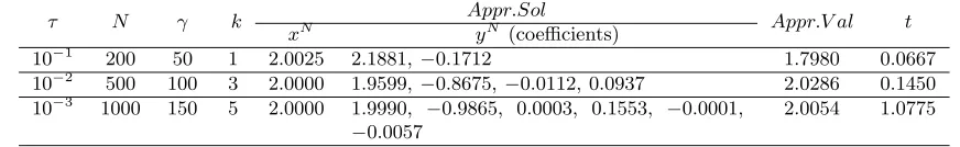
The numerical results are displayed in Tables 6.1 and 6.2. Here, τ denotes the regularization parameter, N the sample size, γ the parameter in entropy approximation,k the degree of the polynomial rule,Appr.Sol the approximate optimal solution and Appr.V al the optimal value, t the execution time (seconds). Note that

fmincon_{requires an initial point. We set the starting point to be a vector with components 1 for the entropic}

method and a vector with components 0 except the first component being 1 for Shapiro and Xu’s method.

Table 6.1

SAA-EA-PDL-RSMPEC scheme for problem (6.1)

τ N γ k Appr.Sol Appr.V al t

xN _yN _{(coefficients)}

10−1

200 50 1 2.0025 2.1881, −0.1712 1.7980 0.0667

10−2

500 100 3 2.0000 1.9599, −0.8675,−0.0112, 0.0937 2.0286 0.1450 10−3

1000 150 5 2.0000 1.9990, −0.9865, 0.0003, 0.1553, −0.0001,

−0.0057

2.0054 1.0775

Table 6.2

Shapiro and Xu’s method for problem (6.1)

τ N Appr.Sol Appr.V al t 10−1

200 1.0007 1.8752 0.7699

10−2

500 1.3159 2.1538 9.7875

10−3

1000 1.0023 1.8566 63.8623

Table 1 displays the results when the SAA-EA-PDL-RSMPEC scheme (4.6) is applied to problem (6.1). For the fixed regularization parameterτ = 10−1 _{and the sample sizeN = 200, the linear decision rule (k= 1)}

times is almost 60 times in favor of the decision rule. This is fundamentally due to the fact that under the decision rule approach, the number of constraints is independent of the sample size and hence the size of the resulting NLP is fixed. In contrast, Shapiro and Xu’s regularized SAA scheme does not enjoy this property. The difference of the optimal values is about 0.14 which means the SAA-EA-PDL-RSMPEC scheme (4.6) provides a reasonable upper bound for the problem. The preliminary tests results raises a promising prospect for the SAA-EA-PDL-RSMPEC scheme (4.6) although more numerical experiments are needed.

Next, we look into the EA-RMPDRE scheme (5.6).

Example 6.2. Consider the following mathematical program with distributionally robust equilibrium con-straints

min 100(x₋y) s.t. x∈[2,8],

EP[7 sinξ−x]≤0

0_≤y_⊥EP[(y+ sinξ−x)(x−2y)]≥0

∀P∈ P,

(6.2)

where_P :=_{Q_∈P:H(Q_|P0)≤c} andP0 ξ= iπ₈

= 1

5,fori= 0,1,2,3,4.It is easy to see that for each fixed

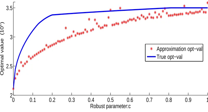
P ∈ P andx∈[2,8], both y=x/2 andy=EP[x−sinξ] satisfy the complementary constraint. However, here we require the complmentarity constraint to be held for all P _{∈ P}. This effectively excludes y =EP[x−sinξ] because it shifts asP varies. Therefore the set of feasible solutions to problem (6.2) is{(x, x/2) :x∈[u(c),8]}, where u(c) := maxP∈PEP[7 sinξ] is calculated from the inequality constraint. The objective function takes a value of 50xat the feasible solution point (x, x/2) and it is minimized at (u(c), u(c)/2) with the optimal value being50u(c).

0 0.1 0.2 0.3 0.4 0.5 0.6 0.7 0.8 0.9 1

2 2.5 3 3.5

Robust parameter:c

Optimal value (10

2 )

Approximation opt−val True opt−val

Fig. 6.1. Optimal value of problem (6.2)

We have carried out numerical tests on EA-RMPDRE scheme (5.6) by applying it to problem (6.2) with ambiguity parametercincreasing from 0 to 1. The red star dotted curve in Figure 1 displays the approximate optimal values obtained from solving the EA-RMPDRE scheme (5.6) withctaking values from 101 grid points evenly spread over the interval [0,1]. The blue curve corresponds to thetrueoptimal value 50u(c) whereu(c) is the optimal value of the following convex programming problem

min

P 50EP[−7 sinξ]

s.t. H(P|P0)≤c.

(6.3)

As it is too difficult to obtain a closed form for the optimal value of problem (6.3), we use solver CVX (version 1.2) developed by Michael Grant and Stephen Boyd [19] to solve for each fixedc.

The EA-RMPDRE scheme (5.6) is a nonlinear programming problem. We solve it with an exterior penalty function method and implement the latter through Matlab NLP solverfmincon3_{. As we can see from the Figure}

3

We set the maximal penalty parameter as 1000 and the tolerance as 10−3

1, the approximate optimal values obtained from latter fall below the true optimal values with a few exceptions. The underlying reason is that the regularization scheme and the penalty method enlarge the feasible set of the true problem and the “approximate optimal value” is obtained outside the feasible region. Asc increases, the ambiguity set gets larger and hence the set of feasible solutions to problem (5.6) becomes smaller. This explain the overall increasing tendency of the optimal values as c increases. We have also tested the impact of regularization parameterτ. It seems that reducing the value ofτ does not help to reduce the gap between the two curves. This is because the optimal solution obtained always satisfies the complementarity constraints (satisfyingy=x/2) in which case derivingτ to 0 does not help to reinforce the complementarity constraint.

Acknowledgements. We would like to thank the two referees and the Area Editor Mikhail V. Solodov for their constructive comments which significantly help us improve the presentation of the paper.

REFERENCES

[1] F. Alvarez and M. Carrasco, Minimization of the expected compliance as an alternative approach to multiload truss

optimization, Struct. Multidisc. Optim., 28 (2004), pp. 1-7.

[2] E. Anderson, H. Xu and D. Zhang, Approximating parametric maximization problems through CVaR with applications in minimax and robust convex optimization, manuscript, 2014.

[3] D. Az´e,A survey on error bounds for lower semicontinuous functions, ESAIM: Proc. 13 (2003), pp. 1-17.

[4] D. Bampou and D. Kuhn,Polynomial approximations for continuous linear programs, SIAM J. Optim., 22 (2012), pp. 628-648.

[5] A. Ben-Tal and A. Nemirovski,Robust truss topology design via semidefinite programming, SIAM J. Optim., 7 (1997), pp. 991-1016.

[6] A. Ben-Tal and A. Nemirovski,Robust convex optimization, Math. Oper. Res., 23 (1998), pp. 769-805.

[7] A. Ben-Tal and A. Nemirovski,Robust solutions of uncertain linear programs, Oper. Res. Lett., 25 (1999), pp. 1-13. [8] A. Ben-Tal, L. El Ghaoui and A. Nemirovski,Robust Optimization, Princeton University Press, Princeton, NJ, 2009. [9] A. Ben-Tal, A. Goryashko, E. Guslitzer and A. Nemirovski,Adjustable robust solutions of uncertain linear programs,

Math. Program., 99 (2004), pp. 351-376.

[10] A. Ben-Tal, D. Hertog, A.D. Waegenaere, B. Melenberg and G. Rennen,Robust solutions of optimization problems

affected by uncertain probabilities, Manage. Sci., 59 (2013), pp. 341-357.

[11] J. F. Bonnans and A. Shapiro,Perturbation Analysis of Optimization Problems, Springer Series in Operational Research, Springer, New York, 2000.

[12] G. Calafiore and M. C. Campi,Uncertain convex programs: randomized solutions and confidence levels, Math. Program., 102 (2005), pp. 25-46.

[13] G. Calafiore and M. C. Campi,The scenario approach to robust control design, IEEE Trans. Automatic Control, 51 (2006), pp. 742-753.

[14] G. Calafiore,Uncertain convex programs, SIAM J. Optim., 20 (2010), pp. 3427-3464.

[15] X. Chen, M. Sim, P. Sun and J. Zhang,A linear decision-based approximation approach to stochastic programming, Oper. Res., 56 (2008), pp. 344-357.

[16] E. Delage and Y. Ye, Distributionally robust optimization under moment uncertainty with application to data-driven

problems, Oper. Res., 58 (2010), pp. 595-612.

[17] H. F¨ollmer and A. Schied,Stochastic Finance: An Introduction in Discrete Time, Walter de Gruyter, Berlin, 2004. [18] H. F¨ollmer and T. Knispel,Entropic risk measures: coherence vs. convexity, model ambiguity, and robust large deviations,

Sto. Dynam., 11 (2011), pp. 333-351.

[19] M. Grant and S.Boyd, CVX, for convex optimization, download from the homepage http://www.stanford.edu/ boyd/. [20] J. Goh and M. Sim,Distributionally robust optimization and its tractable approximations, Oper. Res., 58 (2010), pp. 902-917. [21] Z. Hu and J. Hong, Kullback-Leibler divergence constrained distributionally robust optimization, manuscript, 2012. [22] D. Klatte,A note on quantitative stability results in nonlinear optimization, Seminarbericht Nr. 90, Sektion Mathematik,

Humboldt-Universit¨at zu Berlin, Berlin, pp. 77-86, 1987.

[23] D. Kuhn, W. Wiesemann and A. Georghiou,Primal and dual linear decision rules in stochastic and robust optimization, Math. Program., 130 (2011), pp. 177-209.

[24] G. H. Lin, X. Chen and M. Fukushima,Solving stochastic mathematical programs with equilibrium constraints via

approx-imation and smoothing implicit programming with penalization, Math. Program., 116 (2009), pp. 343-368.

[25] G. H. Lin and M. Fukushima, Stochastic equilibrium problems and stochastic mathematical programs with equilibrium

constraints: A survey, Pac. J. Optim., 6 (2010), pp. 455-482.

[26] Y. Liu, H. Xu and G. H. Lin, Stability analysis of two stage stochastic mathematical programs with complementarity

constraints via NLP-regularization, SIAM J. Optim., 21 (2011), pp. 609-705.

[27] Y. Liu, H. Xu and J. J. Ye,Penalized sample average approximation methods for stochastic mathematical programs with

complementarity constraints, Math. Oper. Res., 36 (2011), pp. 670-694.

[28] Z. Q. Luo, J. S. Pang and D. Ralph,Mathematical Programs with Equilibrium Constraints, Cambridge University Press, Cambridge, UK, 1996.

[29] F. Meng and H. Xu,A regularized sample average approximation method for stochastic mathematical programs with

nons-mooth equality constraints, SIAM J. Optim., 17 (2006), pp. 891-919.

[30] J. Outrata, M. Kocvara and J. Zowe,Nonsmooth Approach to Optimization Problems with Equilibrium Constraints:

Theory, Applications, and Numerical Results, Kluwer Academic Publishers, Dordrect, The Netherlands, 1998.

[31] J-S. Pang,Error bounds in mathematical programming, Math. Program., 79 (1997), pp. 299-332.

[32] M. Patriksson and L. Wynter,Stochastic mathematical programs with equilibrium constraints, Oper. Res. Lett., 25 (1999), pp. 159-167.