Incompressible SPH method based on Rankine source solution for violent water wave simulation

City, University of London Institutional Repository

Citation

: Zheng, X., Ma, Q. and Duan, W.Y. (2014). Incompressible SPH method based

This is the accepted version of the paper.

This version of the publication may differ from the final published

version.

Permanent repository link:

Link to published version

: http://dx.doi.org/10.1016/j.jcp.2014.07.036

Copyright and reuse:

City Research Online aims to make research

outputs of City, University of London available to a wider audience.

Copyright and Moral Rights remain with the author(s) and/or copyright

holders. URLs from City Research Online may be freely distributed and

linked to.

Incompressible SPH method based on Rankine source solution

for violent water wave simulation

X. Zheng1, Q.W. Ma2* , W.Y.Duan1

1. College of Shipbuilding Engineering, Harbin Engineering University, Harbin 150001, China 2. Schools of Engineering and Mathematical Science, City University London, London EC1V 0HB, UK

Abstract

With wide applications, the smoothed particle hydrodynamics method (abbreviated as SPH) has become an important numerical tool for solving complex flows, in particular those with a rapidly moving free surface. For such problems, the incompressible Smoothed Particle Hydrodynamics (ISPH) has been shown to yield better and more stable pressure time histories than the traditional SPH by many papers in literature. However, the existing ISPH method directly approximates the second order derivatives of the functions to be solved by using the Poisson equation. The order of accuracy of the method becomes low, especially when particles are distributed in a disorderly manner, which generally happens for modelling violent water waves. This paper introduces a new formulation using the Rankine source solution. In the new approach to the ISPH, the Poisson equation is first transformed into another form that does not include any derivative of the functions to be solved, and as a result, does not need to numerically approximate derivatives. The advantage of the new approach without need of numerical approximation of derivatives is obvious, potentially leading to a more robust numerical method. The newly formulated method is tested by simulating various water waves, and its convergent behaviours are numerically studied in this paper. Its results are compared with experimental data in some cases and reasonably good agreement is achieved. More importantly, numerical results clearly show that the newly developed method does need less number of particles and so less computational costs to achieve the similar level of accuracy, or to produce more accurate results with the same number of particles compared with the traditional SPH and existing ISPH when it is applied to modelling water waves.

Keywords: Meshless method; SPH; ISPH; ISPH_R; Free surface flow; Wave impact; Violent water waves

1. Introduction

Smoothed Particle Hydrodynamics (SPH) is a Lagrangian meshless particle method. It was originally developed to simulate astrodynamics [1, 2] but has been extended to model dynamics problems with violent motions in many areas [3-23]. The work on the method has been continuously reviewed by many authors. We mainly take some of these related to water wave modelling here.

When the SPH is applied to modelling water waves, there are largely two different formulations in literature. The first one is weakly compressible SPH (WCSPH, also called traditional SPH in this paper), in which water is considered as slightly compressible and its pressure is related to its density through an equation of state with artificially specified sound speed [6]. The second formulation is incompressible SPH, also called ISPH, in which water is considered as incompressible and having constant density with pressure found by solving a boundary value problem. As indicated by many researchers, e.g., Rafiee et al. [13] and Lee et al. [22], the WCSPH has several advantages, such as that it is easy to be programmed and does not need to solve pressure boundary value problem. However, it has at least two weaknesses [13, 22]: (a) requiring use of very small time steps and (b) resulting in significant spurious pressure fluctuations in space and time domain. The first one is inherent because the sound speed in the equation of state has to be large enough (even though much

*Manuscript

smaller than real sound speed), and so leads to smaller time steps. This is also related to that fact that the traditional SPH usually needs a large number of particles; in other words, very small distance between particles or very high resolution to obtain sufficiently accurate results. The more the particles in a given computational domain, the smaller the time steps should be used. The second weakness is perhaps because the pressure is very sensitive to the density and so a small error in density can lead to a significant error in pressure, inducing spurious pressure fluctuations. The spurious pressure fluctuations do not only give wrong values of pressure but can also cause simulation to become unstable when the method is employed to model wave-structure interactions. A great amount of effort has been made to overcome the weaknesses, for example, use of K2_SPH [8] and SPH based on the solution for Riemann problem [9-12]. K2_SPH improves the accuracy of kernel approximation for partial derivatives in continuity equation and momentum equations, and so can give more accurate results of density and velocity. In the SPH based on the solution for a Riemann problem, the Riemann problem is solved for each pair of particles to calculate the associated parameters. Basically, this approach improves accuracy of estimating the gradient involved. Its results are much more accurate and smoother than these from the traditional SPH, but it is significantly more expensive (in the order of 5 or 6 times) than the latter [13].

The ISPH has also been widely applied in the field of water wave dynamics [15-23]. This method projects the intermediate velocity field onto a divergence-free space by solving a Poisson equation for pressure. According to comparative studies carried out by Lee et al [22], the time step used for the ISPH can be much larger (50 times larger in one of cases presented by them). In addition, the results from ISPH can be much more accurate than these from the WCSPH for a given number of particles. In other words, the convergence rate of ISPH results is much higher than that of the WCSPH. The drawback of this formulation is obvious as it needs to solve the boundary value problem defined by the Poisson equation at each time step, which is recognised to consume a significant amount of computational time. Nevertheless, the total computational time taken by the ISPH can be shorter than that by the WCSPH, as indicated also by Lee et al. [22]. However, the second order derivatives of pressure need to be approximated when discretising the Poisson equation. In all publications found so far in literature about ISPH, the second derivatives are directly approximated using a scheme similar to that for finite difference method. No matter what scheme to be used, direct numerical approximation to second derivatives always has a difficulty with accurately modelling the functions to be solved, in particular when particles are distributed in a disorderly manner. Distribution of particles always becomes disorderly when modelling violent waves even they are regularly distributed at the start of simulation. Therefore, it is obviously advantageous to eliminate use of direct numerical approximation to second derivatives when solving the pressure Poisson equation in the ISPH formulation.

The distinct feature of this paper, compared with other papers on ISPH lies in that the pressure Poisson equation is first transformed into another equation based on a Rankine source solution using the same idea employed in Meshless Local Petrov-Galerkin Method based on Rankine Source Solution (MLPG_R) [24-30]. In the new formulation of ISPH, the governing equation for pressure does not include any derivatives of the functions to be solved and so overcomes the problems associated with direct numerical approximation to second derivatives in existing ISPH formulation. This new formulated ISPH is named as ISPH_R for convenience in this paper. According to our benchmark tests presented in this paper below, the ISPH_R method can give more accurate results and consume less computational time when modelling water waves.

2. Governing equations and numerical schemes

2.1. Traditional SPH method

The formulation of the traditional SPH can be found in many publications but it will be outlined in this section for completeness. The method is generally based on the Lagrangian form of continuity equation and the Navier-Stokes equation for compressible flow, which may be written as

0

D D

˜ ’ U u

U

u 1 g 2u D D ’ ’ Q U p

t (2)

whereU is the fluid density, uis the fluid velocity, tis the time, p is the fluid pressure, gis the

gravitational acceleration, and Q is the kinematic viscosity. In WCSPH, the pressure and density are usually

related by the following equation of state for sound waves

] 1 ) [( 0 0 2 0 N U U N U c

p or p c₀2(UU₀) (3)

where N 7 is used for liquid water simulation, c₀is the artificial sound speed and usually chosen as 10

times of maximum fluid velocity, U₀is the initial density of water. In the SPH formulation (see for example,

Monaghan, 2005 [23]), the pressure gradient and velocity divergence may be estimated, respectively, by

’ |

¦

2 ) ( )

( r

U U

U (4a)

’˜ |

¦

i m W

1

) (

1 _{u r}

u

U (4b)

where u_ij u_iu_j, m_jis the mass bearded by particle j and Wis a kernel function. There are many

forms of the kernel function. The one used in this paper is given by

° ° ° ° ¯ °° ° ° ® ­ ! d d 2 0 2 1 ) 2 ( 6 1 1 0 ) ( 2 1 ) ( 3 2 ) ( 3 3 2 h h h h h h W j i j i j i j i j i j i d ij r r r r r r r r r r r r

r _D (5)

where h is equal to 1.8s (s is the initial distance between particles) in this paper and Dd is taken as

15/(7*S*h2) in 2D cases. Using Eq. (4), the velocity and density of each particle may be updated by the

following equations:

u |

¦

N j ij ij j j i i j

i _m p p _W

Dt D

1

2

2 ) ( )

(

U

U (6)

|

¦

i m _W

Dt D 1 ) (r u U U

U ₍₇₎

° ¯ ° ® ­ t ˜ ˜ – 0 0 0 ~ ~ 2 0 ij ij ij ij ij ij ij ij c r u r u U P [ P Z (8)

where the artificial viscosity is given by _{2 2}

01 . 0 ~ h h ij ij ij ij ˜ r r u

P , r_ij r_i r_j, Uij (Ui Uj)/2. The value of

Z and [ in Eq. (8) is constant and is problem-dependent, which are taken as Z 0.3 and [ 0 _{in this}

velocity, Monaghan [6] suggested the following equation for calculating positions

|

¦

N j

ij ij j j

i W

m Dt

D

1

) (r

u u

x_i

U

H (9)

where H _{is a constant in the range of} 0dH d1. In this paper, H 0.01.

2.2. ISPH method

In the incompressible SPH method, the fluid density is considered as a constant, and as a result, the continuity equation can be written as

0 /Dt

DU (10a)

or

0

˜

’ u (10b)

The momentum equation remains the same as in Eq. (2). The computation in the ISPH method is composed of two basic steps, following the procedure in [41]. The first step is a prediction, in which the velocity field is computed without imposing incompressibility. The second step is a correction in which incompressibility is enforced, leading to the Poisson equation for solving pressure. More details can be found in, e.g., Shao et al. [17]. Summary will be given below.

(a) Prediction step

Assuming that velocities and positions of particles at time t have been found, their velocities and

positions at t't are first predicted by considering gravitational term and viscous term in Eq. (2) using

the following equations,

u_* u_t'u_* (11)

t ' ’

' ( 2 )

* g u

u _Q (12)

t

t *'

* r u

r (13)

where u_t and r_t are the velocities and positions at time t, respectively; 't is the time step; r_* and

*

u

' are the predicted intermediate position and velocity of particles at the new time step.

(b) Correction step

The velocity change during the correction step is estimated by

't’p_t't

U

* *

u (14)

where p_t't is the pressure at t't. The velocities and positions of particles at t't are then given by u_t't u_* u_** (15)

t t t t

t t

t '

'

'

2

u u r

r (16)

Combining Eq. (10b) with Eq.(14), one obtains the following equation for pressure

t p_{t t}

' ˜ ’

’2 ' *

u

U ₍₁₇₎

2 *

* )

1 (

t p_{t t}

' ’

˜

’ _U ' U_U U (18)

where U* is the density at the intermediate time step and can be estimated by

¦

N j

ij jW

m

, 1 *

U . For the

incompressible fluids, the intermediate density is not much different from the specified fluid density. As indicated by Hu and Adams [19], Eq. (17) and (18) are equivalent and both valid for incompressible fluids theoretically. They suggested solving the two incompressibility equations simultaneously. The solution of the density invariant equation (Eq. 18) was used to adjust the positions of particles while the solution of the velocity-divergence-free equation (Eq. 17) was used to adjust their velocity. In contrast, Zhang et al [43] proposed using the mixed one given below

pt t _{t 't}

˜ ’ '

’ ' 2 *

* 2

) 1

( J U u

U U

J (19)

which was also used by Ma et al. [26] for the MLPG_R method, where J is the artificial value and in the

range of 0- 1. According to numerical tests presented in Ma and Zhou [26] and also suggested by Zhang et

al [43], the results for violent water waves obtained by using Eq. (19) seems to be better if J is specified a

proper small value than those for J 0(velocity-divergence-free equation). In order to achieve good

results without need of the density term (i.e. J 0), the position of particles may be shifted at each time

step in a way similar to remeshing or dynamic regridding, such as that based on the Fick’s law employed by Lind et al [21], or that according to the velocity calculated from pressure gradients relative to a minimum pressure proposed by Sriram and Ma [28]. These techniques had been found to make the distribution of particles significantly more regular and lead to much better results compared with these from using either Eq. (17) or Eq. (18) separately. Xu et al [44] compared four methods (two of them are based on Eq. (17) and Eq. (18), respectively; the third one is the approach of Hu and Adams [19] and the fourth one is based on the approach of shifting the positions of particles they proposed). They concluded that the approach of using only Eq. (17) may exhibit instability in some cases, the one with Eq. (18) may overcome the instability caused by ill-distributed particles but was shown giving inaccurate predictions with extremely high noise in results, and the particle shifting technique can help achieving accurate and stable simulations as the approach of Hu and Adams [19] does but needs much less computational time than the latter. Such comparative studies are not the focus of this paper, though the studies may be necessary to judge if the approach based on Eq. (19) and the one proposed by [28] could be as good as the particle shifting technique and the approach of Hu and Adams [19] in the same cases. Based on our experience in modelling violent water waves, we choose in this paper to use Eq. (19) which does not need extra computation related to

shifting particles but we accept the possibility that combining the particle shifting technique with the new

technique for solving the pressure Poisson introduced in the paper may give better results than these

presented in the current paper. For solving the pressure Poisson equation (either Eq. 17, Eq. 18 or Eq. 19 ),

several different discretised schemes of the Laplacian operator have been suggested previously but the often employed scheme (e.g., [4],[16] and [22]) is the one given below:

¦

|

’ N

j

ij ij

ij ij

j j

i p

r W m

p

1

2 2

,

2 ₂ ( )

G U

D D r r

(20a)

where p_ij (p_i p_j), subscript denotes the direction and corresponds to x and y in two-dimensional (2D)

cases, W(r_ij)_,Dis the partial derivative of the kernel function with respect to the coordinate in direction,

D

ij

r is the component of the vector r_ij in direction, _D

D ( ij),

ij W r

r is r_ij ˜’W(r_ij). These explanations

It has been well known that the discretised Laplace operator given by Eq. (20a) may produce large errors in particular when the particles are distributed in a disorderly manner as happen in violent water wave problems. To improve the accuracy of the discretised Laplace operator, Schwaiger [39] proposed several forms of a higher order method for Laplace operator discretisation. Two of them are based on the following equation °¿ ° ¾ ½ °¯ ° ® ­ ˜ | ’

¦

¦

p D D _{D D}

U U

EE r r _r

(20b)

where is a tensor that is defined as

³

:i ij ij ij ij j j W m

_EF D D _{E F}

U r r r

r

2 ,

, n is the number of dimension (n=2

for 2D cases), D andE denote different directions and correspond to x and y in 2D cases. The difference

between the two forms of the high order Laplace operator discretisation lies in how to estimate the gradient

in the second term of the right hand of Eq. (20b). In one form, the gradient in the term is estimated by

¦

i p p W

m p

1

,

,D ( ) D

U (20c),

while in the other form, the gradient is estimated by

¦

i p p L W

m p

1

,

,D ( ) DE E

U (20d)

where 1 , , , 1 ) ( ¸¸¹ · ¨¨© §

¦

DE _U x x W

m

L _{j i}

N j j

j

, which is an inverse matrix.

In Schwaiger [39], the method based on Eq. (20b) and Eq. (20c) was called as SPH2, while the method based on Eq. (20b) and Eq. (20c) is called as CSPH2. They also suggested another method based on solving all the second order derivatives and named it as CSPM. Schwaiger [39] compared the convergence properties of all the forms including the three methods (SPH2, CSPH2 and CSPM) by applying them to estimate the second order derivatives on a set of particles distributed in a disorderly manner. They demonstrated that their CSPH2 and CSPM methods have similar convergence properties, but the CSPM method is expected to take much more CPU time. Lind et al [21] applied the CSPH2 method to study water wave problems, and indicated that it can give better results by combining it with a particle-shifting technique they suggested. Fatehi and Manzari [40] also suggested a high order method for Laplace operator discretisation, which is similar to the CSPM method in the sense that both need to solve all the second order derivatives.

In this paper, we will compare several forms of ISPH methods with our proposed method. The different forms of the methods used are defined as below:

1) SPH: tradional SPH as discussed in Section 2.1 2) ISPH - incompresible SPH based on Eq. (20a)

Although Schwaiger [39] and Lind et al [21] had carried out patch tests by applying Eq. (20b) to estimate the second order derivatives of the several functions on a set of particles distributed in a disorderly manner, more tests will be carried out in this section to further show the behaviours of ISPH, CISPH1 and CISPH2, in particular when the disorderliness of particle distribution varies.

For this purpose, we will consider the function of f(x,y)=cos(4x+ 8y). The space domain is chosen as a square with the length of sides 1 for 2 x 3 and 2 y 3. The domain is first divided into small squared elements ( 'xu'y with 'x 'y s ). The particles are then redistributed according to

)] 5 . 0 ( 1

[

c ' c

'x y s k Rn , where Rnis a random number between 0 and 1.0 and k is a constant that can be taken as a value between 0 and 1. Clearly, k=0 leads to regular distribution of particles. k>0 makes the distribution of particles become disorderly. As k increases, the distribution is more disorderly. The Laplacian of f(x,y) is calculated by directly taking mathematical derivatives, which is denoted as ’2f_i,a, and estimated numerically by using the three methods mentioned in the previous paragraph, which is denoted as

c i

f_,

2

’ . The accuracy of the numerical methods is quantified, in a similar way to that used in Schwaiger [39], by evaluating their average relative errors given as

¦

i i

i m

a i

a i c

i m

f f f

Er

1

2

, , 2

, 2 , 2

) (

U ,

where ’2f_i,a,m is the magnitude of ’2f_i,a , e.g., ’2f_i,a,m 80S2 , for f(x,y)=cos(4x+ 8y). When estimating the error using the above equation, only the particles within the region of 2.2dxd2.8

8 . 2 2

.

2 d yd are considered. The accuracy of the methods is also quantified by estimating their maximum relative errors given as

N i

f f f

Er

m a i

a i c

i

3 , 2 , 1 ), max(

, , 2

, 2 , 2

max

’ ’ ’

- 2. 2 - 2. 0 - 1. 8 - 1. 6 - 1. 4 - 1. 2 - 1. 0

- 1. 5 - 1. 4 - 1. 3 - 1. 2 - 1. 1 - 1. 0 - 0. 9 - 0. 8 - 0. 7 - 0. 6 - 0. 5 - 0. 4 - 0. 3

lo

g

(

E

r

)

l og( s )

I SPH CI SPH1 CI SPH2

- 2. 2 - 2. 0 - 1. 8 - 1. 6 - 1. 4 - 1. 2 - 1. 0

- 0. 6 - 0. 4 - 0. 2 0. 0 0. 2 0. 4 0. 6

lo

g

(

E

r

m

a

x

)

l og( s )

I SPH CI SPH1 CI SPH2

(a) (b)

Fig. 1 Relative errors of different discretised Laplace operators for different values of s with the value of k fixed to be 0.8 (a) average error; (b) maximum error.

average error of CISPH2 is consistently reduced with reduction of s while it was shown to remain to be constant in Schwaiger [39] for a function of x2+y2. The averages errors of other two methods can increase with the reduction of s, which is a divergent behaviour. The behaviour of ISPH is similar to what was shown in Schwaiger [39] but the behaviour of CISPH1 is slightly different as they showed that its average error remained as constant. The results of maximum error given in Fig. 1(b) demonstrate that the error of all three methods can increase with increasing the resolution of the particles. In addition, the smallest value of the error is Log(Ermax)>-0.6, corresponding to Ermax =25%, which is considerably larger than the value of

average error for the same case.

0. 0 0. 2 0. 4 0. 6 0. 8 1. 0 1. 2 - 2. 5

- 2. 0 - 1. 5 - 1. 0 - 0. 5 0. 0

lo

g

(

E

r

)

k I SPH CI SPH1 CI SPH2

0. 0 0. 2 0. 4 0. 6 0. 8 1. 0 1. 2 - 2. 0

- 1. 5 - 1. 0 - 0. 5 0. 0 0. 5 1. 0

l

o

g(

Er

m

a

x

)

k I SPH CI SPH1 CI SPH2

(a) (b)

Fig. 2 Relative errors of different discretised Laplace operators for different values of k with the value of s fixed to be 0.01 (a) average error; (b) maximum error.

20 30 40 50 60 70 80 90 100

0 50 100 150 200 250 300 350 400 450 500 550

P

a

r

t

ic

le

n

u

m

b

e

r

s

Er i ( %)

I SPH CSPH1 CSPH2

Fig. 3. Number of particles with a large relative error (>20%) for s=0.01 and k=1.2

Fig. 2 plots the average and maximum errors for different values of k with s=0.01. One can see from the figures that the errors of the three methods increase with the increase of k values, i.e., with particle being more disorderly. Furthermore, the maximum error can be become very large, for example, Log(Ermax)>-0.25, corresponding to Ermax = 56%, at k=1.2. It is noted that overall accuracy of numerical

In Fig. 3, the horizontal axis shows the different ranges of relative error, e.g., [10%, 20%] and [20%, 30%], while the vertical axis shows the number of particles whose error lies in a range. For example, in the range of [10%, 20%], there are about 550 particles for the CISPH1 method and about 225 particles for the CISPH2 method. The relative error at each individual particle used in this figure is defined as

) 3 , 2 , 1 (

, , 2

, 2 , 2

N i

f f f

Er

m a i

a i c i

i

’ ’ ’

. This figure demonstrates that the quite large relative error (>20%)

can happen at a considerable number of particles for all the three methods even when they are applied to computing the Laplacian of the quite simple function, though the number for the CISPH1 and CISPH2 method is smaller than for ISPH method.

These results demonstrate that although a lot of effort has been made to develop the approximations to the Laplacian operator discretisation, it still needs to be improved in particular for modelling violent water waves where the particles can become severely disordered without regularisation by shifting even they are uniformly distributed at the start of simulation. The new approach suggested below is to overcome the weakness associated with discretisation of Laplacian operator in the ISPH method.

2.3. ISPH_R method

The main difference between the existing ISPH method and the new method named as ISPH_R method lies in the approach to discretisation of the pressure Poisson equation defined in Eq. (19). The main idea of the new approach comes from another meshless method called as the Meshless Local Petrov-Galerkin Method based on Rankine Source Solution (MLPG_R) [25][26], that is, reformulating Eq. (19) into another form which does not include any derivative of pressure and velocity. For this purpose, Eq. (19) is integrated over a small sub-domain :_I(to be distinctive, notation of particles for the ISPH_R method is denoted by capital I or J) surrounding a particle after multiplication by the Rankine source solution M, and then it reads

³

³

:

'

: _{' '} ’˜ :

’

I I

I I

t

t d

t t

d

p J U U J U M

M [ 2 (1 ) *]

*

2 _{u (21)}

where M can be chosen as

) / ln( 2

1

I

R r S

M for 2D cases (22)

that satisfies ’2M 0, in :_I except for the center and M 0, on w:_I, which is the boundary of :_I and R_Iis its radius. The radius is usually smaller than the distance between two particles. After some mathematical manipulations, Eq.(21) becomes the following form

' '

’

˜

_³

³

: w

' '

d

t R

t p

dS p

I I

I I I I t t t

t M

U J U

U J

M *

2

2 *

) 1 ( 4 )

( u

n& (23)

which will be applied to each of inner particles. More details of mathematical manipulations can be found in Ma and Zhou [26]. It has been noted that the increment of the density (UU*) assumed to a constant within the sub-domain and so equal to its value at Particle I when Eq. (23) is derived. This may not cause unacceptable error not only because the density should not change much due to the change in the intermediate position of the particle as pointed above but also because the small error caused due to the assumption is further reduced by multiplying the coefficient J _{that is normally chosen in a range of 0~0.3,} taken as 0.1 in this paper. The term may be evaluated in the same way as that for the second term but such a way will not improve the accuracy significantly due to the reasons discussed here.

functions to be solved while Eq. (19) contains the second order derivative of pressure and the first-order derivative of velocity. Approximation to the functions in Eq. (23) does not require them to have any continuous derivatives, while approximation to the functions in Eq. (19) requires them to have finite, or at least integrable second order derivatives. Therefore, use of Eq. (23) for further discretisation has a great numerical advantage over use of Eq. (19) directly, and so potentially makes the ISPH_R more accurate for the same number of particles or require less number of particles to obtain the solution with the same order of accuracy than ISPH, which will be demonstrated in the later sections of this paper.

2.4. Boundary conditions

Generally, there are two kinds of boundary conditions for water wave problems. One is on solitary boundaries and one on the free surface. They are outlined separately below.

2.4.1. Solid boundary conditions

On solid boundaries, the following conditions (e.g. Ma and Zhou [26] or Sriram and Ma [28]) should be satisfied

n U n

u_{˜ ˜} (24)

and

n_˜’ U _{˜ ˜} Q _˜’2

p

(25) where n _{is the unit normal vector of the solid boundaries,} gis the vector of gravitational acceleration,

UandU are the velocity and acceleration of the solid boundaries, respectively. It is noted that the traditional SPH does not need the condition in Eq. (25) as it does not need to solve the boundary value problem for pressure. In the ISPH method, the condition in Eq. (25) is necessary.

It is obvious that one must compute the term ’2u when applying this condition in Eq. (25), which needs to estimate the second order derivative at the rigid boundary. To avoid the computation of the second order derivative in the equation, Ma and Zhou [26] combined Eqs. (11) with (25) and gave an alternative as follows:

) (u* U

n

n ˜

' ’ ˜

t p U

(26)

This one is used in this paper.

Numerical implementation of Eq. (24) is relatively straightforward, i.e., the normal velocity of fluid particles is imposed to be equal to the normal velocity of wall that is given in the cases of this paper. Numerical implementation of Eq. (26) is different for different SPH methods described above. For the traditional SPH, there is no need to solve the Poisson's equation (Eq. (19)) for pressure and so it is not necessary to use this equation. However, in order to improve the computation of pressure gradients in Eq. (4a) for updating the velocity, the two-layer ghost particles are adopted as described, such as in [22]. For ISPH and ISPH_R methods, Eq. (26) is discretised at the points on solid boundaries, in which the normal gradient of pressure is estimated at the boundaries without the assistance of any ghost particles by using the following equations

¦

˜ N

J

J IJ r p r

p I

1

& &

&

n

where <IJis defined by Eq. (A6) in Appendix A. It is noted that Eq. (26b) is based on the approximation

form used in this paper is slightly different from that given in Ma (2007), in the sense that the expression of

IJ

< is directly given here.

2.4.2. Free surface condition and Free surface particle identification

The condition on the free surface is very simple, which is stated that the pressure of water on its free surface is equal to the atmospheric pressure which can be taken as zero, i.e.,

0

p (27) In the traditional SPH method, this condition is automatically satisfied as long as the density on the free surface is estimated correctly, as one would see in Eq. (3). However, in the ISPH method, this condition has to be imposed when solving the boundary value problem defined by Eqs. (17), (18), (19) or (23). In order to impose this condition, one needs to know which particles are on the free surface. This is not a problem for non-broken water waves, where the water particles on the free surface at start always remain on the free surface and does not need to be identified during simulation. However, for breaking or violent water waves, the particles on the free surface at start can become inner particles and inner particles can become the free surface particles during a simulation. Therefore, the free surface particles have to be identified at every time step after wave breaking occurs. Many publications (e.g., Shao et al. [18]) on the ISPH method use the ratio

of

0

U U

D I

I , where UIis estimated by |

¦

IJ J I m W

, 1

U , to identify the free surface particles but often shows

wrong identification. A number of researchers have tried to address the inaccuracy of the approach based

only on

0

U U

D I

I , for example, Lee at el [22] employed the gradient of position vector,׏ ȉ ࢘, to judge if a

particle is on the free surface (ȁ׏ ȉ ࢘ȁ ൏ ͳǤͷ) or not. However as indicated by Lind et al [21], some internal fluid particles may satisfyȁ׏ ȉ ࢘ȁ ൏ ͳǤͷ, while some free-surface particles may ȁ׏ ȉ ࢘ȁ ൐ ͳǤͷ, leading to misjudgement. Another method has been recently proposed for the SPH method by Zheng et al. [32]. For completeness, this method is summarised here and more details can be found in Zheng et al. [32]. The main idea of the method is to define three auxiliary functions on the influence domain around a particle, as shown in Fig. 4. The influence domain is determined by the kernel function, i.e., the kernel function at particle I is zero outside the influence domain. The influence domain is divided into four parts in two different ways, as seen in Fig. 4. One way is that it is divided into four quadrants by x- and y- axes and the other is divided into four shaded areas. The angle of each shaded part covers an area of 90 degrees, and is symmetrical to the xor the

yaxis, respectively. The first auxiliary function is defined as

¯ ®

­ t

0 0

1 1

) ( _

NumA NumA I

a

fsp (28)

where NumA represents the number of free surface particles existing in the influence domain of Particle I _in previous time step. The value of NumA is equal to or larger than 1 if there is any neighbour free surface particle in the influence domain in Fig. 4; otherwise it is zero. The second auxiliary function is

¯ ® ­

d3 0

4 1

) ( _

NumB NumB I

b

fsp (29) where NumB represents the number of quadrants of the influence domain occupied by the particles in a local coordinate system centred at Particle I. NumB 4if all the 4 parts in Fig.4a have neighbour particles and

3

function is given by

¯ ® ­

d3 0

4 1

) ( _

NumC NumC I

c

fsp (30) where NumC represents the number of shaded parts of the influence domain containing at least one fluid particle. If all the 4 shaded parts in Fig.4b have neighbour particles, then NumC=4. Similarly, if 3 shaded parts in Fig.4b have neighbour particles, NumC=3. At each time step, each of potential free surface particles is checked in the following sequence:

(a) No inner particle in the influence domain except for Particle I (b)D_I d0.90 and fsp_a(I) 1

(c)D_I !0.90, fsp_a(I) 1 and fsp_b(I) 0 (d) D_I !0.90, fsp_a(I) 1 and fsp_c(I) 0 (e) D_I d0.90,NumBd2 and NumC d2

If any of expressions is true during checking, Particle I is identified as a free surface particle. The group of potential free surface particles is selected according to the free surface particles and their neighbours in previous two time steps. In the sense that only the potential free surface particles, not all, are checked, the aspect of the method is similar to what was suggested by Marrone et al [41].

As tested by Zheng et al. [32], this technique can give significant improvement on identifying the particles on the free surface, as shown in Fig. 5. The left one shows the configuration of particles at a time instant with the free surface particles (blue dots) identified by only using the ratio (D_I 0.9) of the density while the right one shows that with the free surface particles (blue dots) identified by using the above method. It can be seen that many inner particles are identified as the free surface particles by the method based only on the density ratio while the method described above can correctly identify almost of them on and near the free surface. It is noted nevertheless that a few particles near the free surface may still be identified as free surface particles but such incorrect identification may not lead to significant error on pressure. That is because the pressures of these particles are very close to the pressure on the free surface. More details of verification and comparison is referred to Zheng et al. [32].

x y

i

(a) (b)

Fig. 4 Illustration of influence domain and its divisions

x y

(a)based on density ratio only (b) Method of Zheng et al. [32]

Fig. 5 Comparison of free surface particle identification methods (blue dotes: free surface particles; red dots: inner particle)

2.5. Discretisation of pressure governing equation for ISPH and ISPH_R methods

As has been indicated above, the ISPH and ISPH_R methods require solving the boundary value problem for pressure defined by Eqs. (19) or (23), (26) and (27) at each time step. For this purpose, they must be discretised by using a set of particles to form the following algebraic system.

B P

A_˜ (31)

where P is a column vector formed by the pressure, A and B are the matrices. The specific expressions of entries in A and B depend on the scheme for discretising the governing equations. For the ISPH method, if one uses Eq. (20a) to discretise the Laplace operator at inner particles and Eq. (26b) to discretise the boundary condition on the solid boundaries, the expressions of entries in A and B are given by

° ¯ ° ® ­

¦

boundaries solid

on particles for

particles inner

for 2

1

2 2

,

IJ N

J IJ IJ J J

IJ r

W r m A

<

G U

D D

(32a)

° ° ¯ ° ° ® ­

»¼ º «¬

ª _˜

» ¼ º «

¬

ª ’˜

_{) forsolidboundaryparticles}

(

particles inner

for )

1 (

1 *

* 2

*

I n

I I

t

t t

B

U u n

u

'U

' U D ' U

U D

(32b)

Similar expressions can be written out if one employs Eq. (20b) to discretise the Laplace operator at inner particles but details are omitted here.

For the ISPH_R method, the pressure in Eq. (23) is approximated by |

¦

N j

j j x p

x

p

1

&

& _{at all inner}

particles, where _j x& is the shape function which may be formulated by using the moving least square method (MLS) as in [24-26], or the interpolation scheme developed by Ma [29]. In this paper, the MLS is used. The details about formulating the shape function can be found in Ma [24], and so will not be given here. With the approximation to pressure and after converting Eq. (23) and (26) into Eq. (31), the entries of

A and B are given, respectively, by

x

y

0

1

2

3

4

5

1

2

3

x

y

0

1

2

3

4

5

°¯ ° ®

­

_³

w

nodes boundary solid

for

nodes inner for )

( )

(

IJ

I J

IJ I

x ds

n x A

<

) M )

:

& &

&

(33a)

° ° ¯ °° ® ­

˜

’ ˜

³

nodes boundary solid

for )

(

nodes inner for )

1 ( 4

1

* 2

2 *

n I I I I

t

d u

t R

t

B I

U u n& &_* &

&

'U

: M 'U

D ' U

U D

:

(33b)

When forming the above equations, the pressure at the free surface particles has been imposed to be zero, according to Eq. (27). In Eq. (33), one needs to evaluate the integrals at each particle over its sub-domain. This potentially takes significant computational time but the semi-analytical technique suggested by Zhou and Ma [27] helps reducing the costs considerably and is adopted in this paper.

3. Numerical tests, validation and discussions

In this part, the method described above will be tested for the several water wave problems and also for lid-driven flow, and validated by comparing its results with those in literature. Its behaviours will also be compared with the traditional SPH and different forms of existing ISPH methods in the cases for water waves.

3.1. Dam breaking flow

D L

H

P1 P2

h1 h2

Fig. 6 Sketch of dam breaking flow

Dam breaking is often used as a benchmark for violent free surface flow. In this numerical test, a rectangular water column is confined between bottom, top wall and two vertical walls, as illustrated in Fig. 6. The width of the water column is L and its height is H. At the beginning of the computation, the dam is instantaneously removed and the water collapses and flows out along a dry horizontal bed. D _{is the} distance between two vertical walls. There are two pressure sensors p₁ and p₂ on the left and right vertical walls, respectively. The height of p₁ and p₂ from the bottom is h₁ and h_{2 respectively. In this} section, all variables and parameters are non-dimensionalised using H _and g, such as ~t t g/H unless mentioned otherwise.

3.1.1. Dam breaking flow with non-breaking waves

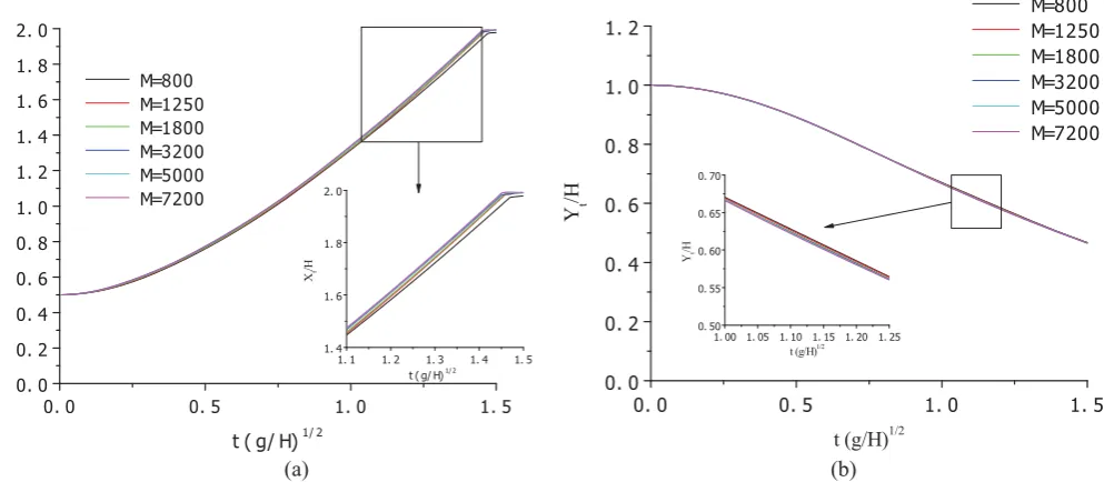
developed for modelling the violent breaking waves, it is used here for preliminary validation of the method. That is because the error could be estimated precisely against the experimental data in such a case. For this purpose, the parameters in Fig. 6 are taken as L=0.5m, H/L 2.0 and D/L 4.0, and the number of participles is chosen to be M 800, 1250 1800, 3200, 5000, 7200, corresponding to s 0.025, 0.02, 0.0167, 0.0125, 0.01, 0.00833, respectively. The time step length is selected as '~t 0.008. The time histories of the water front (Xf) and the water column height (Yt) at the left vertical wall after collapsing of

the water column corresponding to different numbers of particles obtained by using the ISPH_R are plotted in Fig. 7. It can be seen that the results are very close to each other, which indicates that 800 particles can lead to sufficiently accurate results in this case. Fig. 8 gives the results of water front and water column height at the left vertical wall obtained by using the ISPH_R method, all three forms of ISPH method and traditional SPH described above and their comparison with published experimental results [33]. According to the results in Fig. 8(a), the water front results obtained by ISPH_R and two SPH methods agree quite well with experimental results, though there are visible differences between the computational and experimental results. However, the results are very close to the results obtained by using MAC [34]and VOF [35] methods. From Fig. 8(b), one may observe that the results of water column height at the left vertical wall from all the methods (ISPH_R, CISPH2 and SPH) do not have much difference with experimental results.

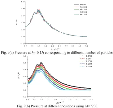
The time histories of pressure recorded at h₁ 0.1H corresponding to different particle numbers are presented in Fig. 9(a), which are computed by using the ISPH_R method. It can be seen that when the number of particles is not large enough, such as M 800, there are some spurious fluctuations in the pressure time histories, while they can be suppressed with increase of particle numbers, for example,

3200

!

M in this case. This case indicates that spurious fluctuations in the pressure results computed by the new developed ISPH_R method become insignificant when the particle number is large enough, similar to the features of the existing ISPH method as indicated by Lee et al. [22] where the results of the SPH were shown to have large fluctuations. Fig. 9(b) compares the results corresponding to the different values of h₁ of Point p₁ with M 7200, i.e., h₁ 0.05H,0.1H,0.15H,0.20Hand0.25H. One can see from this figure that all the pressure time histories are quite smooth.

0. 0 0. 5 1. 0 1. 5 0. 0

0. 2 0. 4 0. 6 0. 8 1. 0 1. 2 1. 4 1. 6 1. 8 2. 0

1. 1 1. 2 1. 3 1. 4 1. 5 1. 4

1. 6 1. 8 2. 0

Xf

/H

t ( g/ H)1/ 2

Xf

/H

t ( g/ H)1/ 2

M=800 M=1250 M=1800 M=3200 M=5000 M=7200

0. 0 0. 5 1. 0 1. 5

0. 0 0. 2 0. 4 0. 6 0. 8 1. 0 1. 2

1. 00 1. 05 1. 10 1. 15 1. 20 1. 25 0. 50

0. 55 0. 60 0. 65 0. 70

Yt

/H

t (g/H)1/2

Yt

/H

t (g/H)1/2

M=800 M=1250 M=1800 M=3200 M=5000 M=7200

(a) (b)

Fig. 7 Comparison of (a) water fronts represented by Xf and (b) water column heights represented by Yt

0. 0 0. 5 1. 0 1. 5 0. 0

0. 5 1. 0 1. 5 2. 0 2. 5

Xf

/H

t ( g/ H)1/ 2

Exp[33] MAC VOF SPH ISPH CISPH2 ISPH_R

0. 0 0. 5 1. 0 1. 5 0. 0

0. 2 0. 4 0. 6 0. 8 1. 0 1. 2

Yt

/H

t ( g/ H)1/ 2

Ex p[ 33] SPH I SPH CI SPH2 I SPH_R

(a) (b)

Fig. 8 Comparison of water fronts (a) and water column heights (b) with experimental data [33] when

7200

M

0. 0 0. 5 1. 0 1. 5 2. 0 2. 5 3. 0 3. 5 4. 0 4. 5 - 0. 2

0. 0 0. 2 0. 4 0. 6 0. 8 1. 0

p/

U

gH

t ( g/ H)1/ 2

M=800 M=1800 M=3200 M=5000 M=7200

Fig. 9(a) Pressure at h1=0.1H corresponding to different number of particles

0. 0 0. 5 1. 0 1. 5 2. 0 2. 5 3. 0 3. 5 4. 0 4. 5 - 0. 2

0. 0 0. 2 0. 4 0. 6 0. 8 1. 0

p/

U

gH

t ( g/ H)1/ 2

0. 05H 0. 1H 0. 15H 0. 20H 0. 25H

Fig. 9(b) Pressure at different positions using M=7200

Fig. 9 Time histories of pressure computed by using ISPH_R method

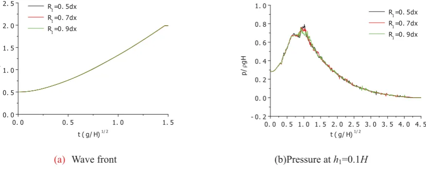
Another issue is also addressed by using the above case, which is about the size (RI) of the integration

domain (:_I) related to Eq. (23) for the ISPH_R method. It is noted that Eq. (23) is similar to that for MLPG_R method [24-30] as mentioned before. The effects of RI have been discussed, for example, by Ma et

al [25], which showed that RI could be selected in the range of 0.3 to 0.9 dx (dx here is the minimum distance

The corresponding results of the wave front and pressure at h1=0.1H are plotted in Fig. 10. It can be

observed that there is no visible difference in Fig. 10(a) while very small one in Fig. 10(b). RI = 0.5dx are

used for the cases in this paper.

0. 0 0. 5 1. 0 1. 5

0. 0 0. 5 1. 0 1. 5 2. 0 2. 5

Xf

/H

t ( g/ H)1/ 2

R_I=0. 5dx R_I=0. 7dx R

I=0. 9dx

0. 0 0. 5 1. 0 1. 5 2. 0 2. 5 3. 0 3. 5 4. 0 4. 5 - 0. 2

0. 0 0. 2 0. 4 0. 6 0. 8 1. 0

p/

U

gH

t ( g/ H)1/ 2

R_I=0. 5dx

R_I=0. 7dx

R_I=0. 9dx

(a) Wave front (b)Pressure at h1=0.1H

Fig. 10 Effects of different sizes (RI) of the integration domain in ISPH_R method (M 7200)

3.1.2 Dam breaking flow with breaking waves

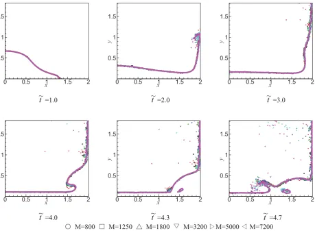
It is more important to consider the dam breaking flow with breaking waves, which will be investigated in this sub-section. For this purpose, a case with L 0.5_m, H/L 2.0, is also considered but the focus is now on the behaviour of breaking waves corresponding to longer simulation. To show how many particles should be used in this case, some results of free surface profiles at different time instants are presented in Fig.11, which are computed by using the ISPH_R method with a time step of '~t 0.008. It can be seen from this figure that when particle number is larger than M 3200_{, corresponding to the}

non-dimensional initial distance between particles of s=0.0125, the difference between the free surface profiles corresponding to different particle numbers become acceptably small.

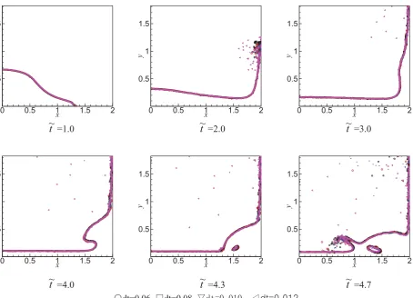
In order to study how the numerical results changes with the different lengths of time steps, the ISPH_R method is employed to simulate the same case as in Fig. 11 by using '~t 0.012, 0.010, 0.008, 0.006 (corresponding to 0.8, 0.67, 0.53 and 0.4 of the CFL (Courant–Friedrichs–Lewy) number calculated by using the velocity equal to ඥʹ݃ܪ) . The free surface profiles at different time instants are depicted in Fig. 12. Generally speaking, the difference between profiles is insignificant, in particular when the time step length is less than 0.01. From the discussions about Figs. 11 and 12, one would see that with use of a time step length of less than 0.01 and more than 3200 particles, the ISPH_R method can yield convergent results in terms of the free surface profiles. It is noted here that compared with Figs. 17 and 18 of Lind et al [21] where no top rigid wall was at y=2, the graphs in Fig. 11 and 12 show slight more isolated particles. This may be attributed partially to the reflection by the top rigid wall after impact. In addition, the results may also be improved by adopting an adaptive time-step technique and by combining the new technique for solving the pressure Poisson equation with other particle stabilising (e.g., particle shifting) techniques and with other free surface identification methods, other than these employed in this paper.

L

t ~

=1.0 ~t =2.0 t~=3.0

t ~

=4.0 ~t =4.3 ~t =4.7 ƻ M=800 ƶ M=1250 Ƹ M=1800 ͪ M=3200 ሩM=5000 ሧ M=7200

Fig. 11 Free surface profile comparison corresponding to different particle numbers by using the ISPH_R method

The convergence property is now examined in terms of the pressure, which is more critical. The time histories of pressure at Point p₂ on the right vertical wall with the height of h₂ 0.05Hare presented in Fig.13(a) for the cases with the different particle numbers. The average error is calculated by

¦

¦

i i N

i

i i

p p p p

Er

1 2 0 , 1

2 0 , )

( , where p_i,0is the pressure for M 7200 _{at different time step} i, which is plotted in Fig. 13(b). The results of Fig. 13 confirm that with the particle number increasing, the results of pressure seem to be convergent. Other methods (traditional SPH, ISPH and CISPH2) are also applied to simulate this case. The results of pressure at Point p₂ from them for M 7200 are compared in Fig. 14. It can be seen that the spurious oscillations in the pressure time histories produced by traditional SPH is very large, the fluctuations of pressure obtained by ISPH and CISPH2 methods much smaller but still visible while the time history from the ISPH_R method is much smoother. In addition, Table 1 compares the CPU times used by different methods to yield the results in Fig. 14. It can be seen that the ISPH_R method does not only provide smoother pressure time history but also spend much less CPU time, which is 86.7% of that used by the ISPH, 80% of that by CISPH2 and 40.2% of that used by the traditional SPH method for this case.

x

y

0 0.5 1 1.5 2 0.5

1 1.5

x

y

0 0.5 1 1.5 2 0.5

1 1.5

x

y

0 0.5 1 1.5 2 0.5

1 1.5

x

y

0 0.5 1 1.5 2 0.5

1 1.5

x

y

0 0.5 1 1.5 2 0.5

1 1.5

x

y

0 0.5 1 1.5 2 0.5

t~=1.0 ~t =2.0 t~=3.0

t~=4.0 ~t =4.3 t~=4.7

ƻdt=0.06ƶdt=0.08ͪGW ͑ ሧΕΥͮͣ͑͟͢͡͡

Fig. 12 Free surface profile comparison corresponding to different time step lengths by using the ISPH_R method (M 3200)

0. 0 0. 5 1. 0 1. 5 2. 0 2. 5 3. 0 3. 5 4. 0 - 0. 5

0. 0 0. 5 1. 0 1. 5 2. 0 2. 5

p/

U

gH

t ( g/ H)1/ 2

M=800 M=1800 M=3200 M=5000 M=7200

2. 8 3. 0 3. 2 3. 4 3. 6 3. 8 - 1. 8

- 1. 6 - 1. 4 - 1. 2 - 1. 0 - 0. 8 - 0. 6

Lo

g

(

E

rp

)

L og( M)

(a) (b)

Fig. 13 Convergence test of pressure whenh₂ 0.05H (a) the pressure time histories; (b) the errors, corresponding to different number of particles

x

y

0 0.5 1 1.5 2 0.5

1 1.5

x

y

0 0.5 1 1.5 2 0.5

1 1.5

x

y

0 0.5 1 1.5 2 0.5

1 1.5

x

y

0 0.5 1 1.5 2 0.5

1 1.5

x

y

0 0.5 1 1.5 2 0.5

1 1.5

x

y

0 0.5 1 1.5 2 0.5

1. 0 1. 2 1. 4 1. 6 1. 8 2. 0 2. 2 2. 4 2. 6 2. 8 3. 0 - 2. 0

- 1. 5 - 1. 0 - 0. 5 0. 0 0. 5 1. 0 1. 5 2. 0 2. 5 3. 0 3. 5 4. 0 4. 5 5. 0 5. 5 6. 0

1. 4 1. 5 1. 6 1. 7 1. 8 1. 9 2. 0 0. 5

1. 0 1. 5 2. 0 2. 5 3. 0

p/

U

gH

t ( g/ H)1/ 2

SPH I SPH CI SPH2 I SPH_R

p/

U

gH

t ( g/ H)1/ 2

SPH I SPH CI SPH2 I SPH_R

Fig. 14 Comparison of breaking wave impact obtained by different methods

Table 1. CPU time comparison of different methods for dam breaking wave simulation

Scheme Time step (t g/H )

Stepping number

CPU time(s)

SPH 0.000313 12771 4086

ISPH 0.002 2000 1893

CISPH2 0.002 2000 2046

ISPH_R 0.008 500 1641

In order to make further comparison between the results from the methods, another benchmark case for dam breaking flow is considered. In this case, L 2.0m, H 0.5L, D 5.3667H. For this case, the pressure time histories at p₂ obtained by the CISPH2 and ISPH_R methods with M 7200 is compared with the experimental data [36] in Fig. 15. This shows that the pressure time history from the ISPH_R method is smoother, though both have similar agreement with the experimental data.

2. 0 2. 5 3. 0 3. 5 4. 0 4. 5 5. 0 5. 5 6. 0 6. 5 7. 0 7. 5 8. 0 8. 5

- 0. 4 0. 0 0. 4 0. 8 1. 2 1. 6 2. 0 2. 4

p/

U

gH

t ( g/ H)1/ 2

Ex p[ 36] CI SPH2

2. 0 2. 5 3. 0 3. 5 4. 0 4. 5 5. 0 5. 5 6. 0 6. 5 7. 0 7. 5 8. 0 8. 5 - 0. 4

0. 0 0. 4 0. 8 1. 2 1. 6 2. 0 2. 4

p/

U

gH

t ( g/ H)1/ 2 Ex p[ 36]

I SPH_R

(b)

Fig. 15 Comparison of pressure time histories at p₂with experimental results [36] and different SPH methods

3.2. Sloshing waves in a moving tank

In order to further show the properties of the ISPH_R method, this section gives the results of sloshing waves in a moving tank. The cases for small amplitude sloshing and violent sloshing will be considered to compare the numerical results with analytical solution [37], and with experimental data [38], respectively.

The geometry of the sloshing tank is illustrated in Fig.16. The tank length is Lˈits height h, and the water depth is d. There is a pressure sensor mounted on the left wall. The height between the sensor and bottom is h₁. The sway displacement of the tank is given byXs a₀(1cos:t), where a0 and : are the

amplitude and the frequency of the motion, respectively. In the simulation, the moving coordinate system fixed to the tank is employed to simplify the implementation of solid boundary conditions as in [42].

3.2.1. Small amplitude sloshing

h1

h

d

l p1

Fig. 16 Sketch of sloshing tank

There are two reasons to simulate this case. One is that when the motion amplitude, i.e. a₀:/ gd , of the tank is small, and the frequency is not close to the natural frequency of sloshing waves in the tank, the free surface elevation can be analytically expressed by

¦

f

1

) 2 ( cos ) ( 1

n

n

n d

L x k t B g

K (34)

1 (₂ 1) 2 ₀ cos _{2 2} cos :

: : :

n

n n

n n n

n n

t t

U L

k B

Z Z Z

Z Z

(35)

where k_n nS /LˈZ_n gk_ntanhk_nd . More details about the solution can be found in [37]. The second reason for considering this case is that the error of numerical methods can be precisely estimated and so their behaviours can be systematically investigated. For this purpose, d 0.5m, L 2d ,a₀ 0.001dare selected and different numbers (M) of particles are used, that is 288, 450, 800, 1250, 1800, 3200, 5000 and 7200 with the corresponding non-dimensional particle sizes being s 0.0417, 0.033, 0.025, 0.02, 0.0167, 0.0125, 0.01, 0.083, respectively. Fig. 17 gives the comparison of free surface elevations on the left tank wall, which are calculated by the analytical solution in Eq. (34) and by the ISPH_R method for :/Z₁ 0.8 (only the results corresponding to 288, 800, 3200 and 7200 are plotted for clarity). This figure indicates that the results of the ISPH_R method for this case become very close to the analytical solution when the number of particles is 800 or more. The results of the ISPH_R method are also compared with those from the SPH, ISPH and CISPH2 in Fig. 18, which are also produced by using 800 particles but different time step length. Non-dimensional time stepping length ('~t ) is 0.008 for the ISPH_R, 0.002 for ISPH and CISPH2, and 0.000313 for SPH. From Fig. 18, it can be seen that the results of the SPH has a good agreement with analytical solution at first three periods, but with the simulation going longer, numerical dissipation in the wave amplitude become evident. In addition, in the time range (such as 35 to 40) of short and small waves, the traditional SPH method cannot catch the detail correctly. In contrast, the results from the ISPH, CISPH2 and ISPH_R method do not exhibit such dissipation and can well catch the details of short and small waves. In order to quantitatively show the behaviours of the methods, Fig. 19 presents the errors of numerical results relative to the analytical solution corresponding to different numbers of particles employed. In this

figure, the error is computed by using

¦

¦

t

t N

i a i N

i

a i i

Er

1 2

, 1

2

, K

K K

K , where Ki,ais the wave elevation

on the left wall of analytical solution at i-th time step, K_iis the numerical result at the time instant, N_t is total time steps in the simulation duration of ~t 50.0. Fig. 19 clearly shows that the error of results from the ISPH_R method is considerably smaller than those of SPH, ISPH and CISPH2 methods. It is a little surprising that the two curves for ISPH and CISPH2 methods are very close to each other in this case. In other words, to achieve any specified accuracy, the ISPH_R method needs much less number of particles (or larger particle sizes) than others. For example, corresponding to Log(Er_K) 3.4, the particle size required by ISPH_R, CISPH2, ISPH and SPH methods are Log(s)|-1.62, -1.85, -1.86 and -1.96, respectively. In order to explore the properties of the methods in another way, Fig. 20 depicts the CPU time spent by all the methods corresponding to different numerical errors on the same computer. One can see from Fig. 20 that the ISPH_R method needs much less CPU time to achieve the same level of accuracy. For example, corresponding to Log(Er_K) 3.35, the CPU times spent by the ISPH_R, CISPH2, ISPH and traditional SPH methods are Log(CPU_t)| 2.76, 3.24, 3.19, and 3.70, which are CPU_t575, 1737, 1548 and 5011 seconds, respectively.

0 20 40

0. 496 0. 500 0. 504

(

K

+d

)

/

L

t ( g/ L )1/ 2

Anal y t i c al r es ul t s M=288

M=800 M=3200 M=7200