The Active Young Solar-Type Star HR 1817
(= HD 35850)
A dissertation submitted by
Matthew Wayne Mengel
B.IT, Grad.Dip.IT
For the Award of
Master of Philosophy
Department of Biological and Physical Sciences
University of Southern Queensland
© Copyright
Abstract
The active F dwarf HR 1817 represents the upper temperature extreme of what are broadly termed solar-type stars – stars which have the same internal structure as the Sun, albeit in this case with a much smaller convective zone. To date, studies of the active surface features and magnetic fields of solar-type stars have been restricted to G and K dwarfs. This thesis investigates the surface and magnetic features of HR 1817 using the techniques of Doppler and Zeeman Doppler Imaging, resulting in tomographic maps of the stellar surface and magnetic field.
Cooler stars than HR 1817 exhibit large polar spots, and while HR 1817 also exhibits a polar spot, it is not nearly as large as those usually seen. The lower-latitude surface features of HR 1817 are weak but well defined and cover a relatively small area of the stellar surface. Total spot coverage is relatively small (~ 1.7 - 2%).
Zeeman Doppler Imaging reveals that HR 1817 exhibits a richly-detailed, though weak magnetic topography. A ring of azimuthal field appears around the pole, while the radial field exhibits many well-defined and distinct bipolar mid-latitude magnetic features, perhaps indicating a more dominant interface dynamo as opposed to the posited distributed dynamo of cooler active dwarfs.
Certification of Dissertation
I certify that this dissertation contains no material accepted for the award of any other degree or diploma in any university. To the best of my knowledge, it contains no material published or written by another person, except where due reference is made in the text.
Signature of Candidate Date
ENDORSEMENT
Acknowledgements
The road to completing this thesis has been long and difficult for me, especially while working a demanding job more than full-time in the University’s IT Department. I would like to thank my principal supervisor Brad Carter for staying the course with me and being so supportive and understanding when work and illness have meant that I couldn’t give this thesis the attention it needed and deserved.
Enormous thanks also to my associate supervisor Stephen Marsden for all his assistance and advice. The quality of the analysis and output has been immeasurably improved by his input.
I would like to also thank Jean-François Donati for his assistance, and for allowing me the use of the ESpRIT code. Thanks as well for Meir Semel for the use of the polarimeter at the AAT. Pascal Petit also provided assistance in getting some of the prettier maps out using my ancient code base.
This work could not have been possible without the excellent work by all at the AAT, including the operators, duty astronomers, technical staff and administrative staff.
Thanks go to Ruth Hilton and all in the USQ Research and Higher Degrees office. I have tested their patience in getting this all done, but they have stuck by me and given me assistance without which it would have been so easy to give up. Also, to my supervisors and colleagues in the Information Technology Services department at USQ, thanks for doing what you could when I needed to get away to observe, or to get this thing written.
Contents
Abstract... iii
Certification of Dissertation... iv
Acknowledgements ... v
List of Figures... ix
List of Tables ... xii
1 Introduction... 1
1.1 The Sun ... 2
1.1.1 Solar Magnetic Activity... 2
Sunspots ... 2
1.1.2 The Solar Interior... 4
1.2 The Solar Dynamo ... 7
1.2.1 The Babcock Model... 7
Stage 1: The Ω Effect... 7
Stage 2: Surface Eruption and the α Effect... 8
Stage 3: Opposite Polarity ... 9
1.2.2 A Refined Model... 9
1.3 Solar-Type Stars... 11
1.3.1 Stellar Dynamos... 11
1.4 Stellar Magnetic Activity... 13
1.4.1 Starspots... 13
Doppler Imaging ... 13
1.4.2 Stellar Surface Magnetic Field... 16
1.4.3 Differential Rotation ... 20
1.5 The Active Young F Dwarf HR 1817 (= HD 35850) ... 22
1.5.1 Physical Parameters of HR 1817 ... 22
1.6 Summary... 24
2 Instrumental Setup, Observations and Analysis... 26
2.1 ZDI at the Anglo-Australian Telescope... 26
Instrumental Considerations ... 26
Semel Polarimeter... 27
2.1.1 Instrumental Setup ... 29
Initial Detection: 9 December 2000... 29
Doppler and Zeeman Doppler Imaging: 23 December 2001 - 2 January 2002 .... 30
2.2 Observations ... 31
Initial Detection: 9 December 2000... 31
Doppler and Zeeman Doppler Imaging: 23 December 2001 - 2 January 2002 .... 32
2.3 Analysis: Spectral Extraction... 37
Why use ESpRIT?... 38
Frame Calibration (Geometric)... 38
Frame Calibration (Wavelength) ... 39
Extraction of Intensity Spectra... 39
Extraction of Polarized Spectra ... 40
2.4 Analysis: Least Squares Deconvolution ... 42
Magnetic Detection... 44
2.5 Analysis: Maximum Entropy Image Reconstruction... 44
3 Results and Discussion... 47
3.1 Results: Magnetic Field Detection on HR 1817 ... 47
Initial Estimate of Radial Velocity ... 49
3.2 Results: Doppler Imaging of HR 1817 ... 50
December 23, 2001 ... 50
December 26, 2001 ... 51
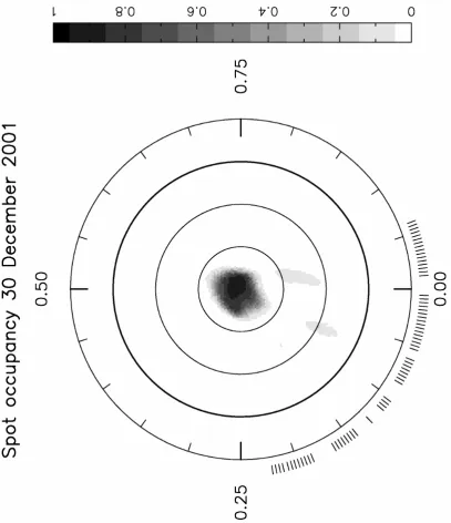
December 30, 2001 ... 51
Combined Image... 61
3.3 Results: Zeeman Doppler Imaging of HR 1817 ... 66
3.4 Results: Differential Rotation of HR 1817 ... 72
3.5 Results: Measurement of Stellar Inclination and Radial Velocity... 74
3.6 Discussion: HR 1817 ... 75
Spot Coverage... 76
Magnetic Topology... 78
Differential Rotation ... 80
3.7 In Conclusion ... 82
Appendix A ... 88
Differential Rotation of HR 1817 using Spots... 88
Appendix B ... 89
List of Figures
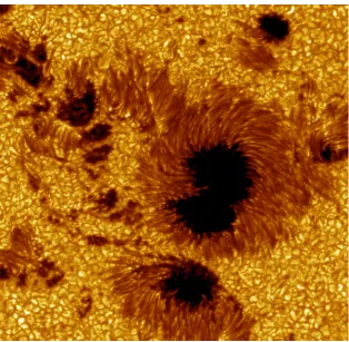
1.1 A Complex Sunspot Group... 3
1.2 Solar Butterfly and Sunspot Coverage Diagram (1874 - 2004)... 4
1.3 The Solar Interior... 6
1.4 Measurement of differential rotation through the solar convective zone (SOHO Data) ... 6
1.5 The solar magnetic cycle ... 8
1.6 Joy's Law... 9
1.7 Principles of Doppler Imaging... 15
1.8 Principles of Zeeman Doppler Imaging... 18
1.9 HR 1817... 23
2.1 Polarimeter setup for CFHT... 28
3.1 Detection of Magnetic Field on HR 1817 December 9, 2000 ... 48
3.2 Maximum entropy fits to LSD Stokes I profiles, 23 December,2001 ... 53
3.3 Maximum entropy brightness image of HR1817, 23 December, 2001 ... 54
3.4 Maximum entropy fits to LSD Stokes I profiles, December 26, 2001 ... 55
3.5 Maximum entropy brightness image of HR 1817, 26 December 2001 ... 56
3.7 Maximum entropy brightness map of HR1817, 30 December, 2001 ... 58
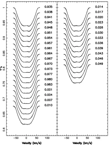
3.8 Maximum entropy fits to LSD Stokes I, 2 January 2002 ... 59
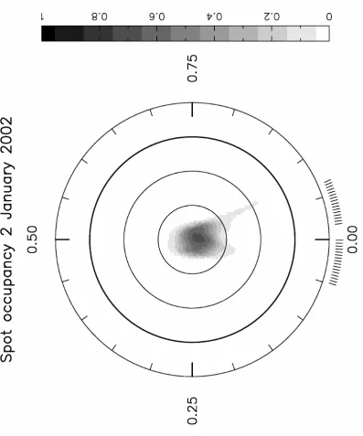
3.9 Maximum entropy brightness map of HR1817, 2 January 2002 ... 60
3.10a Maximum entropy fits to LSD Stokes I, all nights December 2001 - January 2002 ... 62
3.10b Maximum entropy fits to LSD Stokes I profiles, all nights December 2001 - January 2002 ... 63
3.11 Maximum entropy brightness map of HR 1817, all nights combined December 2001 - January 2002... 64
3.12 Maximum entropy brightness map of HR 1817, all nights December 2001 - January 2002, spherical projection ... 65
3.13 Maximum entropy fit to Stokes V profiles, all nights December 2001 - January 2002 ... 69
3.14 Maximum entropy magnetic maps of HR 1817, all nights December 2001 - January 2002 ... 70
3.15 Maximum entropy magnetic maps of HR 1817, all nights December 2001 - January 2002... 71
3.16 Surface differential rotation χ2 minimization for HR 1817 ... 73
3.17 Surface differential rotation χ2 minimization for HR 1817 ... 73
3.18 χ2 minimization for stellar inclination angle... 74
3.19 χ2 minimization for radial velocity ... 75
3.22 ∆Ω versus Teff... 81
A.1 Surface differential rotation χ2 minimization for HR 1817 using spots... 88
B.1 Fractional spottedness of AB Dor... 89
B.2 Fractional spottedness of HR 1099 ... 89
B.3 Fractional spottedness of LQ Hya... 90
List of Tables
1.1 List of stars with measured differential rotation ... 21
1.2 Parameters of HR 1817... 23
2.1 Log of Observations of HR 1817, 9 December 2000 ... 31
2.2 Log of Observations of HR 1817, 23 December 2001 - 2 January 2002... 33
3.1 Polarization cycles for 9 December 2000 ... 48
Chapter 1
Introduction
The Earth’s nearest stellar neighbour in space is the Sun. A typical G2 dwarf star,
the Sun is the only dwarf star whose surface can be resolved directly. Hence the Sun is
an archetype for studies with much to tell us about similar stars. However, this
solar-stellar connection is a reciprocal arrangement in that the study of other dwarf stars can
also give us insights into the activity of the Sun. Observations of G and K dwarfs using
different techniques have shown that the Sun is not alone in exhibiting phenomena
indicating an active atmosphere such as spots and flares (Schrijver and Zwann, 2000).
While the Sun has been extensively studied, these studies have been over a very
short period; a tiny fraction of the Sun’s life. This means that all we have is a mere
snapshot of the Sun as it is now. This is useful in itself, however the study of different
stars at differing ages, masses, temperatures and levels of activity allows us to not only
be able to infer the evolution of the Sun and in particular its early history (Baliunas,
1991).
1.1 The Sun
The Sun is a main-sequence G2V dwarf star which is approximately 4.5 x 10⁹ years old.
Due to the proximity of the Sun, it is the star about which we have the greatest amount of
observational data. These data provide the opportunity to test the theories of stellar
interiors and atmospheres.
1.1.1
Solar Magnetic Activity
Magnetic fields are responsible for almost all active phenomena we see on the Sun.
Sunspots, prominences and flares are but a few of the most obvious phenomena. Of
these, the best-known manifestations of solar magnetic activity are sunspots.
Sunspots
Sunspots are dark parts of the Sun’s surface which are significantly cooler than the
surrounding area. Sunspots range in size up to ~ 30 x 106 m and usually develop and
decay over periods of a few days to weeks. Sunspots are significantly cooler (~ 4000 K)
Figure 1.1 A complex sunspot group taken 15 July 2002 by the 1 metre Swedish Solar Telescope
on La Palma. This shows the darkening of the sunspot area compared with the surrounding photosphere. (Obtained from web site http://www.solarphysics.kva.se/; Royal Swedish Academy of Sciences)
Sunspots occur where the solar magnetic field breaks through the surface. The presence
of the intense magnetic field retards the normal convective process in the photosphere.
Sunspots are generally found in groups (see Figure 1.1), and typically a dominant sunspot
leads the group in the direction of solar rotation and one or more sunspots follow.
Despite the complexity of sunspot groups and the attendant magnetic fields in the region
of a sunspot group, the field is essentially bipolar with the trailing spots having the
opposite polarity to the leading spot.
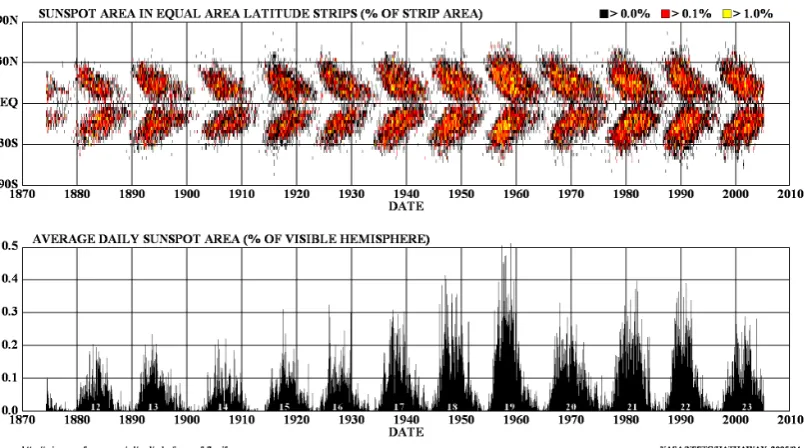
The number of sunspots visible on the solar surface varies according to an 11-year
[image:15.595.141.456.102.409.2]fact, the cycle lasts 22-years: each 11-year cycle is followed by a reversal in the direction
of the Sun’s magnetic field.
While an individual sunspot remains at a constant latitude, during the solar cycle,
the latitudes of new sunspots slowly migrate towards the equator (Figure 1.2, upper
panel). However, they usually appear in a band no further than 40° and no closer than 5°
either side of the equator. The migration of sunspots results in the famous “butterfly
diagram”.
Figure 1.2 Solar butterfly (upper) and sunspot coverage (lower) diagrams from 1874 until 2004.
The butterfly diagram (above) shows how the sunspot locations migrate towards the equator during the 11-year solar cycle. The lower diagram shows how the coverage of the solar disc changes over the same cyclical period. Diagram from D.H. Hathaway, NASA Marshall Flight Center. (Obtained from http://science.nasa.gov/ssl/pad/solar/images/bfly.gif)
1.1.2
The Solar Interior
The interior of the Sun consists of 3 layers: the core, the radiative zone and the
[image:16.595.92.495.330.554.2]The core is where thermonuclear reactions take place to convert hydrogen into
helium via the proton-proton chain. The core occupies around one quarter of the solar
radius, but contains ~ 50% of the solar mass. The boundary between the core and the
radiative zone is defined as where the density and temperature fall below that required for
nuclear reactions to occur.
In the radiative zone energy from the core is absorbed and re-emitted in random
directions. This so-called “random walk” process from the core to the convective zone
can take up to one million years. It is believed that the radiative zone rotates almost as a
solid body, and recent observations by the SOHO spacecraft confirm this (see Figure
1.4). The radiative zone extends from the core to approximately 75% of the stellar
radius.
Finally, the convective zone is the outermost layer of the solar interior. At the
base of the convective zone, the temperature is only around 2 x 10⁶ K. At this point,
some of the heavier ions such as iron, calcium and nitrogen can retain some of their
electrons, which makes the stellar material more opaque to radiation. This traps heat
which makes the fluid unstable and it starts to convect. The convective actions carry heat
to the stellar surface quite rapidly. The stellar material cools and expands as it rises,
resulting in the surface temperature of ~ 5780 K.
The upper layer of the Sun is fluid in nature, and so the equator rotates at a
different rate than the poles (differential rotation). This has been known since Galileo
first started tracking sunspots. Measurements from the SOHO spacecraft indicate that
this rotation is maintained through the convective zone (see Figure 1.4). However, at the
convective zone disappear. This change in fluid flow characteristics results in
rotationally generated shears. This interface layer plays a key part in the generation of
the solar magnetic field.
Figure 1.3 The solar interior. The temperature and density of the stellar material falls rapidly as
distance from the stellar core increases. (Taken from web site: http://cse.ssl.berkeley.edu/segwayed/lessons/sunspots/research2.html)
Figure 1.4 Measurements from the SOHO spacecraft show that differential rotation is
[image:18.595.204.391.186.376.2]1.2
The Solar Dynamo
The solar magnetic field is thought to be generated by the motions of fluid plasma in the
interface layer between the radiative and convective zones, known as the tachocline.
Kinetic energy is transformed into magnetic energy via a magnetohydrodynamic process
and this flux eventually emerges at the solar surface.
1.2.1 The Babcock Model
Babcock (1961) posited that the mechanisms which comprise the Sun’s magnetic cycle
and therefore the dynamo which is responsible are threefold. The process described
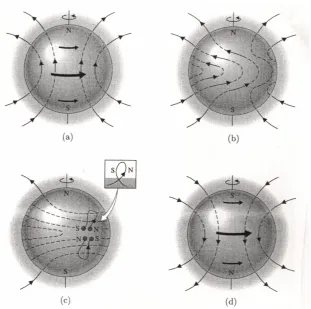
below is illustrated in Figure 1.5.
Stage 1: The Ω Effect
Initially, the overall solar magnetic field is approximated by a poloidal dipole field
symmetric about the Sun’s rotational axis. This original poloidal field is transformed into
a toroidal field (where the magnetic field lines are wrapped around the Sun) due to
Figure 1.5 The Solar Cycle. The initial poloidal field (a) is twisted into a toroidal field (b) by
differential rotation (the Ω effect). Turbulent convection twists the field lines into magnetic ropes
(c, the α effect). As the cycle progresses, successive sunspot groups migrate toward the equator
where magnetic field reconnection reestablishes the poloidal field, with reversed polarity (d). (Carroll and Ostlie, 1996)
Stage 2: Surface Eruption and the α Effect
Turbulent convection then twists the magnetic field lines into magnetic ropes – regions of
intense magnetic fields. This is known as the α effect. The buoyancy produced by
magnetic pressure causes the magnetic ropes to rise to the surface. At this point, bipolar
active regions are formed as the toroidal flux tubes erupt through the solar surface.
The α effect results in sunspot groups that obey Joy’s law – the leading spot of a
bipolar pair is located at a lower latitude than the trailing spot. Thus the following spot
[image:20.595.143.455.102.411.2]Figure 1.6 Joy’s Law. The leading spot of a bipolar pair is located at a lower latitude than the
following spot. (From website http://science.msfc.nasa.gov/ssl/pad/solar/images/joys_law.jpg)
In combination, these effects act to neutralize and reverse the global poloidal
field.
Stage 3: Opposite Polarity
Finally, the process is repeated with a reversed polarity. Stages 1 and 2 take
approximately 11 years. The repetition with the reversed polarity results in the full
22-year solar cycle.
1.2.2
A Refined Model
While the Babcock model illustrates the major parts of the magnetic cycle, it is not
complete and is a simplified view. For example, the Babcock model of the Sun's dynamo
assumed that the twisting is produced by the effects of the Sun's rotation on very large
convective flows that carry heat to the Sun's surface. However, this assumption resulted
in amounts of twisting that were far too much and produced magnetic cycles that are only
Schrijver and Zwaan (2000) present a more refined model than Babcock. Density
stratification in the convective zone makes solar convection highly anisotropic. Upflows
are weak and broad, while downflows are characterized be a complex, evolving network
of lanes and plumes. These downflow plumes are turbulent and they possess substantial
rotational components which may amplify fields through the α effect. These fields are
then moved downward by the anisotropic convection and accumulate in the overshoot
region. Plumes may pull some of this flux upwards and return it to the convection zone
where further amplification may take place before being pumped down again.
Differential rotation in the tachocline (the Ω effect) creates strong, coherent toroidal flux
tubes by stretching and amplifying the disorganized field. As the field becomes stronger,
it rises toward the surface in blobs. The Coriolis force acting on these blobs twists them
in a systematic way which depends on latitude (the α effect). Weaker structures can be
destroyed by turbulent convection, but stronger fields remain coherent and emerge from
the surface as bipolar active regions.
Where an active region is close to the pole, the following (i.e. higher latitude)
polarities reconnect with the magnetic field at the pole, while leading polarities tend to
connect with other active regions. Eventually, the active regions nearest the equator in
opposite hemispheres reconnect. These reconnected loops now have a poloidal
component which is in the correct direction for the next part of the magnetic cycle. The
flux then retracts into the convective zone and the interface layer receives a reversed
1.3
Solar-Type Stars
While there is an understanding of the solar dynamo, this understanding is broad and
many of the details are unknown. For example, the mechanisms of flux retraction are as
yet unknown and unobserved. Studying stars other than the Sun allows the expansion of
knowledge about dynamos in general and the refinement of the understanding of the solar
dynamo in particular.
The Sun is a main-sequence G2 dwarf, and as has been noted previously, the Sun
has a radiative and a convective zone. We can broadly define stars with the same interior
structure as the Sun as “solar-type” stars. Stars which have a mass greater than
approximately 1.3 solar masses lack a convective zone, while stars of mass lower than
approximately 0.3 solar masses should be entirely convective. This encompasses stars
from mid-F to early-M spectral types.
1.3.1
Stellar Dynamos
Given that solar-type stars have similar internal structure as the Sun, these stars should
exhibit dynamo processes and hence magnetic phenomena in their atmospheres. In fact it
has been shown that this is the case (Cram and Kuhi, 1989).
However, while in the solar dynamo it is assumed that the regeneration of the
poloidal field is as a result of the α effect, it is theoretically possible for the regeneration
to be as a result of the α effect or the Ω effect (i.e. differential rotation). This gives rise to
• αΩ: This is the type of dynamo exhibited by the Sun. In this type of dynamo,
periodic behaviour is observed, and the field structures generated are asymmetric.
The α term is much smaller than the Ω in the conversion of the poloidal field into
a toroidal structure.
• α2: The type of dynamo exhibited by the Earth. This dynamo generates
symmetrical field structures. The Ω component is much smaller than the α, which
becomes dominant in the poloidal regeneration and toroidal construction.
• α2Ω: In this dynamo, the α and Ω terms are of similar magnitude in the
generation of the toroidal field.
While present theory indicates that the solar dynamo is generated in the interface
layer between the radiative and convective zones, Donati et al. (1992; 1999; 2003a) ,
Donati and Cameron (1997) and Donati (1999) have indicated that active solar-type
stars may exhibit what has been termed a distributed dynamo – where the dynamo
process is distributed throughout the convective zone of the star.
While this means that the study of stellar magnetic fields may not be directly
applicable to solar study, it is valuable in describing the continuum of dynamo
processes, and in fact may be valuable in describing historical aspects of the Sun’s
magnetic field; especially when the Sun was young and rotating much faster than
presently. Magnetism is undeniably a strong influence on the behaviour of the Sun,
and so it may be on solar-type stars irrespective of the dynamo mechanism they
1.4
Stellar Magnetic Activity
Given that solar-type stars have a similar internal structure to the Sun, and given that
magnetic phenomena are visible on the Sun, it is reasonable to assume that similar
magnetic phenomena should be present on solar-type stars. In fact this is the case, with
observations of different types showing the presence of magnetic activity similar to that
of the Sun.
1.4.1
Starspots
Starspots, like sunspots are darker areas which are cooler than the surrounding stellar
surface due to magnetic activity. As a star rotates, starspots moving across the visible
hemisphere of the star result in small variations in brightness (of the order of
0.1 magnitude or less).
Doppler Imaging
Even the nearest dwarf stars to the solar system are so distant that even the largest
telescopes cannot resolve their surfaces. Doppler Imaging (also known as DI) is a
spectroscopic method which can be used to determine the distribution of starspots across
the stellar surface.
Vogt and Penrod (1983) coined the term Doppler Imaging in relation to stellar
surface imaging and since this seminal paper, many stars (over 50) have been
investigated using the technique.
On a rapidly-rotating star, the individual spectral lines are broadened by the
“bump” in the observed spectral line profile (Figure 1.7; right panel). In addition,
because the light is “missing” from the dark spot, a slight reduction in the overall
intensity of the spectral line is observed. As the star rotates, carrying the dark spot across
the stellar disc, the bump in the line profile changes its Doppler shifted position relative
to the stellar rotation axis – the bump moves across the line profile.
By observing the star over a series of rotational phases, a map of the locations of
starspots on the stellar surface may be created. The principles of Doppler Imaging are
described in depth in Vogt et al. (1987), Rice et al.(1989) and Hussain, (1999).
In order to obtain sufficient resolution in longitude, Doppler Imaging is only
effective when the stellar target rotates relatively rapidly (v sin it 20 kms-1 – cf. solar
v sin i≈ 2 kms-1). With very few exceptions (such as EK Dra; Strassmeier and Rice
(1998)) most of the stars to date investigated using Doppler Imaging have v sin i greater
than 20 kms-1 with some ranging up to ~ 130 kms-1 (“Speedy Mic”; Barnes et al. (2000))
and beyond (VXR45A rotates at ~ 248 kms-1 (Marsden et al. (2004)).
To date, for solar-type stars, the technique of Doppler Imaging has been
exclusively applied to G and K dwarfs (see Strassmeier, 2001). Almost always, these
objects observed have exhibited polar spots in addition to many low- and high-latitude
features. This is in contrast to the Sun where sunspots exclusively inhabit bands ~ ± 30°
Figure 1.7 The spectral line of a rapidly rotating star is broadened by the Doppler effect (left
panel – full stellar disc). The presence of a dark spot (A) in the right panel results in (1) a continuum effect due to the missing light from the spot and (2) a bump in the profile which is Doppler shifted by an amount corresponding to its distance from the stellar rotation axis. (From slides from review talk given at the International Workshop on Astro-tomography, Brussels by Andrew Collier-Cameron (July 2000). Obtained from http://star-www.st-and.ac.uk/~acc4/coolpages/dopreview/sld003.htm).
Schüssler et al. (1996) and Granzer et al. (2000) have done theoretical work on
the emergence of flux tubes and the resulting location of star spots. They show that only
the very youngest stars which exhibit deep convective zones should have polar spots.
Zero-age main sequence objects should show spots which appear at higher latitudes as
rotational rates increase, but never exhibit true polar spots. These theoretical studies gave
rise to debates about whether polar spots were real or simply artifacts of the techniques
used to construct maps. Papers on the subject include Byrne, 1996; Unruh and Cameron,
1997. Flux emergence models such as those in Granzler et al (2000) cannot explain the
observation of polar spots on main sequence stars, however polar spots can be explained
if magnetic flux tubes undergo a migration towards the pole. It now seems generally
accepted that the phenomenon of polar spots is actual rather than artifactual. A new
study of the eclipsing binary SV Cam (Jeffers et al., 2005) has also shown direct evidence
In addition to polar spots, Donati et al. (2003a) show that for rapidly-rotating
solar-type stars, spot coverage can be up to ~ 10% of the visible stellar surface. This is a
conservative measurement, given that the mapping techniques minimize the spot area
required to fit the observed profiles. In any case, this proportion of spot coverage is over
ten times that observed on the solar surface.
The presence of polar spots and the large spot coverage would tend to indicate
that either the dynamo processes in these rapidly-rotating solar-type stars are much
stronger than those in the Sun, or that the dynamo processes are fundamentally different
to the solar dynamo, or both.
1.4.2
Stellar Surface Magnetic Field
In the presence of a magnetic field, spectral lines are seen to split. This is known as the
Zeeman effect. While star- and sunspots are manifestations of surface magnetic fields,
the Zeeman effect has the potential to allow the direct investigation of the magnetic fields
themselves.
When encountering a magnetic field parallel to the line-of-sight, light from the
source is split into three components: two symmetric oppositely circularly polarized
σ-components and a central linearly-polarized π-component. When the magnetic field is
perpendicular to the line-of-sight, the σ-components are linearly polarized perpendicular
to the magnetic field and the π-component linearly polarized parallel to the magnetic
field. The polarization parameters are often expressed in terms of the Stokes parameters,
where parameter I is a measure of the total power in the wave, Q and U represent the
While some work has been done in measuring the magnetic field directly based
on the Zeeman effect on certain sensitive lines in stellar spectra (Saar, 1988), the effect is
small, and also results in only the average field over the entire visible stellar surface.
Hence, these methods do not reveal any information about the magnetic field topology.
Zeeman Doppler Imaging
Zeeman Doppler Imaging (also known as ZDI) is a technique which is used to detect
stellar magnetic fields and also resolve the geometry of the magnetic field across the
stellar surface. Other methods which integrate the field over the stellar surface cannot do
this as features of opposite polarity cancel each other out. Utilizing high resolution
echelle spectropolarimeters, stellar magnetic fields can be detected through the Zeeman
signatures they generate in the shape and polarization state of spectral line profiles.
Initially suggested by Semel (1989), the technique utilizes the same mechanisms as
Doppler Imaging (DI) to provide longitudinal resolution, combined with the polarization
information which gives information about the orientation of the magnetic field. Donati
et al. (2003a) illustrate the ability to map the three components of the magnetic field
(azimuthal, meridional and radial).
Like conventional DI, ZDI is best applied to rapidly-rotating stars because the
signatures of individual unipolar magnetic regions are associated with different Doppler
velocities. This means that bipolar pairs of magnetically active regions no longer
mutually cancel each other out as in methods which average the entire surface of the
Semel (1989), Donati et al. (1989), Brown et al. (1991), Donati and Brown
(1997), and Donati et al. (2003a) all provide details on the ZDI technique. The basic
principles of ZDI are illustrated in Figure 1.8. The visible disc of the star can be divided
into regions of equal rotational velocity. As mentioned in Section 1.4.1, spectral lines are
broadened by the Doppler effect, and the zones of equal rotational velocity contribute to
the spectral lines at a position corresponding to their Doppler wavelength shift. A region
of magnetic activity on the visible disc will result in the polarization of the light emerging
from that area of the star. By observing in left- and right-hand circularly polarized light,
information on the direction and strength of the localized magnetic field can be derived.
Figure 1.8 Principles of Zeeman Doppler Imaging. Two arbitrary magnetic regions of opposite polarity
are present on the stellar disc. The contributions to the stellar spectral line from each of the spots appear at
X1 and X2, separated by Doppler shift in the wavelength domain. The intensity spectrum is I. Each magnetic field induces small opposite wavelengths shifts of the corresponding absorption profile in the right- and left hand circularly polarized spectra (I + V and I – V respectively, where V is the circular
polarization Stoke parameter). The difference between the profiles I + V and I – V results in V, which has a
[image:30.595.174.420.350.622.2]Consider, as shown in Figure 1.8, two arbitrary magnetic regions of opposite
polarity on the stellar disc. The contributions to the stellar spectral line from each of the
spots appear at X1 and X2, separated by Doppler shift in the wavelength domain. The
intensity spectrum is denoted by I(λ). Each magnetic field induces small opposite
wavelength shifts of the corresponding absorption profile in the right- and left hand
circularly polarized spectra (I + V and I – V respectively, where V is the circular
polarization Stokes parameter). The difference between the profiles I + V and I – V
results in V, which has a characteristic shape based on the location of the magnetic
regions on the surface of the star. If the longitudinal resolution provided by the Doppler
effect were not present, then the resulting magnetic signature (V(λ)) would only be an
average for the stellar disc because the opposite-polarity fields would either partly or
completely cancel each other out.
The magnetic signatures are quite small (~0.1% of the continuum level), and so
there are a number of instrumental considerations to maximize the amount of light
captured from the star and to minimize instrumental polarization, and these are discussed
in Chapter 2. In addition, a star must be bright to be able to make it a viable ZDI target.
In most of the examples of ZDI mapping thus far, it appears that the azimuthal
component of the magnetic field is dominant (Donati et al., 2003a). The azimuthal
component of the magnetic field is often evident as rings (Donati et al., 2003a; Donati et
al., 1999; Donati, 1999). As mentioned in the discussion of dynamo types, this has led
postulate that a distributed dynamo is in operation in these stars rather than an
interface-layer dynamo such as that seen in the Sun.
1.4.3
Differential Rotation
It has been long known that the Sun exhibits differential rotation. The Sun rotates every
25 days at the equator and takes progressively longer to rotate at higher latitudes, up to 35
days at the poles. (see Figure 1.4). This means that the equator actually laps the poles
approximately every 120 days. Both Doppler Imaging and Zeeman Doppler Imaging
present a way to measure differential rotation on stars other than the Sun. By observing
either spot features or magnetic features on a stellar surface at different epochs separated
by several days, the rates of rotation at different latitudes can be calculated.
There are three spectroscopic methods by which this can be achieved. One
method is that described by Petit et al. (2002). This method involves the reconstruction
of a single image utilizing a data set covering different epochs, assuming a simplified
solar-type differential rotation law (of the form l eq d l
2
sin )
( =Ω − Ω
Ω ) and using this in
the reconstruction process. Another method involves cross-correlating images from
different epochs, again assuming a solar-type law (Weber et al, 2005). Finally, Cameron
et al. (2002) have developed a new method which tracks the rotational periods of
individual spots on the stellar surface.
The above methods have been used to measure the differential rotation of several
solar type dwarfs (see Table 1.1). All of these stars appear to obey a surface differential
rotation law with the equator rotating faster than the poles. In all cases (except R58 in the
Marsden et. al. 2005 paper), though, the photospheric shear is significantly stronger than
Star Spectral
Type Lap Time (Sun ~ 120d) References
AB Dor K1V ~ 110 Donati and Cameron (1997)
Cameron and Donati (2002) Cameron et al. (2002) Donati et. al. (2003b) LQ Lup G2V-IV 50 ± 10 Donati et al. (2000) PZ Tel K0V-IV 86 ± 14 Barnes et al. (2000)
LQ Hya K0V ~ 80 Kóvári (2002)
Donati et al. (2003b) R58
(=HD 307938) G2V ~ 45 (2004) ~ 250 (2005) Marsden et al. (2004) Marsden et al. (2005)
VXR45A G9V ~ 90 Marsden et al. (2004)
Table 1.1 Listing of stars which have had differential rotation measurements taken
using the methods mentioned.
Interestingly, Donati et al. (2003b) have shown that when the magnetic
features are used for cross-correlation instead of the surface spot features, the rates of
differential rotation are different. This is attributed to the depth in the stellar atmosphere
where the different features are formed and shears within the convective zone. This
means that differential rotation of different features may provide a mechanism to probe
the interiors of solar-type stars.
Also, Donati et al. (2003b) and Cameron and Donati (2002) have observed
changes in the rates of differential rotation in the stars AB Dor and LQ Hya over longer
time periods. For example, the lap time for AB Dor was seen to vary from 71±6 days to
136±18 days. Donati et al. (2003b) speculate that temporal variations in the rates of
differential rotation are due to feedback effects where magnetic energy is converted into
Models of differential rotation developed by Kitchatinov and Rüdiger (1995) and
Rüdiger (1998) show that relative differential rotation Ωdeq Ω
(where dΩ is the difference
in rotation rate between the pole and equator and Ωeq is the rotation rate at the equator)
should decrease in rapid rotators, and should also decrease in stars with larger convective
zones. Barnes et al. (2005) demonstrate that differential rotation appears to increase with
the stellar temperature. However, the number of observations is still small, and a
relationship between differential rotation and various physical stellar parameters is not
clear.
1.5
The Active Young F Dwarf HR 1817
(= HD 35850)
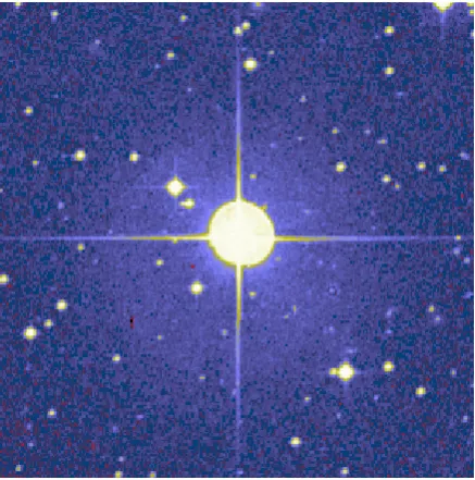
HR 1817 (HD 35850) is a remarkably active young F dwarf star. As an F7V dwarf, it is
at the warm end of the continuum of solar-type stars and its physical parameters
(Table 1.2) such as its rotation rate, level of activity and brightness (Figure 1.9) mean that
it is an ideal target for the techniques of Doppler and Zeeman Doppler Imaging.
1.5.1
Physical Parameters of HR 1817
HR 1817 is of spectral type F7V, is a rapid rotator and has intense X-ray and extreme
ultraviolet (EUV) emission (Tagliaferri et al., 1997). It also exhibits a strong lithium
Parameter Value
Coordinates (2000) 05 27 04.76 -11 54 03.5
Spectral Type F7V
v sin i 50 km s-1
Distance 26.8 pc
B Magnitude 6.8
V Magnitude 6.3
Age ~ 12 Myr
Radius 1.18 R
Mass 1.15 M
[image:35.595.189.408.347.568.2]
Table 1.2 Parameters of HR 1817. From Tagliaferri et al. (1997); Gagné et
al. (1999); Mathioudakis and Mullan (1999); Zuckerman et al. (2001). Note that none of the original sources quote errors for these values.
Figure 1.9 HR 1817. Image from NASA SkyView
As Gagné et al. (1999) show, HR 1817 is slightly more massive and larger than
the Sun. The star has also been identified as part of the young and nearby β Pictoris
moving group (Zuckerman et al., 2001). EUV observations suggest that HR 1817 is in a
The fact that HR 1817 is active and bright made it an attractive target for
investigations using Doppler Imaging and Zeeman Doppler Imaging. In addition,
photometry of HR 1817 (Budding et al. 2002) indicated slow drifts of ~ 0.04 mag in V
over timescales of ~ 3-4 hours. This variation in magnitude is indicative of spots on the
star.
On the downside, a photometric period of the star had not been accurately
determined. Mathioudakis and Mullan (1999), however determined that the period of
HR 1817 was almost exactly one day, based on the only non-systemic periodicity
observed during monitoring of the star with the EUVE satellite. A 1-day period is
problematic in Doppler and Zeeman Doppler Imaging, as it is very difficult to obtain full
phase coverage of the star. However, the technique is robust enough to recover
information on the phase coverage that is available. Potentially, in the future, multi-site
observations will allow complete phase coverage of HR 1817.
1.6
Summary
It is clear that magnetic activity is an important mechanism in the Sun. The
manifestations of magnetic activity on the stellar surface are indicators of what is
happening deep within the Sun. Similarly, it is apparent that magnetic phenomena are
present in solar-type stars of spectral type G and K.
This dissertation is investigating the magnetic activity on the F dwarf HR 1817.
The investigation of active areas and the magnetic topology of HR 1817 will extend the
continuum of stellar type investigated using the Doppler Imaging and Zeeman Doppler
processes of a warmer star with a thinner convective zone behave, and whether this
Chapter 2
Instrumental Setup, Observations and Analysis
2.1
ZDI at the Anglo-Australian Telescope
The Anglo-Australian Telescope is one of the few telescopes in the world used for
Zeeman Doppler Imaging. Its 3.9 m mirror, coupled with the University College London
Echelle Spectrograph (UCLES) is used with the visitor instrument, the Semel
Polarimeter. The polarimeter is placed at the Cassegrain focus of the telescope and light
is guided to UCLES via a pair of optic fibres.
Instrumental Considerations
Because the magnetic signatures Zeeman Doppler Imaging searches for are so small,
there are stringent requirements for the instrumental setup of which there are three
concerns (as outlined in Semel et al., 1993).
• Signal-to-noise Ratio. To reduce the photon noise, the instrumental setup must
rotators, and making the observations too long will smear the Doppler image and
reduce the longitudinal resolution. Semel et al. (1993) recommend that the
individual exposures are not longer than 1 – 2% of the stellar rotation period.
Hence, in addition to ideal targets being bright, a large telescope is essential.
HR 1817 is a bright target, and the Anglo-Australian Telescope provides an
aperture sufficient to provide the appropriate light-gathering power.
• Spectral Resolution. The smallest scale of stellar feature depends upon the ratio
of rotational line broadening to instrumental broadening. At the AAT, Semel et
al. (1993) and Donati et al. (2003a) are able to achieve spectral resolution of
70,000 using UCLES.
• Reduction of Instrumental/Spurious Polarization Signals. These should be
reduced to the level of photon noise or less. Mounting the polarimeter at the
Cassegrain focus of the AAT and the fibre-optic feed used with the Semel
polarimeter eliminates the coudé mirror train at the AAT, eliminating oblique
mirror polarization effects. The design and operation of the Semel polarimeter
also reduces other instrumental polarization effects.
Semel Polarimeter
The Semel polarimeter is conceptually arranged as in Figure 2.1. A quarter-wave plate is
used to obtain the circularly polarized light. Optimally, the quarter-wave plate should
have a linear retardance of 90° and its axes rotated 45° to the axis of the beam splitter.
To eliminate crosstalk from the linear to circular polarization, two exposures are
used, between which the quarter-wave plate is rotated 90°. The opposite polarizations are
polarization. Since the observing of 2001/2002, a new Semel polarimeter was used.
Instead of physically rotating the quarter-wave plate (which generated physical beam
displacement) a half-wave plate was included after the quarter-wave plate, which was
rotated instead. This eliminated the need for beam displacement (Donati et al., 2003a).
Figure 2.1 Polarimeter Package as used at the Canada-France-Hawaii Telescope (CFHT), but the
concept at the AAT is the same. 1. Spherical mirror with an aperture where the star image is formed. 2. Quarter wave plate which may be rotated to ±45° to the polarization axes of the beam splitter. 3. An aberration-free beam splitter. 4. Focal reducer. The first doublet has a hole at its focal plane; the second forms two images of the star. 5. The two optical fibres at the entrance of which the images are formed. The fibres transmit the light to a spectrograph. From Semel et al., 1993).
Operationally, for Zeeman Doppler Imaging we take sequences of four images in
the alternating polarization positions of the Semel polarimeter. Four separate exposures
allow the use of a null measurement technique, as described in more detail in Section 2.3
of this thesis. The sequences are done P1-P2-P2-P1 where P1 is in one polarization
2.1.1
Instrumental Setup
Initial Detection: 9 December 2000
The ZDI instrumental setup used to collect the data for the initial attempt at the detection
of the magnetic field of HR 1817 is similar to that described in Donati et al. (1997; 1999);
Donati and Cameron (1997); Donati (1999), but especially Donati et al. (2003a).
The Semel polarimeter was mounted at the Cassegrain focus of the 3.9 m
Anglo-Australian Telescope (AAT). A dual optical fibre (one for each of the oppositely
circularly polarized beams) then guides the light to UCLES via a Bowen-Walraven image
slicer, set to a two slice per fibre configuration. The Cassegrain mounting and the
fibre-optic transport mechanism are utilized to minimize instrumental polarization effects due
to mirror reflections. At the AAT, these methods eliminate the normal coudé optical train
usually used with UCLES.
In 2000, the Donati team used the MIT/LL2A CCD detector (see
http://www.aao.gov.au/local/www/cgt/ccdimguide/mitll2a.html for detector
specifications). The MIT/LL2A detector consists of 2048 (horizontal) x 4096 (vertical)
15 µm pixels. The detector is larger than the unvignetted field of UCLES, and as such a
window of 2048 x 2448 pixels was used to reduce read-out time. Using the
31.6 groove mm-1 grating, 52 orders (numbers 80 to131) can be fully recorded, covering
430 nm to 715 nm. With the slit projecting onto 29 x 2.5 pixels, a spectral resolution of
Doppler and Zeeman Doppler Imaging: 23 December 2001 – 2 January 2002
Again, the ZDI instrumental setup used to collect the data for the imaging of HR 1817
(over the period 23 December, 2001 until January 2, 2002) is similar to that described in
Donati et al. (2003a) and elsewhere (Donati et al. (1997; 1999); Donati and Cameron
(1997); Donati (1999)).
As described above, the Semel polarimeter was mounted at the Cassegrain focus
of the 3.9 m Anglo-Australian Telescope (AAT). A dual optical fibre (one for each of the
oppositely circularly polarized beams) then guides the light to UCLES via a
Bowen-Walraven image slicer, set to a two slice per fibre configuration.
In observing sessions prior to 2001/2002, the Donati team used the MIT/LL2A
CCD detector. During December 2001 to January 2002, the AAT’s new EEV detector.
(see http://www.aao.gov.au/local/www/cgt/ccdimguide/eev.html for detector
specifications) was used. The EEV detector consists of 2048 (horizontal) x 4096
(vertical) 13.5 µm pixels. Like the MIT/LL2A, the EEV detector is larger than the
unvingetted field of UCLES, and as such a window of 2048 x 2746 pixels was used to
reduce read-out time. Also, the reduced window meant that vignetting within the UCLES
camera should only be around 10% larger on the order edges than at the centre. Using
the 31.6 groove mm-1 grating, 46 orders (numbers 84 to129) can be fully recorded,
covering 437 nm to 681 nm.
With the slit projecting onto 33 x 2.7 pixels, a spectral resolution of
2.2
Observations
Initial Detection: 9 December 2000
On December 9, 2000, 16 observations of HR 1817 were taken over a period of
approximately 2 hours. The purpose of this run was to attempt a detection of the
magnetic field of HR 1817. All exposures were 300 seconds long and all images were of
good quality with high signal-to-noise and were used in the detection process. The list of
observations is shown in Table 2.1.
Table 2.1 Log of observations of HR 1817, 9 December 2000. The exposure numbers are those
from the night and are not necessarily sequential as other targets were also being observed. The polarization position refers to the two orthogonal positions of the quarter-wave plate P1 and P2.
Date Exposure
Number UT Date UT Start UT End Polari-zation Position
Exposure Time (s) December 9,
Doppler and Zeeman Doppler Imaging: 23 December 2001 – 2 January 2002
From December 23, 2001 until January 2 2002, a total of 204 observations of HR 1817
were taken over the four nights of 23 December, 26 December, 30 December and 2
January. With one exception (where the exposure time was extended to 300 seconds, due
to poor weather), all exposures were 200 seconds long. The list of observations is shown
in Table 2.2. While cloud interrupted some nights, and caused some of the 4-exposure
sequences to be aborted, all frames taken were usable for Doppler Imaging, and most of
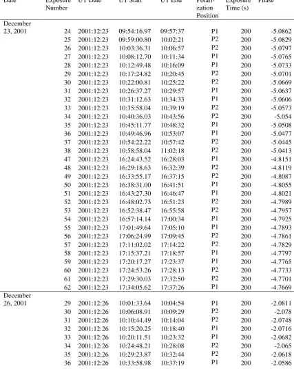
Table 2.2 Log of observations of HR 1817, 23 December 2001 – 2 January 2002. The exposure
numbers are those from the particular night and are not necessarily sequential as other targets were also being observed. The phase is based on a rotational period of 1 day, and zero phase was taken to be approximately half-way though the run. The observations thus spanned over 10 complete rotations of HR 1817. The polarization position refers to the two orthogonal positions of the quarter-wave plate P1 and P2.
Date Exposure Number
UT Date UT Start UT End Polari-zation Position Exposure Time (s) Phase December
23, 2001 24 2001:12:23 09:54:16.97 09:57:37 P1 200 -5.0862 25 2001:12:23 09:59:00.80 10:02:21 P2 200 -5.0829 26 2001:12:23 10:03:36.31 10:06:57 P2 200 -5.0797 27 2001:12:23 10:08:12.70 10:11:34 P1 200 -5.0765 28 2001:12:23 10:12:49.48 10:16:09 P1 200 -5.0733 29 2001:12:23 10:17:24.82 10:20:45 P2 200 -5.0701 30 2001:12:23 10:22:00.81 10:25:22 P2 200 -5.0669 31 2001:12:23 10:26:37.27 10:29:57 P1 200 -5.0637 32 2001:12:23 10:31:12.63 10:34:33 P1 200 -5.0606 33 2001:12:23 10:35:58.04 10:39:19 P2 200 -5.0573 34 2001:12:23 10:40:36.03 10:43:56 P2 200 -5.054 35 2001:12:23 10:45:11.77 10:48:32 P1 200 -5.0508 36 2001:12:23 10:49:46.96 10:53:07 P1 200 -5.0477 37 2001:12:23 10:54:22.22 10:57:42 P2 200 -5.0445 38 2001:12:23 10:58:58.04 11:02:18 P2 200 -5.0413 47 2001:12:23 16:24:43.52 16:28:03 P1 200 -4.8151 48 2001:12:23 16:29:18.63 16:32:39 P2 200 -4.8119 49 2001:12:23 16:33:55.17 16:37:15 P2 200 -4.8087 50 2001:12:23 16:38:31.00 16:41:51 P1 200 -4.8055 51 2001:12:23 16:43:27.30 16:46:47 P1 200 -4.8021 52 2001:12:23 16:48:02.73 16:51:23 P2 200 -4.7989 53 2001:12:23 16:52:38.47 16:55:58 P2 200 -4.7957 54 2001:12:23 16:57:14.14 17:00:34 P1 200 -4.7925 55 2001:12:23 17:01:49.64 17:05:10 P1 200 -4.7893 56 2001:12:23 17:06:24.99 17:09:45 P2 200 -4.7861 57 2001:12:23 17:11:02.02 17:14:22 P2 200 -4.7829 58 2001:12:23 17:15:37.21 17:18:57 P1 200 -4.7797 59 2001:12:23 17:20:17.27 17:23:37 P1 200 -4.7765 60 2001:12:23 17:24:53.26 17:28:13 P2 200 -4.7733 61 2001:12:23 17:29:30.03 17:32:50 P2 200 -4.7701 62 2001:12:23 17:34:05.62 17:37:26 P1 200 -4.7669 December
Date Exposure
Number UT Date UT Start UT End Polari-zation Position
Date Exposure
Number UT Date UT Start UT End Polari-zation Position
Exposure Time (s) Phase 92 2001:12:26 15:21:39.90 15:25:01 P1 200 -1.8589 93 2001:12:26 15:39:14.36 15:42:35 P1 200 -1.8466 94 2001:12:26 15:43:50.99 15:47:11 P2 200 -1.8434 95 2001:12:26 15:48:26.97 15:51:47 P2 200 -1.8403 96 2001:12:26 15:53:02.80 15:56:23 P1 200 -1.8371 101 2001:12:26 16:21:18.86 16:24:39 P1 200 -1.8174 102 2001:12:26 16:25:54.43 16:29:14 P2 200 -1.8142 103 2001:12:26 16:30:30.09 16:33:50 P2 200 -1.811 104 2001:12:26 16:35:06.48 16:38:26 P1 200 -1.8078 105 2001:12:26 16:39:42.29 16:43:02 P1 200 -1.8047 106 2001:12:26 16:44:17.96 16:47:38 P2 200 -1.8015 107 2001:12:26 16:48:53.78 16:52:14 P2 200 -1.7983 108 2001:12:26 16:53:29.85 16:56:50 P1 200 -1.7951 109 2001:12:26 16:58:05.76 17:01:26 P1 200 -1.7919 110 2001:12:26 17:03:01.83 17:06:22 P2 200 -1.7885 111 2001:12:26 17:07:38.14 17:10:58 P2 200 -1.7853 112 2001:12:26 17:12:13.72 17:15:34 P1 200 -1.7821 113 2001:12:26 17:16:50.02 17:20:10 P1 200 -1.7789 114 2001:12:26 17:21:26.01 17:24:46 P2 200 -1.7757 115 2001:12:26 17:26:01.67 17:29:22 P2 200 -1.7725 116 2001:12:26 17:30:46.06 17:34:06 P1 200 -1.7692 December
Date Exposure
Number UT Date UT Start UT End Polari-zation Position
Exposure Time (s) Phase 63 2001:12:30 12:52:26.00 12:55:46 P2 200 2.0375 64 2001:12:30 12:57:01.27 13:00:21 P1 200 2.0407 65 2001:12:30 13:01:36.29 13:04:56 P1 200 2.0439 66 2001:12:30 13:06:11.65 13:09:32 P2 200 2.0471 67 2001:12:30 13:10:46.76 13:14:07 P2 200 2.0503 68 2001:12:30 13:15:28.58 13:18:49 P1 200 2.0535 69 2001:12:30 13:28:40.44 13:32:01 P1 200 2.0627 70 2001:12:30 13:33:16.91 13:36:37 P2 200 2.0659 71 2001:12:30 13:37:52.09 13:41:12 P2 200 2.0691 72 2001:12:30 13:42:27.77 13:45:49 P1 200 2.0723 73 2001:12:30 13:47:04.55 13:50:25 P1 200 2.0755 74 2001:12:30 13:51:41.42 13:55:03 P2 200 2.0787 75 2001:12:30 13:56:18.28 13:59:38 P2 200 2.0819 76 2001:12:30 14:00:54.27 14:04:14 P1 200 2.0851 81 2001:12:30 14:26:21.06 14:29:41 P1 200 2.1027 82 2001:12:30 14:30:56.41 14:34:17 P2 200 2.1059 83 2001:12:30 14:35:33.11 14:38:53 P2 200 2.1091 84 2001:12:30 14:40:08.46 14:43:28 P1 200 2.1123 85 2001:12:30 15:00:35.25 15:03:55 P1 200 2.1265 86 2001:12:30 15:24:09.07 15:27:29 P2 200 2.1429 87 2001:12:30 15:28:44.58 15:32:05 P2 200 2.1461 88 2001:12:30 15:33:21.05 15:36:41 P1 200 2.1493 89 2001:12:30 15:37:56.56 15:41:17 P1 200 2.1525 90 2001:12:30 15:42:33.26 15:45:53 P2 200 2.1557 91 2001:12:30 15:47:09.88 15:50:30 P2 200 2.1589 92 2001:12:30 15:51:48.51 15:55:10 P1 200 2.1621 93 2001:12:30 15:56:29.13 15:59:49 P2 200 2.1653 98 2001:12:30 16:26:25.43 16:29:46 P1 200 2.1861 99 2001:12:30 16:31:02.86 16:34:23 P2 200 2.1893 100 2001:12:30 16:35:38.37 16:38:58 P2 200 2.1925 101 2001:12:30 16:40:13.39 16:43:33 P1 200 2.1957 102 2001:12:30 16:44:49.70 16:48:10 P1 200 2.1989 103 2001:12:30 16:49:30.65 16:52:51 P2 200 2.2022 104 2001:12:30 16:54:06.80 16:57:27 P2 200 2.2053 105 2001:12:30 16:58:43.98 17:03:44 P1 300 2.2086 106 2001:12:30 17:04:59.40 17:08:19 P1 200 2.2129 107 2001:12:30 17:09:35.09 17:12:55 P2 200 2.2161 108 2001:12:30 17:14:11.93 17:17:32 P2 200 2.2193 109 2001:12:30 17:18:47.68 17:22:08 P1 200 2.2225 January 2,
2002 24 2002:01:02 10:24:46.46 10:28:07
P1
Date Exposure
Number UT Date UT Start UT End Polari-zation Position
Exposure Time (s) Phase 32 2002:01:02 11:01:45.79 11:05:06 P1 200 4.9607 33 2002:01:02 11:06:21.31 11:09:41 P2 200 4.9639 34 2002:01:02 11:10:56.82 11:14:17 P2 200 4.967 35 2002:01:02 11:15:33.70 11:18:54 P1 200 4.9702 36 2002:01:02 11:20:10.79 11:23:31 P1 200 4.9735 37 2002:01:02 11:24:46.38 11:28:08 P2 200 4.9766 38 2002:01:02 11:29:23.16 11:32:43 P2 200 4.9798 39 2002:01:02 11:33:58.27 11:37:21 P1 200 4.983 44 2002:01:02 11:59:26.43 12:02:46 P1 200 5.0007 45 2002:01:02 12:04:03.85 12:07:24 P2 200 5.0039 46 2002:01:02 12:08:39.92 12:12:00 P2 200 5.0071 47 2002:01:02 12:13:16.15 12:16:36 P1 200 5.0103 48 2002:01:02 12:17:57.82 12:21:18 P1 200 5.0136 49 2002:01:02 12:22:35.17 12:25:55 P2 200 5.0168 50 2002:01:02 12:27:15.63 12:30:36 P2 200 5.02 51 2002:01:02 12:31:52.11 12:35:12 P1 200 5.0232 52 2002:01:02 12:36:28.82 12:39:49 P1 200 5.0264 53 2002:01:02 12:41:06.27 12:44:26 P2 200 5.0296 54 2002:01:02 12:45:42.79 12:49:03 P2 200 5.0328 55 2002:01:02 12:50:19.02 12:53:39 P1 200 5.036 56 2002:01:02 12:54:56.45 12:58:17 P1 200 5.0393 57 2002:01:02 12:59:33.95 13:02:54 P2 200 5.0425 58 2002:01:02 13:04:09.61 13:07:30 P2 200 5.0457 59 2002:01:02 13:08:46.15 13:12:06 P1 200 5.0489
2.3
Analysis: Spectral Extraction
The raw frames taken using the instrumental setup described in Section 2.1 need to be
converted into wavelength calibrated spectra. To achieve this, a custom-written package
called ESpRIT (Echelle Spectra Reduction: an Interactive Tool) was used. A summary of
the operation of ESpRIT is shown here; a much more detailed description can be found in
Donati et al. (1997). The code base I used is maintained by Jean-François Donati, and he
Why use ESpRIT?
Due to the peculiarities of the instrumental setup used for Zeeman Doppler Imaging,
Donati et al. decided to develop a dedicated package for image extraction. Each order
produced by UCLES include two spectra; one for each polarization state. Also, the use
of the Bowen-Walraven image slicer produces a complicated order section profile. The
slicer also generates distortion in the slit shape. As discussed in Donati et al. (1997) these
peculiarities present difficulties for more conventional data reduction routines.
Because Zeeman Doppler Imaging is searching for very small distortions in
spectral lines, spectral resolution must be as high as possible and the data reduction
process must result in minimal degradation of the quality of the resultant spectra. Also,
the slit tilt and distortion must be taken into account, otherwise it is possible to introduce
spurious polarization signals.
The extraction of the calibrated spectra from raw frames takes 3 steps. Firstly, the
geometrical features of the raw frames are determined. Second, a wavelength calibration
is performed. Finally, the extraction of the intensity and/or polarization spectrum is
performed by an optimal extraction method. Additionally, to eliminate any shifts in the
spectrograph during an observing session, each wavelength calibrated spectrum is shifted
to match the Least-Squared Deconvolved profile of the telluric lines contained in the
spectrum. This reduces any instrumental shift to less than 0.1 km s-1.
Frame Calibration (Geometric)
The geometrical elements of the raw echelle frames are extracted in a process which
overscan and the frames may be mirrored to obtain a standard orientation with orders
running vertically and wavelength increasing along with pixel number. The user
provides an estimate of the location of the centre of the field and the width of the first
order. The ESpRIT code then locates and traces each order in the flat-field frame.
Next, within each order, the spectrum of the arc frame is cross-correlated to trace
the shape of the arc lines perpendicular to the dispersion. A linear or 2D quadratic fit to
these measurements provides a measurement of the slit direction. The deviations from
this mean slit direction averaged across all orders provides an estimate of the slit shape.
Frame Calibration (Wavelength)
Once the geometric characteristics of the raw frames are determined, the user provides an
initial wavelength position and dispersion measurement for the first order. The ESpRIT
code then attempts to calibrate the first selected order; starting with the initial user input
and an atlas of known line positions, the code performs a preliminary identification of
lines which should be present in the selected order. The code then iteratively calibrates
each order. As Donati et al. (1997) mention, the code is very efficient, with mean rms
calibration accuracies better than 0.3 pm (3 mÅ).
The calibration polynomials generated here are then used in the optimal extraction
of the intensity and polarization spectra.
Extraction of Intensity Spectra
For the extraction of intensity spectra, ESpRIT requires the stellar exposure to be
geometric and wavelength calibration processes described above. All frames are
bias-subtracted and the stellar exposure is corrected for pixel-to-pixel sensitivity differences
by dividing each pixel by the corresponding pixel in the flat-field exposure. An estimate
of the inter-order background is obtained from the stellar exposure.
A preliminary spectrum is obtained by collapsing the orders along the slit
direction and shape. At this point pixels which deviate too much from the average
intensity of the order are excluded. This eliminates strong cosmic ray hits on the
detector. The code then generates a false image by propagating the preliminary spectrum
along the slit direction in each order, dividing by the actual stellar image. Marsh’s (1989)
scheme is then applied to give fractional fluxes as a function of the distance from the
centre of the order. Finally, a new optimized spectrum is obtained.
The wavelength calibration is automatically corrected for the heliocentric motion
of the observatory.
Extraction of Polarized Spectra
The extraction of polarized spectra is similar in principle to the intensity spectrum
extraction. As mentioned in Section 3, observations in polarized light consist of a
sequence of four stellar exposures, each of which contain two interleaving spectra
corresponding to the orthogonal polarization states. The first and fourth exposures
correspond to one position of the quarter-wave plate, the second and third corresponding
to the second position. Each individual stellar exposure is processed as for an intensity
Once the four frames (yielding eight spectra) are processed, the mean intensity
spectrum I is derived by adding the spectra. The polarization rate P/I is given by
1 1 + − = R R I P (2.1) where , 3 , 3 , 4 , 4 , 2 , 2 , 1 , 1 4 / / / / i i i i i i i i R ⊥ ⊥ ⊥ ⊥ = (2.2) ⊥ , k
i and ik, being the two spectra obtained from the exposure k. The polarization is thus
obtained by dividing spectra with orthogonal polarization states. This method eliminates
systemic errors and spurious signals that result because both polarization states cannot be
recorded at the same time on the same instrument.
A “null” polarization spectrum, N/I can be obtained be replacing R in equation
(2.1) by , 3 , 3 , 2 , 2 , 4 , 4 , 1 , 1 4 / / / / i i i i i i i i R ⊥ ⊥ ⊥ ⊥ = (2.3)
This is interesting to check that the signature is in fact real. In the case that a
cycle of four exposures is incomplete, a pair of exposures at different positions can still
be used by replacing R in (2.1) by
, 2 , 2 , 1 , 1 2 / / i i i i R ⊥ ⊥
= (2.4)
2.4
Analysis: Least Squares Deconvolution
The Zeeman magnetic signatures that we try to detect are very small; of the order of 0.1%
of the relative amplitude. Even variations in the intensity profiles are small, although at
~ 1% of relative amplitude they are a factor of ten larger than the Zeeman signatures. In
both cases, a high signal-to-noise ratio is required to accurately detect both phenomena.
Donati et al. (1997) indicate that noise levels for the Stokes V profile must be of the order
of 10-4. This is not achievable with a single spectral line within a given spectrum. Also,
co-adding spectra from different phases of the stellar rotation is not an option as the stars
which we observe are rapid rotators and their activity varies on short timescales.
However, we assume the distortions due to spots (in intensity profiles) or
magnetic fields (in Zeeman signatures) in spectral line profiles are the same across every
spectral line in the entire spectrum.
Donati et al. (1997) present a technique called Least Squares Deconvolution
(LSD) which we use to extract the intensity and magnetic information from many lines in
a spectrum and combine them into a single, high-S/N line profile. In addition, due to the
overlap in orders when taking echelle data, some spectral lines are seen twice, and the
LSD technique takes advantage of these duplicate lines. (Note that some very strong
lines such as Balmer lines and Na D are not used).
If the photospheric lines are all affected in the same way by the presence of spots
or a magnetic field, then the observed profile of the lines is a convolution of a basic line
pattern (M) and the spot signature (Z). The observed intensity profile (I) can thus be
expressed as:
Z M
Similarly, the observed circularly polarized spectrum V can be expressed:
Z M
V = ∗ (2.6)
where M is a line mask. Masks of various stellar atmospheres from A0 to M0 have been
computed using the Kurucz’s atomic database (Kurucz, 1993).
Solving for Z by a least-squares method results in:
I S M M S M
Z =(