Apan, A., Datt, B., and Kelly, R. Detection of Pests and Diseases in Vegetable Crops Using Hyperspectral Sensing: A Comparison of Reflectance Data for Different Sets of Symptoms. Proceedings of SSC 2005 Spatial Intelligence, Innovation and Praxis: The national biennial
Conference of the Spatial Sciences Institute, September 2005. Melbourne: Spatial Sciences Institute. ISBN 0-9581366-2-9
DETECTION OF PESTS AND DISEASES IN VEGETABLE CROPS
USING HYPERSPECTRAL SENSING: A COMPARISON OF
REFLECTANCE DATA FOR DIFFERENT SETS OF SYMPTOMS
A. Apan
1, B. Datt
2, and R. Kelly
31
Geospatial Information and Remote Sensing Group, Faculty of Engineering and Surveying,
University of Southern Queensland, Toowoomba 4350 QLD Australia, Phone: +61 7 4631-1386,
Fax: +61 7 4631-2526
2
CSIRO Exploration and Mining, PO Box 136, North Ryde, NSW 1670, Phone: + 61 2 9490-8884,
Fax: +61 2 9490-8960
3
Plant Science, Queensland Department of Primary Industries and Fisheries, Toowoomba 4350
QLD Australia, Phone: + 61 7 4688-1524, Fax: +61 7 4688-1809
KEYWORDS:
hyperspectral sensing, pests and diseases, vegetables, PLS regression
ABSTRACT
The aim of the study was to examine the potential of hyperspectral sensing to detect the incidence of pests and diseases in vegetable crops. The specific objectives were: a) to test if symptoms of pests and diseases of vegetable crops can be detected by hyperspectral sensing, b) to determine the best spectral bands relevant to pest and disease detection, and c) to compare the spectral responses obtained from the symptoms of two different pest and disease. Using a handheld spectrometer, sample measurements of diseased/infested and healthy leaves were collected separately from tomato and eggplant crops. The tomato crops were affected by a fungal “early blight” disease (Alternaria solani), with symptoms characterised by a yellowing or chlorosis of leaves. Conversely, the eggplants exhibited skeletal interveinal damage (“holes”) on leaves, caused by the 28-spotted ladybird (Epilachna vigintioctopunctata). To overcome the problems of using traditional regression techniques, the Partial Least Squares (PLS) regression technique was used.
The cross-validated results showed that the incidence of disease on tomato and pest on eggplant could be predicted with 82% accuracy. Different sets of symptoms (i.e. chlorosis vs. loss of leaf area) provided different sets of optimum number of principal components and significant predictor variables. The most significant spectral bands for the tomato disease prediction corresponded to the reflectance red-edge (690nm-720nm), as well as the visible region ( 400nm-700nm), and part of near-infrared wavelengths (735nm-1142nm). For the eggplant, the near-infrared region (particularly the bands 732nm-829nm) was identified by the regression model to be as equally significant as the red-edge ( 694nm-716nm) in the prediction. However, the inclusion of the shortwave infrared bands (1590nm-1766nm) as significant variables in the eggplant regression model has indicated the contributing role of other factors. Results such as these confirmed the utility of hyperspectral data to diagnose pests and diseases of vegetables that can improve detection speed and provide opportunity for non-destructive sampling.
BIOGRAPHY OF PRESENTER
INTRODUCTION
Pests and diseases cause serious economic losses in yield and quality of cultivated plants [Tatchell, 1989; Walker, 1983; MacLeod, et al, 2004]. Thus, the detection and assessment of their symptoms is essential in commercial agriculture. Traditionally, disease and pest damage assessment in plant populations is being done by visual approach, i.e. relying upon the human eye and brain to assess the incidence of disease or pest in crops. However, the problem with the traditional approaches is that they are often time-consuming and labour intensive [Lucas, 1998, p. 54]. Therefore, there is a need to develop different approaches that can enhance or supplement traditional techniques.
Remote sensing has been used in agriculture for many decades [see, for example, the review of Moran, et al., 1997]. One of its earliest applications was on crop disease assessment. Reflectance data was found to be capable of detecting changes in the biophysical properties of plant leaf and canopy associated with pathogens and insect pests. Additionally, remote sensing may provide a better means to objectively quantify disease stress than visual assessment methods, and it can be used to repeatedly collect sample measurements non-destructively and non-invasively.
Hyperspectral sensing, a technique that utilises sensors operating in hundreds of narrow contiguous spectral bands, offers potential to improve the assessment of crop diseases and pests. While its application to pest and disease detection is not new, however, the comparative assessment of two different sets of symptoms brought by a pathogen and an insect has rarely been conducted. Therefore, the aim of the study was to comparatively examine the level and nature of detection of two different sets of symptoms of pests and diseases in vegetable crops using hyperspectral sensing. The specific objectives were: a) to test if the two symptoms of pests and diseases of vegetable crops can be adequately detected by hyperspectral sensing, b) to determine the best spectral bands relevant to pest and disease detection, and c) to compare the spectral responses obtained from the symptoms of two different pest and disease.
REMOTE SENSING OF PESTS AND DISEASES IN CROPS
Studies on the use of remote sensing for crop disease assessment started long time ago. For example, in the late 1920s, aerial photography was used in detecting cotton root rot [Taubenhaus et. al., 1929]. The use of infrared photographs was first reported in determining the prevalence of certain cereal crop diseases [Colwell, 1956]. In the early 1980s, Toler, et al., [1981] used aerial colour infrared photography to detect root rot of cotton and wheat stem rust. In these studies, airborne cameras were used to record the reflected electromagnetic energy on analogue films covering broad spectral bands. Since then, remote sensing technology has changed significantly. Satellite based imaging sensors, equipped with improved spatial, spectral and radiometric resolutions, offer enhanced capabilities over those of previous systems.
Pathogens and pests can induce physiological stresses and physical changes in plants, such as chlorosis or yellowing (reduction in plant pigment), necrosis (damage on cells), abnormal growth, wilting, stunting, leaf curling, etc. [Nutter and Gaunt, 1996]. Incidentally, these changes can alter the reflectance properties of plants. In the visible portion of the electromagnetic spectrum (approx. 400nm to 700nm), the reflectance of green healthy vegetation is relatively low due to strong absorption by pigments (e.g. chlorophyll) in plant leaves. If there is a reduction in pigments due to pests or diseases, the reflectance in this spectral region will increase. Vigier et al. [2004] found that reflectance in the red wavelengths (e.g. 675–685nm) contributed the most in the detection of sclerotinia stem rot infection in soybeans.
At about 700nm to 1300nm (i.e. the near-infrared portion (NIR)), the reflection of healthy vegetation is significantly high. With a disease or pest that damaged the leaves (e.g. cell collapse), the overall reflectance in the NIR region is expected to be lower. Ausmus and Hilty [1972], in their study of maize dwarf mosaic virus, concluded that the NIR wavelengths were useful in reflectance studies of crop disease. On stress in tomatoes induced by late blight disease, it was found that the near-infrared region, was much more valuable than the visible range to detect disease [Zhang, et al., 2003]. In a different spectral region of the shortwave infrared (SWIR) range (1300nm to 2500µm), the spectral properties of vegetation are dominated by water absorption bands. Less water on leaves and canopies will increase reflectance in this region. Apan et al. [2005] noted the key role of the SWIR narrowbands in the spectral discrimination of healthy and diseased (orange rust) sugarcane crops.
RESEARCH METHODS
Study Area, Crop Attributes and Data Acquisition
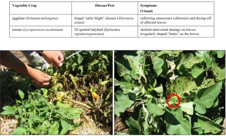
[image:3.612.77.540.211.490.2]The study area is located near Toowoomba, Queensland, Australia. With sub-tropical climate, the site is part of a small-scale (approx. 0.25 ha) organic, pesticide-free garden of various vegetable crops. The tomato crops were affected by a fungal “early blight” disease (Alternaria solani), with symptoms characterised by a yellowing senescence (chlorosis) and drying-off of the affected leaves (Table 1 and Figure 1). Conversely, the eggplants exhibited skeletal interveinal damage on mostly older leaves that created irregularly shaped “holes”. These symptoms were characteristic of leaf damage caused by the 28-spotted ladybird (Epilachna vigintioctopunctata).
Table 1. Vegetable crops and pest and diseases in the study
Vegetable Crop Disease/Pest Symptoms
(Visual)
eggplant (Solanum melongena) fungal “early blight” disease (Alternaria solani)
yellowing senescence (chlorosis) and drying-off of affected leaves
tomato (Lycopersicon esculentum) 28-spotted ladybird (Epilachna vigintioctopunctata)
skeletal interveinal damage on leaves; irregularly shaped “holes” on the leaves
Figure 1. From left: (a) tomato plant with fungal “early blight” disease and (b) eggplant with a pest “28-spotted ladybird” (encircled)
Using a handheld ASD FieldSpec Pro FR spectrometer [Analytical Spectral Devices, 2002] operating in the 350nm to 2500nm range, sample measurements of diseased/infested and non-diseased/non-infested leaves were collected separately from the tomato and eggplant crops. Following the sampling procedures and considerations provided in the User’s Guide, each sample corresponded to a field of view of about 1.5 cm diameter, collected between 1030 to 1200 hr on 10th February 2005. While there was no ordinal measurement scale used to categorise disease severity, the
“diseased” or “insect-infested” samples were taken from leaves where symptoms are visually obvious.
Data Pre-processing and Analysis
Graphical plots of the spectra were examined to check for potential erroneous samples, as well as to initially explore the nature and magnitude of the differences between sample measurements. “Noisy” bands (covering the spectral ranges 325-399nm, 1356 – 1480 nm, 1791 – 2021 nm and greater than 2396 nm) were removed and thus excluded from the analysis.
of several predictors (X-variables), with explanatory or predictive purposes [Esbensen, 2002]. Unlike the classical multiple regression technique, PLS performs particularly well when the various X-variables have high correlation (which is often the case for hyperspectral data). Information in the original X-data is projected onto a small number of underlying (“latent”) variables called PLS components.
Aside from the raw reflectance data, its first derivative was also calculated and analysed using the full the cross-validation (leave-one-out) technique. The root mean error of prediction (RMSEP) was calculated, which gave the measurement of the average difference between predicted and measured response values. It can be interpreted as the average prediction error, expressed in the same unit as the original response value [CAMO, 2004]. The RMSEP values between datasets can be compared to determine which PLS regression model is better than others.
RESULTS AND DISCUSSION
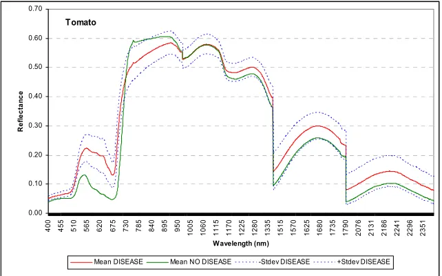
[image:4.612.146.467.321.521.2]The mean reflectance values of diseased samples in tomato showed good spectral separability over the healthy ones (Figure 2). In the visible green and red region, the absolute mean difference values were highest from 545nm to 700nm wavelengths (Figure 3). Selected portion of the NIR region (730nm-800nm) also showed good separation for the diseased and healthy samples. However, it was the red-edge sub-region (690-720nm) that displayed the highest absolute difference for all the spectral regions (Figure 3), indicating its importance in discriminating diseased and non-diseased samples. Since chlorosis is the dominant symptom of the diseased leaves in tomato, red-edge’s sensitivity to loss of chlorophyll was demonstrated here. This agreed with previous studies that found the red-edge region as a good estimator of chlorophyll-related stress [e.g. Curran, et al. 1995].
Tomato
0.00 0.10 0.20 0.30 0.40 0.50 0.60 0.70
40
0
45
5
51
0
56
5
62
0
67
5
73
0
78
5
84
0
89
5
95
0
100
5
106
0
111
5
117
0
122
5
128
0
133
5
151
5
157
0
162
5
168
0
173
5
179
0
207
6
213
1
218
6
224
1
229
6
235
1
Wavelength (nm)
R
e
fl
e
c
ta
n
c
e
Mean DISEASE Mean NO DISEASE -Stdev DISEASE +Stdev DISEASE
Tomato 0 0.02 0.04 0.06 0.08 0.1 0.12 0.14 0.16 0.18 0.2
400 466 532 598 664 730 796 862 928 994 1060 1126 1192 1258 1324 1515 1581 1647 1713 1779 2076 2142 2208 2274 2340
Wavelength Di ff er en ce o f M ean D iseased an d No n -D iseased ( A b so lu te V al u e)
[image:5.612.144.468.68.286.2]ABS(MeanDisease - MeanNoDisease) red-edge
Figure 3. Absolute difference of mean diseased and non-diseased values (tomato)
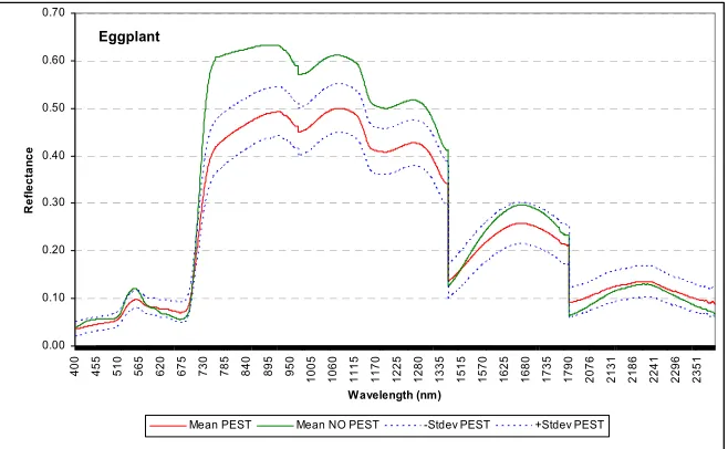
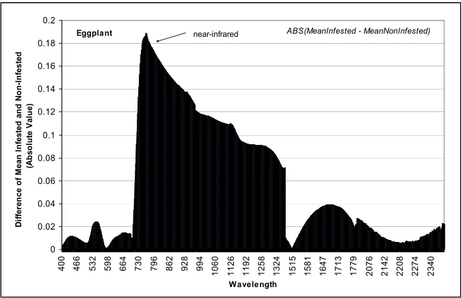
For the eggplant, the mean reflectance values of infested and non-infested samples also showed good spectral separability (Figure 4). The difference in the red-edge sub-region was also high. However, unlike the tomato crop, the eggplant’s mean difference values were highest in the near-infrared region, i.e. from 720nm to 1300nm. Furthermore, there is a relatively big difference in the mean reflectance values in the shortwave infra-red (SWIR) region, particularly at the range 1590nm-1766nm (peak at 1660nm) (Figure 5). The significance of the near-infrared wavelengths in this case concurred with the knowledge that the NIR region decreases when there is a loss of leaf area, foliage density, and other changes in canopy characteristics [e.g. Kollenkark et al., 1982; Gausman, 1974]. For the SWIR region, the lower reflectance of infested samples did not necessarily indicate that there is more water on these leaves than the healthy ones. This lower reflectance may be due to the contributing reflectance of black moist soil under the plant canopy, shadow, and other plant components. The “holes” on the leaves may have allowed the capture of reflectance from these materials. Eggplant 0.00 0.10 0.20 0.30 0.40 0.50 0.60 0.70 40 0 45 5 51 0 56 5 62 0 67 5 73 0 78 5 84 0 89 5 95 0 100 5 106 0 111 5 117 0 122 5 128 0 133 5 151 5 157 0 162 5 168 0 173 5 179 0 207 6 213 1 218 6 224 1 229 6 235 1 Wavelength (nm) R ef lect an c e
Mean PEST Mean NO PEST -Stdev PEST +Stdev PEST
[image:5.612.143.472.452.655.2]Eggplant
0 0.02 0.04 0.06 0.08 0.1 0.12 0.14 0.16 0.18 0.2
400 466 532 598 664 730 796 862 928 994 1060 1126 1192 1258 1324 1515 1581 1647 1713 1779 2076 2142 2208 2274 2340 Wavelength
D
if
fer
en
ce o
f M
ean
I
n
fest
ed
an
d
No
n
-I
n
fes
ted
(A
b
so
lu
te
V
al
u
e)
[image:6.612.137.474.67.285.2]near-infrared ABS(MeanInfested - MeanNonInfested)
Figure 5. Absolute difference of mean infested and non-infested values (eggplant)
The PLS regression results showed that it is possible to predict the incidence of pest and disease on vegetable crops using hyperspectral data. There is a high correlation (r=0.90 to 0.98) between predicted and measured values for the calibrated and validated samples (Table 2). The root mean square error of calibration (RMSEC) and prediction (RMSEP) were relatively low (from 18-21%), indicative of the good prediction accuracy of the regression models. For both crops, the first derivative of the spectra provided a slight increase in the prediction accuracy compared with the raw spectra, i.e. from 79% to 82%.
For the tomato, the optimal number of PLS factors (components) was minimal (i.e. two for the raw spectra and one for the first derivative data), but was able to explain the Y-variance fairly sufficiently (i.e. from 82.5% to 86.9%). The score plot in Figure 6a has also indicated that there is a good separation with the disease (“YES”) and without disease (“NO”) samples in the first two principal components. This is desirable — ideally, one would like to have simple models, where the total explained variance goes to 100% with as few components as possible. In contrast, the eggplant model needed three to four components to attain similar percentage of Y-variance (Table 2). It may mean that there is a set, or other sets, of structured information inherent in the data. In the score plot (Figure 7a), the separation or “clustering” of the eggplant data in the first two components is not as good as in the tomato samples. The third and fourth components are needed for the eggplant data.
Table 2. PLS Regression Results of Vegetable Pest and Disease and Reflectance Values Calibration Cross-Validation
(leave-one-out)
Data Optimal no.
of PLS
factors R* RMSEC**
value
R* RMSEP*** value
Prediction Accuracy %
% of Y Variance Explained TOMATO (n=33)
1. Raw spectra 2 0.92 0.19 0.90 0.21 79 82.5
2. First derivative 1 0.94 0.17 0.93 0.18 82 86.9
EGGPLANT (n=31)
1. Raw spectra 4 0.95 0.16 0.90 0.20 80 83.5
2. First derivative 3 0.98 0.09 0.93 0.18 82 87.1
[image:6.612.89.526.522.630.2]-2.0 -1.5 -1.0 -0.5 0 0.5 1.0 1.5
-3.0 -2.5 -2.0 -1.5 -1.0 -0.5 0 0.5 1.0 1.5
RESULT_TOMATO_3…, X-expl: 54%,22% Y-expl: 72%,13%
YES YES YES YES YES YES YES YES YES YES YES YES YES NO NO NO NO NO NO NO NO NO NO NO NO NO NO NO NO NO NO NO NO PC1 PC2 Scores -0.05 -0.04 -0.03 -0.02 -0.01 0 0.01 0.02 40
0 582 764 946 1128 1310 1617 2030 2212 2394
RESULT_TOMATO_3…, (Y-var, PC): (CODE,2) B0 = -0.391552
1
X1-Variables Raw Regression Coefficients [B0]
Figure 6. (a) Score plot of tomato reflectance samples with disease (“YES”) and without disease (“NO”), in the first two principal components, (b) regression coefficients for the cross-calibrated prediction model involving disease and raw reflectance data. The higher
the value of a coefficient, the more significant it is in the prediction model.
-2.0 -1.5 -1.0 -0.5 0 0.5 1.0 1.5
-4 -3 -2 -1 0 1 2 3 4
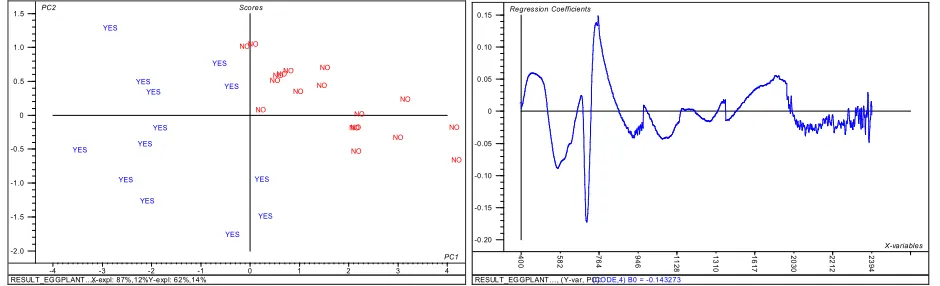
RESULT_EGGPLANT…, X-expl: 87%,12% Y-expl: 62%,14%
YES YES YES YES YES YES YES YES YES YES YES YES YES NO NO NO NO NO NO NO NO NO NO NO NO NO NO NO NO NO NO PC1 PC2 Scores -0.20 -0.15 -0.10 -0.05 0 0.05 0.10 0.15 40 0 58 2 76 4 94 6 11 28 13 10 16 17 20 30 22 12 23 94
RESULT_EGGPLANT…, (Y-var, PC): (CODE,4) B0 = -0.143273
1
X-variables Regression Coefficients
Figure 7. (a) Score plot of eggplant reflectance samples with pest (“YES”) and without pest (“NO”), in the first two principal components, (b) regression coefficients for the cross-calibrated prediction model involving disease and raw reflectance data. The higher the value of a
coefficient, the more significant it is in the prediction model.
Based on the regression coefficient plots (Figure 6b) and by the results of Martens’ Uncertainty Test, the most significant spectral bands for the tomato disease prediction corresponded to the reflectance red-edge (690nm-720nm), as well as the visible region (400nm-700nm) and part of near-infrared wavelengths (735nm-1142nm). This is consistent with the results presented earlier using the plots and charts. For the eggplant, the near-infrared region (particularly the bands 732nm-829nm) was identified by the regression model to be as equally significant as the red-edge ( 694nm-716nm) (Figure 7b). However, the inclusion of the shortwave infrared bands (1590nm-1766nm) as significant variables has indicated the contributing role of other factors. As previously hypothesised, the “holes” on the leaves may have allowed the capture of reflectance from soil, shadow and other plant materials.
[image:7.612.74.542.65.213.2] [image:7.612.78.548.273.416.2]CONCLUSIONS
This study demonstrated that it is feasible to detect the effects of insect pest and disease in vegetable crops using hyperspectral measurements. Different sets of pest and disease symptoms provided different sets of diagnostic spectral regions. The most significant spectral bands for the tomato disease prediction corresponded to the reflectance red-edge, as well as the visible region and part of infrared wavelengths. For the eggplant’s insect infestation, the near-infrared region was identified by the regression model to be as equally significant as the red-edge in the prediction. However, the inclusion of the shortwave infrared bands as significant variables has indicated the effect of other contributing factors.
It was recognised in this project that the use of a portable field spectrometer can provide a means for rapid observation and digital recording of hundreds of plant samples in a few hours of scouting through the fields. Combined with Global Positioning Systems (GPS) location data collected simultaneously, field level maps can be created by spatial interpolation among the sampling points. By creating spectral libraries of specific crops comprising a wide range of healthy and diseased crop spectra, such site-specific crop data can be used routinely with various spectral-matching type algorithms for automated detection of disease spots. More work is being done to test other analytical techniques (e.g. SIMCA) to substantiate the results obtained in this study, as well as to analyse the data collected from other vegetable crops with disease severity ratings.
ACKNOWLEDGEMENTS
We thank Rural Industries Research and Development Corporation (RIRDC) for the funding support provided in this project. Tek Maraseni (USQ) provided valuable help during fieldwork. We also appreciate the help of John Duff (DPI&F at Gatton), Anne Story (Story Fresh), Ashley Hannam (Story Fresh), Lester Hamblin (Westview Gardens), Andrew Millers (Westview Gardens), and Murray (Cotswold Hills), for permitting access to the study sites.
REFERENCES
Analytical Spectral Devices (2002), Spectroradiometer User’s Guide, Boulder CO: Analytical Spectral Devices.
Apan, A., Held, A., Phinn, S, and Markley, J., (2004), “Detecting Sugarcane ‘Orange Rust’ Disease Using EO-1 Hyperion Hyperspectral Imagery”, International Journal of Remote Sensing, 25 (2), 489-498.
Ausmus, B.S. and Hilty, J.W. (1972), “Reflectance studies of healthy, maize dwarf mosaic virus-infected, and
Helminthosporium maydis-infected corn leaves”, Remote Sensing of Environment, 2, 77-81.
CAMO (2004), The Unscrambler 9.1, Oslo: CAMO Process AS.
Colwell, J.E. (1956), “Determining the prevalence of certain cereal crop diseases by means of aerial photography”,
Hilgardia, 26, 223-286.
Curran P.J., Windham W.R., Gholz H.L. (1995), “Exploring the relationship between reflectance red edge and chlorophyll concentration in slash pine leaves”, Tree Physiology, 15: 203–206.
Esbensen, K. (2002), Multivariate Data Analysis – in practice, Oslo: CAMO Process AS.
Gausman H. W. (1974), “Leaf reflectance of near infrared”, Photogrammetric Engineering and Remote Sensing, 40, 57-62.
Kollenkark, J.C., Daughtry, C.S.T., Bauer, M.E., and Housley, T.L. (1982), “Effects of cultural practices on agronomic and reflectance characteristics of soybean canopies”, Agronomy Journal, 74, 751-758.
Lucas, J.A. (1998), Plant Pathology and Plant Pathogens, 3rd ed., Oxford: Blackwell Science.
MacLeod, A., Head, J. and Gaunt, A. (2004). “An assessment of the potential economic impact of Thrips palmi on horticulture in England and the significance of a successful eradication campaign”, Crop Protection, 23 (7), 601-610.
Moran, M.S., Inoue, Y., and Barnes, E.M. (1997), “Opportunities and Limitations for Image-Based Remote Sensing in Precision Crop Management”, Remote Sensing of Environment, 61, 319-346.
Nillson, H.E. (1995), “Remote sensing and image analysis in plant pathology”, Annual Review in Phytopathology, 15, 489-527.
Nutter, F.W. Jr and Gaunt, R.E. (1996), “Recent developments in methods for assessing disease losses in forage/pasture crops”, in: Chakraborty, S., Leath, D.T., Skipp, R.A., Pederson, G.A., Barry, R.A., Latch, G.C.M., Nutter, F.W. Jr (Eds), Pasture and Forage Crop Pathology, American Society of Agronomy, Crop Science Society of America, and Soil Science Society of America, Madison, W.I., pp. 93-118.
Tatchell, G. M. (1989), “An estimate of the potential economic losses to some crops due to aphids in Britain”, Crop Protection, 8 (1), 25-29.
Taubenhaus, J.J., Ezekiel, W.N., and Neblette, C.B. (1929), “Airplane photography in the study of cotton root rot”,
Phytopathology, 19, 1025-1029.
Toler, R.W., Smith, B.D., and Harlan, J.C. (1981), “Use of aerial color infrared photography to evaluate crop disease”,
Plant Disease, 65, 24-31.
Vigier, B.J., Pattey, E. and Strachan, I.B. (2004), “Narrowband Vegetation Indexes and Detection of Disease Damage in Soybeans”, IEEE Geoscience and Remote Sensing Letters, 1 (4), 255-259.
Walker, P. T. (1983), “Crop losses: The need to quantify the effects of pests, diseases and weeds on agricultural production”, Agriculture, Ecosystems & Environment, 9 (2), 119-158.