University o f Southern Queensland
FACULTY OF ENGINEERING AND SURVEYING
Bachelor of Engineering Thesis
PID TUNING CONTROLLER
USING
INTERNAL MODEL CONTROL METHOD
PREPARED BY:
Donald A. Mohutsiwa
Bachelor of Engineering (Instrumentation and Control)
In fulfil ment of Course:
ENG 4111/4112 Research Project
Abstract
There are three design methods commonly used nowadays for second order systems, the method of state space design, lag/lead filter compensation and finally the Internal Model Control (IMC) method [3, 8, 11]. The latter design is utilised in control of current in DC electrical motors (servo system) and many other second order systems. The internal model control design has capabilities of achieving high performance. The IMC technique, in theory, substitutes the closed loop system with a low-pass filter of the same order as the system itself. In this case the plant (process) under control is always second order, so if an exact representation of the plant (process model) is given, the step response for a change in the reference signal would look as a low-pass filter step response.
In practice, however, process-model mismatch is common [1,2,3], that is to say designers never achieve a 100% accurate model, and thus IMC method is usually chosen and implemented in the control design scheme. Even if the tracking of the reference input is adequate, most control systems are subjected to disturbances, and IMC is not only designed to optimally suppress these effects, it also tells us that its strategy and concepts that it embraces are clearly very powerful techniques.
The conventional IMC method often involves inversion of a process, which is often difficult or totally impossible [3, 4]. In other words the potential to achieve perfect control with model-based design is dependent on constraints with process operations. Therefore models which will contain some degree of error or to some extent cannot be invertible results in perfect control not being realised. However, for the purpose of control strategy specification, controller design and control system analysis, models that can replicate the dynamic trends of the target processes are usually sufficient. The internal model control scheme has been widely applied in the field of process control. This is due to its simple and straightforward controller design procedure as well as its good disturbance rejection capabilities and robustness properties.
In practice, the tuning of conventional PID controllers can be very time consuming [2, 16], as the effect of the controller coefficients on the control performance cannot be easily described. In addition, the optimization of controller parameters based on the predefined fitness functions is computationally expensive and the design of this fitness functions is difficult because of the involved tuning parameters. In IMC schemes a controller is designed in series with a low pass filter and utilization of this design method means that a controller design involves tuning only one parameter, namely the filter constant. From that, the corresponding parameters of the
Certificate
I certify that the ideas, methods, simulations and planning in this case study are the work of my own. In this thesis, it is important to have specified relevant material in this form of documentation as has been done solely to note areas of related work and concepts. It has been specified that extensive work in this study has been done by quite a large number of disciplines and as acknowledged, I have to certify the importance of their work to help build the ideas of mine.
Donald A. Mohutsiwa
Student No: 0031234287
Signature
:
_________________Date
:
_________________Acknowledgements
CONTENTS
ABSTRACT ...I
CERTIFICATE ... III
ACKN OWLEDGEME NTS...IV
CONTENTS... V
LIST OF FIGURES ... VII
1.0 CHAPTER ONE: INTRODUCTION...1
1.1 INTRODUCTION ...1
1.2 OBJECTIVE...2
1.3 CHAPTER MODULES ...2
1.3.1CHAPTER ONE...3
1.3.2CHAPTER TWO...3
1.3.3CHAPTER THREE...3
1.3.4CHAPTER FOUR...3
1.3.5CHAPTER FIVE...3
1.3.6CHAPTER SIX...3
1.3.7CHAPTER SEVEN...3
1.3.8CHAPTER EIGHT...4
2.0 CHAPTER TWO: INTERNAL MODEL CONTROL...5
2.1 LITERATURE REVIEW ...5
2.2 INTERNAL MODEL CONTROL PRINCIPLE ...5
2.3 INTERNAL MODEL CONTROL PROPERTIES ...8
2.3.1TRANS FER FUNCTIONS...8
2.3.2NO OFFS ET PR OPERTY OF IMC...10
2.3.3PERFECT CONTR OL...10
2.4 DESIGNING FOR IMC ...10
2.4.1PRACTICAL DESIGN OF IMC...11
2.4.2IMCFILTER DESIGN...12
2.5 IMC APPLICATIONS...13
3.0 CHAPTER THREE: SERVO SYSTEM AND MODELLING ...14
3.1 SERVO BACKGROUND...14
3.1.1OVERVIEW...14
3.1.2MATHEM ATICAL MOD EL...15
3.2 SERVO SYSTEM CONTROLLERS ...17
4.0 CHAPTER FOUR: PID CONTROL FOR THE SERVO SYSTEM...18
4.1 INTRODUCTION TO PID CONTROLLERS ...18
4.2 PID MATHEMATICAL REPRESENTATION ...18
4.3.3DERIVATIVE COMM AND...20
4.4 PID DESIGN FOR THE SERVO SYSTEM ...21
4.5 DISTURBANCE EFFECTS WITH PID DESIGN...26
4.5.1STEP INPUT DISTURBANCE AT THE INPUT OF THE PLANT...26
4.5.2SIN USOIDAL DISTURBANCE AT THE INPUT OF THE PLANT...28
4.5.3STEP INPUT DISTURBANCE AT THE OUTPUT OF THE PLANT...29
4.5.4SIN USOIDAL DISTURBANCE AT THE OUTPUT OF THE PLANT...30
4.6 SIMULINK IMPLEMENTATIONS ...33
4.7 RESULTS AND ANALYS IS...33
5.0 CHAPTER FIVE: IMC DESIGN FOR THE SERVO SYSTEM ...34
5.1 IMC CONTROLLER ...34
5.2 FILTER DESIGN FOR THE SERVO SYSTEM ...34
5.3 DISTURBANCE EFFECTS ON THE SERVO SYSTEM ...38
5.3.1STEP INPUT DISTURB ANCE AT THE INPUT OF THE PLAN T...38
5.3.2SIN USOIDAL IN PUT D IS TURBANCE AT THE INPUT OF THE PLANT...40
5.3.3STEP INPUT DISTURB ANCE AT THE OUTPUT OF THE P LANT...42
5.3.2SIN USOIDAL DISTURBANCE AT THE INPUT OF THE PLANT...43
5.4 PLANT- MODEL MISMATCHING ...44
5.4.1GAINVARIATION...45
5.4.2DAM PING FACTOR VARIATION...45
5.4.3CHANGE IN POLE POSITION...46
5.4.3a Model with Stable Complex Poles...46
5.4.3b Model with Unstable Complex Poles...46
5.4.3c Model with Imaginary Axis Poles...46
5.5 SIMULINK IMPLEMENTATIONS ...46
5.6 RESULTS AND ANALYS IS...47
6.0 CHAPTER SIX: IMC-PID FRAMEWORK...48
6.1 IMC-PID PARAMETER SETTING ...48
6.2 IMC-PID PARAMETER TUNING ...53
6.3 SIMULINK IMPLEMENTATIONS ...53
6.4 RESULTS AND ANALYS IS...54
7.0 CHAPTER SEVEN: IMC AND PID COMPARISON ...55
7.1 EFFECTS OF DISTURBANCES ...55
7.2 PARAMETER TUNING ...56
8.0 CHAPTER EIGHT: FUTURE WORK ...57
REFERENCES ...58
APPENDIXA...68
APPENDIXB...70
APPENDIXC...71
APPENDIXE...77
LIST OF FIGURES
FIGURE 2:IN TERNAL MO DEL CONTROL SCHEME...7FIGURE 3:ALTERNATE DESIGN OF IMC SCHEM E...9
FIGURE 4:IMCSCHEM E WITH A FILTER...12
FIGURE 4.1:PROPORTIONAL-INTEGRAL-DERIVATIVE (PID) CONTROLLER...18
FIGURE 4.2:PROPORTIONAL CON TROL...19
FIGURE 4.3:IN TEGR AL CON TROL...20
FIGURE 4.4:DERIVATIVE CONTROL...20
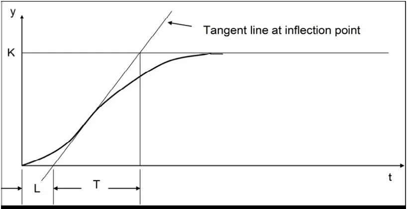
FIGURE 4.5:AN S-SHAPED OPEN LOOP R ESPONS E OF A S YSTEM...22
FIGURE 4.6:OPEN LOOP RESPONS E TO A STEP INPUT FOR ZIEGLER-NICHOLS FIRS T TRIAL...24
FIGURE 4.7:PID CONTR OL-ZN FIRS T TRIAL...25
FIGURE 4.8:PID CONTR OL-ZNSECOND TR AIL...26
FIGURE 4.9:PID CONTR OL UNDER A S TEP D IS TURBAN CE AT INPUT OF PLAN T...27
FIGURE 4.10:PID CONTROL UNDER A SINUSOID AL DISTURBANCE AT IN PUT OF PLANT...28
FIGURE 4.11:PID CONTROL WITH S TEP IN PUT D IS TURB ANCE AT OUTPUT OF PLANT...29
FIGURE 4.12:PID CONTROL WITH A S IN USOIDAL DISTURBANCE AT THE OUTPUT OF PLAN T...30
FIGURE 5.1:RES PONS E TO A S TEP INPUT WITH IMC CONTR OLLER...37
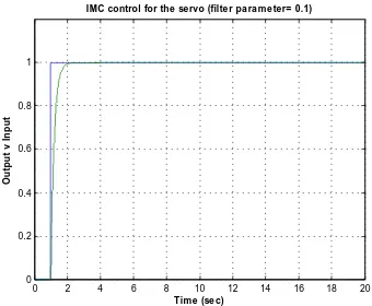
FIGURE 5.2:IMC CON TROL-FILTER PARAMETER=0.1...38
FIGURE 5.3:IMC CON TROL WITH STEP DIS TUR BAN CE AT PLAN T INPUT...39
FIGURE 5.4:IMC CON TROL WITH SIN USOIDAL DISTURBANCE AT PLANT IN PUT (F =0.01)...41
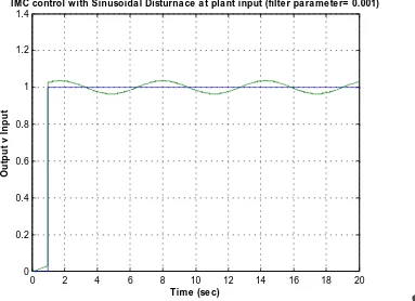
FIGURE 5.5:IMC CON TROL WITH SIN USOIDAL DISTURBANCE AT PLANT IN PUT (F =0.001)...41
FIGURE 5.6:IMC CON TROL WITH A STEP DIS TURBAN CE AT PLAN T IN PUT (F =0.1)...42
FIGURE 5.6:IMC CON TROL WITH A SIN USOIDAL DISTURBANCE AT PLANT OUTPUT (F =0.1)...43
FIGURE 5.7:IMC CON TROL WITH SIN USOIDAL DISTURBANCE AT PLANT OUTPUT (
F =0.001)....44FIGURE 5A.2:PROCESS-MOD EL MISM ATCH (GAIN=1)...62
FIGURE 5A.3:PROCESS-MODEL MISM ATCH (GAIN=200)...63
FIGURE 5A.4:REDUCTION IN DAM PIN G IN THE MODEL...64
FIGURE 5A.5:IN CREASE IN DAM PIN G IN THE MODEL...65
FIGURE 5A.6:MODEL WITH STAB LE COMPLEX POLES...66
FIGURE 5A.7:MODEL WITH UNSTABLE COM PLEX POLES...67
FIGURE 5A.8:MODEL WITH POLES ON THE IM AGIN ARY AXIS...68
FIGURE 6C.1:IMC-PID(STEP DISTURBANCE AT IN PUT OF PLANT)...71
FIGURE 6C.2:IMC-PID(STEP DISTURBANCE AT OUTPUT OF PLAN T)...72
FIGURE 6C.3:IMC-PID(STEP AT BOTH INPUT &OUTPUT OF PLAN T)...73
FIGURE 6C.4:IMC-PID(SINE DISTURB ANCE AT INPUT OF THE PLAN T)...74
1.0 Chapter One: Introduction
1.1 Introduction
In theory, control systems can be condensed into a simple set of tasks- measure your system, make a decision based on the input, send a control signal to adjust your system to expected operation, and then repeat. In reality or so to say in practice, accomplishing each of these tasks can grow a lot more complex in many ways [12], once you take into account the types of measurement you need to make to get your inputs, the algorithms and the logic needed to make the decisions, the distributed nature of many control systems, the amount of I/O to manage, the speed of the control loop, and so forth. If your system is simple and digital, you may be able to find an off-the-shelf inexpensive hardware controller to do the job. But as the system grows and requires more functionality, you may want to re-evaluate such controllers and choose tools that may meet your existing system needs, and then scale to address future changes or technologies as they arise.
In the past, numerous organisations have been able to develop large and yet simple control systems with inexpensive hardware controllers. However, as the trends are pushing for more integrated systems and solutions, new control systems are being developed. It is the intent of this document to introduce concepts through
development of some of the many attractive forms of control algorithms in today’s exploding world of control systems. While there are abundant engineering software control tools to solve various simple control applications, few of them manage to solve all aspects of these new integrated control systems. This document is to introduce the theory of control systems, with particular emphasis on the applicability of the results to practical problems. Also, as for any theory of systems oriented towards practical applications, robustness is essential and will be the underlying concept throughout the development of the theory and relative results.
In today’s practical control problems, it is highly indispensable to consider each phase of the control problem for robust identification so as to produce theoretical results that are closely related to the computational and experimental aspects of the control problem. The ever growing control system industry has indeed shown depth in accomplishing more complex tasks of the control problem, and the idea behind this document, is to keep the campaign alive by looking closely into two of the many important control schemes; namely:
Proportional-Integral-Derivative (PID)
Internal Model Control (IMC)
Proportional-Integral-Derivative (PID) control is certainly the most widely used control strategy today. It is estimated that over 90% of control loops employ PID control, quite often with the derivative gain set to zero (PI control). Over the last few years, a great deal of academic and industrial effort has been putting much attention on improving PID control, primarily in the area of tuning rules, identification
In recent years, model-based control has lead to improved control loop performance. One of the clearest model based technique is Internal Model Control (IMC) and has proved to provide an effective framework for robust control of various classes of systems. Unlike many other developments of modern control theory, IMC was widely accepted by control engineering practitioners. It is therefore quite natural to attempt to extend IMC concepts to various classes of systems. It is thus in here where we utilize IMC concepts to servo system in order to explore the advantages it brings to their control.
1.2 Objective
The main objective of this document is to point out the development of two control methods, IMC and PID, and their application in the industry. Control systems are today pervasive, they appear practically everywhere in our homes, in industry, in communications, information technologies, etc. Process control continues to be a vital, important field with significant unresolved research problems and challenging industrial applications. The present trends in the process control design demand an increasing degree of integration. Furthermore, increasing problems with interactions, process non-linearity’s, operating constraints, time delay, uncertainties, and
significant dead-times consequently lead to the necessity to develop more
sophisticated control strategies capable to be incorporated into the software package following the present software engineering lines.
Control system design is currently undergoing an interesting phase of development and implementation in industrial plants. It is thus the intent of this document to further explore two control mechanisms in IMC and the convectional PID as a basis of control to a servo system. Hence, control performance of the two control schemes shall be explored by analysing in depth their methods of tuning, their adaptability to robust performance and their suitability to industrial applications. Algorithms for deriving control actions will be specified and tested in a MATLAB/SIMULINK environment. The objective is to specify the information, which will serve for process model derivation and parameter identification. Therefore, theoretical work on design of algorithms for control parameter tuning will then be coupled with implementing the model design techniques in software.
After a control system is installed in the plant, controller tuning is often required to determine suitable controller settings. Hence it is crucial to continuously re-tune the controller parameters if the process characteristics change in sign ificant and
unanticipated ways. Thus the development of simple, effective methods for updating controller setting to compensate for changing process conditions shall be established in this document and would be beneficial for both model-based IMC and convectional PID controllers.
1.3 Chapter Modules
are subject change for improvement as this is only a partial draft of the thesis. The chapter contents are described below.
1.3.1 Chapter One
Chapter one is looking into introducing the project. This will go deeply into an overview of the project and why it is important. It is also set to give the objectives of the project and follows through to highlight important aspects of interest to the reader.
1.3.2 Chapter Two
This chapter is looking into detailing or giving all aspects involved with IMC. This means that we expect to have a clear detailed communication on the principles, properties of internal model control. The chapter shall also reveal the designing techniques involved and also brush through its area of applicability.
1.3.3Chapter Three
This chapter will introduce the servo system used as a plant for this project. It will reinforce on the mathematical modelling of the plant and give out the model as a transfer function for the servo system utilised in designing for IMC and PID implementations.
1.3.4 Chapter Four
This section’s primary objective is toprimary objective is toobjective is to introduce the convectional PID and goes on to explain briefly the control actions provided by each of the PID parameters. It will also introduce parameter setting principles and show how control is provided to the servo system and follows through with some results and analysis based on the simulation outputs.
1.3.5 Chapter Five
This chapter’s primary objective is to show how an IMC controller is designed based
on the transfer function of the plant (servo system). It will elaborate extensively how we choose a filtering subsystem to run with the IMC controller. It also details the modelling and some implementation on a SIMULINK platform and concludes by summing up the results and analysis from the simulation outputs.
1.3.6 Chapter Six
This chapter will utilise the principles of IMC to set PID parameters. It will further explore the tuning of the parameters and their relevance to providing control to a servo system. Implementations in SIMULINK shall also provide assistance in results and analysis.
1.3.7 Chapter Seven
model-also explore their differences when subject to external disturbances or uncertainties. Implementations shall be explored as a guide to further analyse the results.
1.3.8 Chapter Eight
This chapter compress all the material subject to discussion from all chapters into a form of a summary. It also looks into relating the future aspects of the control problem in to the ever-growing control system design community based on IMC and PID relativity. It intends to extend the knowledge of IMC to other control framework structures and briefly outlines areas of utmost interest for future applications of the theory and related concepts.
2.0 Chapter Two: Internal Model Control
2.1 Literature Review
For a large number of single-input single-output (SISO) models typically used in process industries, the Internal Model Control (IMC) design procedure is shown to lead to PID controllers occasionally augmented with a first order lag. The IMC scheme has been widely applied in the field of process control. This is due to its simple and straight forward controller design procedure as well as its good
disturbance rejection capabilities and robustness properties. In primary context IMC has been widely applicable to linear processes. This document will show how IMC have gained popularity in process control.
Internal Model control scheme has a lot much advantage in the design of control systems. The stability of IMC is only dependent upon that of the controller and the nominal plant. Even if the Internal Model Control system has control input saturation, stability of IMC is only dependent upon that of the controller and the plant. There are three control methods commonly used today for second order systems, the method of lead/lag filter compensation, the Internal Model Control method and the state space design. In practice, when a control systems designer is confronted with a system to control, one would choose the IMC method over lead/lag filter compensation and state space design. IMC has the main advantage in principle of its operation; in theory IMC substitutes the closed loop system with a low-pass filter of the same order as the system itself. In this case the plant under control is always second order such that if the designer has the plant model as an exact representation of the plant in the
operating system, then a step response for a change in reference signal would look as a low pass filter step response
In many control systems particular emphasis has been put on the question of
robustness and the design for robustness is always primary as it will be shown in the contents of this document. The IMC structure’s conceptual usefulness lies in the fact that it allows the designer to concentrate on the controller design without having to be
concerned with the control system’s stability provided that the plant model is perfect.
2.2 Internal Model Control Principle
How did this idea come about? It is very important to first consider an open loop control theory from first principles.
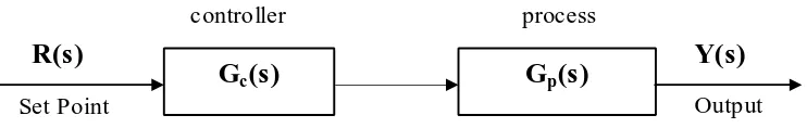
An open-loop control system is controlled directly, and only, by an input signal, without the benefit of feedback. Open-loop control systems are not as commonly used as closed-loop control systems because of the issue of accuracy. We shall therefore develop its technique of control, and further extend the knowledge gathered to more advanced control loops the have the potential to attain accuracy. An open loop structure is shown in figure 1 below.
Figure 1 : Open loop control scheme
With the controller Gc(s), set to put control on the plant Gp(s), then it is clear from basic linear system theory that the output Y(s) can be modelled as the product of the linear blocks as follows:
Y(s) = R(s)G
c(s)G
p(s)
If we assume there exists a model of the plant with a transfer function modelled as Gpm(s) such that Gpm(s) is an exact representation of the process (plant), i.e.
Gpm(s)= Gp(s), then set point tracking can be achieved by designing a controller such that:
G
c(s) = G
pm(s)
-1This control performance characteristic is achieved without feedback and highlights two important characteristic features of this control modelling [3]. These features are as follows:
perfect control can be theoretically achieved if complete characteristic features of the process are known or easily identifiable.
feedback control is only necessary if knowledge about the process is inaccurate or incomplete.
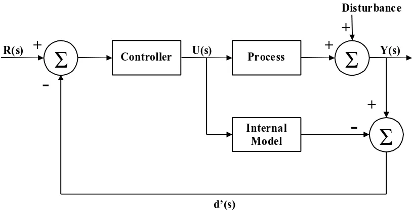
This control performance as already said has been achieved without feedback and assumed that the process model represent the process exactly i.e. the process model has all features of the parent process. In real life applications, however, process models have capabilities of mismatch with the parent process; hence feedback control schemes are designed to counteract the effects of this mismatching. A control scheme that has gained high popularity in process control has been formulated and known as the Internal Model Control (IMC) scheme. This design is a simple build up from the ideas implemented in the open loop control strategy and has a general structure as depicted by Figure 2 below:
G
c(s)
G
p(s)
Output Set Point
Y(s)
R(s)
[image:15.612.131.502.223.282.2]Figure 2
: Internal model control scheme
From the figure above we shall use the following conventions to describe the blocks in the system:
controller - Gc(s)
process - Gp(s)
internal model - Gp m(s)
disturbance – d(s)
disturbance transfer function – D(s)
The figure above shows the standard linear IMC scheme where the process model Gpm(s) plays an explicit role in the control structure. This structure has some advantages over convectional feedback loop structures. For the nominal case Gp(s) =Gpm(s), for instance, the feedback is only affected by the disturbance D(s) such that the system is effectively open loop and hence no stability problems can arise. This control structure also depicts that if the process Gp(s) is stable, which is true for most industrial processes, the closed loop will be stable for any stable controller Gc(s). Thus, the controller Gc(s) can simply be designed as a feedforward controller in the IMC scheme.
From the IMC scheme depicted in Figure 2 above, the feedback signal is represented as follows:
d’(s) =[ Gp(s) -Gpm(s)]U(s)+D(s) Equation 2.1
As said above, if the model is an exact representation of the process then d’(s) is
simply a measure of the disturbance. If there exist no disturbance, then d’(s) is simply a measure in difference in behaviour between the process and its model.
The closed loop transfer function of the IMC scheme can be seen modelled as below:
Σ
ProcessInternal
Model
Σ
Disturbance
R(s)
+
-
-
+
+
+
+
U(s)
+
Controller
d’(s)
Y(s)
+
(s)
c
(s)]G
pm
G
(s)
p
[G
1
(s)]D(s)
pm
(s)G
c
G
[1
(s)
p
(s)G
c
R(s)G
Y(s)
Equation 2.2The above transfer function will be shown to exist in the next section on transfer functions. From this closed loop analysis, we can see that if we design a controller such that Gc(s) =Gpm(s)-1 where the process model is an exact representation of the process, then the design will y ield good set point tracking and disturbance rejection. The controller is then detuned for robustness to account for a possible plant model mismatch. This is done by augmenting the controller with a low-pass filter to reduce the loop gain for high frequencies [3]. This idea also counteracts the effects of model inversion, as the pure inverse of the model is not physically realizable. The inversion of the process model may also lead to unstable controllers in case of unstable zeros in the model.
2.3 Internal Model Control Properties
In the IMC scheme shown by figure 2 above, the Internal Model loop calculates the difference between the outputs of the process and that of the Internal Model. This difference simply represents the effects of the disturbances and uncertainties as well as that of a mismatch of the model. Internal Model control devices have shown to have good robustness properties against disturbances and model mismatch in the case of the linear model of the process.
A control system is generally required to regulate the controlled variables to reference commands without steady state error against unknown and unmeasurable disturbance inputs. Control systems with this nature property are called servomechanisms or servo systems. In servomechanism system design, the internal model control principle plays an important role. Hence the design of a robust servomechanism system with plant uncertainty begins with three specifications as outline below:
definition of the plant model and associated uncertainty
specification of inputs
desired closed loop performance
IMC theory provides a systematic approach in the synthesis of a robust controller for systems with specified uncertainties. This brings about the two important advantages of applying IMC control scheme in the synthesis of a servo controller.
1. the closed-loop stability can be assured by choosing a stable IMC controller 2. the closed-loop performances are related directly to the controller parameters,
which makes on-line tuning of the IMC controller very convenient.
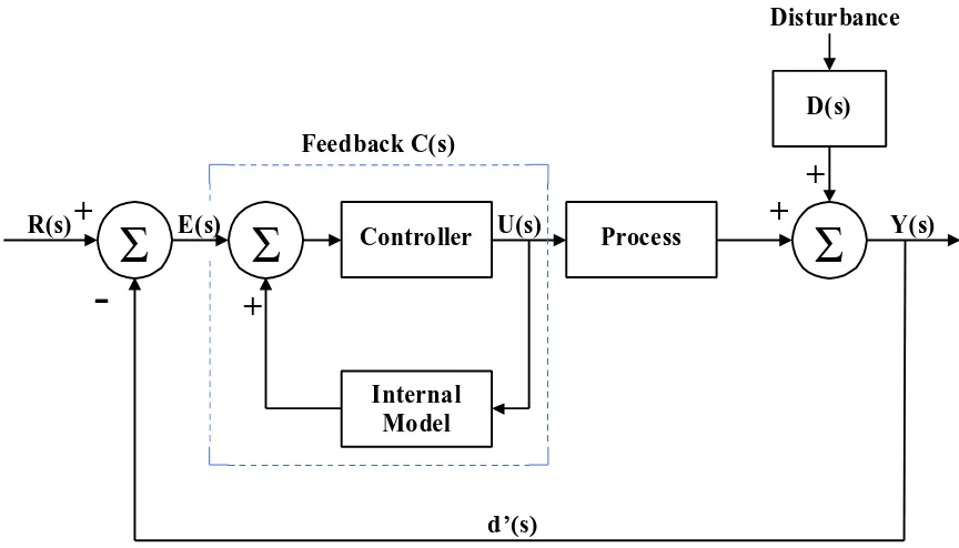
2.3.1 Transfer Functions
Figure 3: Alternate design of IMC scheme
From linear system theory in block reduction techniques, it has been shown that the transfer function between any input and the output of a single loop feedback system is the forward path transmission from the input to the output divided by one plus the loop transmission for negative feedback. Then we can establish the following equations:
)
(
)
(
1
)
(
)
(
)
(
)
(
s
pm
G
s
c
G
s
c
G
s
E
s
U
s
C
Equation 2.3Therefore the input-output relationship of figure 3 is given by the following mathematical equations:
)
(
)
(
1
)
(
)
(
)
(
)
(
s
C
s
p
G
s
C
s
p
G
s
R
s
Y
Equation 2.4)
(
)
(
1
)
(
)
(
)
(
s
C
s
p
G
s
D
s
d
s
Y
Equation 2.5Internal Model Disturbance R(s)
+
-
+
+
+
+
U(s)+
Controller Y(s)
)
(
)
(
)
(
)
(
)
(
1
)
(
)
(
)
(
1s
G
s
R
s
Y
s
C
s
p
G
s
C
s
R
s
U
p
Equation 2.6Equation 2.7
Substituting equation 2.3 into equation 2.4 and 2.5 the overall result comes to be shown as below:
)
(
)
(
)
(
1
)
(
)
(
)
(
)
(
s
c
G
s
pm
G
s
p
G
s
R
s
c
G
s
p
G
s
Y
Equation 2.8aOR
)
(
)
(
)
(
1
)
(
)
(
)
(
1
)
(
)
(
)
(
)
(
s
c
G
s
pm
G
s
p
G
s
D
s
G
s
G
s
G
s
G
s
R
s
Y
c p pm c
Equation 2.8b
2.3.2 No Offset Property of IMC
The steady state gain of any stable transfer function can be obtained by replacing the Laplace variable s with zero. If equations 2.8a and 2.8b are stable and if we choose the steady state gain of the controller Gc(0) to be the inverse of the process model gain such that Gc(0)Gpm(0)= 1, then the gain on the denominators of equation 2.8a and
equation 2.8b is effectively Gc(0)Gp(0). Therefore the gain between the set point R(s)
and Y(s) is essentially equal to one and hence the gain between the disturbance d(s) and the output Y(s) is zero. These results prove that there is no steady state deviation of the process output from the setpoint.
2.3.3 Perfect Control
If we assume that the controller is equal to the model inverse, and that the closed loop system in figure 2 is stable, then Y(s)=R(s) for all disturbances affecting the system.
2.4 Designing for IMC
The design procedure for Internal Model Control comprises two major steps. In the first step, the IMC controller is designed to achieve so-called nominal performance
without regard to plant uncertainty or equivalently with the assumption that the process model is an exact representation of the process i.e. Gpm(s) =Gp(s).in the second step, the IMC controller is augmented with a robustness compensator Gf(s) to meet the robustness specifications. This robustness compensator is usually a low pass filter of appropriate order as it is meant to counteract the increase in frequency of the plant uncertainties as well as the unmodelled dynamics of the overall system. Thus the IMC controller has the form below:
Equation 2.9
where Gc(s) is an optimal controller obtained in the first step. If the reference nominal model, the IMC controller, and the robustness compensator (low-pass filter) are appropriately designed, the IMC control scheme will produce a servo controller with desired robustness performances.
2.4.1 Practical Design of IMC
The design procedure for designing an IMC controller involves two basic steps. The steps are summarised below;
Step 1: Given the transfer function of the process model, it is required that the transfer of the model be factorised into invertible and non-invertible components
where we shall use the following conventions to relate to the relevant terms:
Gpm s invertiblecomponents
( )
Gpm s noninvertiblecomponents
( )
With this transition, it implies that with steps one, we only need to show the model in the following representation if the process to be controlled contains both the invertible and non-invertible components:
Equation 2.10
Step 2: With the transition from step one, the designer’s task is to select or model the controller as the inverse of the invertible components i.e. it is required that the controller be given the following representation:
Equation 2.11
If the process model contains only components which cannot be factorised but is does show stability with no right half poles (RHP) on the s-plane then the model is
considered invertible and the controller takes the form shown by equation 2.11. If the process model contains only the non-invertible components and with instability, then
) ( ) ( )
(s Gpm s Gpm s
pm
G
1
)
(
)
(
s
pm
G
s
c
G
)
(
)
(
)
(
s
f
G
s
c
G
s
IMC
stability and the invertibility of the process model. The non-invertibility of components may lead instability and realisability problems when inverted.
2.4.2 IMC Filter Design
The principal objective in the utilization of the IMC scheme into controlling a plant or process is to design an IMC controller GIMC(s) which comprise an optimal controller augmented with a low pass filter as shown in the figure below:
Figure 4: IMC Scheme with a Filter
The transfer function of the filter shall be represented in this document as Gf(s), with the filter in cascade with the controller. Hence, we have the IMC controller as formulated below:
)
(
)
(
)
(
s
G
f
s
G
c
s
IMC
G
Equation 2.12The filter is modelled as below:
Equation 2.13
where f is the filter parameter and n is the order of the filter.
The order of the filter is chosen such that GIMC(s) is proper to prevent excessive differential control action. In this case the order of the filter is chosen as being the
Σ
Internal
Model
Σ
Disturbance
R(s)
+
-
-
+
+
+
+
U(s) Controller
d’(s)
Y(s)
+
Σ
Process Filter
n
s)
f
τ
(1
1
(s)
f
G
same as the order of the process as will be shown in the next chapter on process modelling and IMC design.
2.5 IMC Applications
There are a lot many areas where the principle of IMC can be utilised. In essence the use of control is extremely broad and it encompasses a number of different
applications, thus this include control of electromechanical systems, where computer controlled actuators and sensors regulate the behaviour of the system, control of electronic systems, where feedback is used to compensate for component variation and provide reliable, repeatable performance and control of information and decision systems where limited resources are dynamically allocated based on estimates for future needs.
In recent year more advancements in control systems has led to more technical and reliable control schemes such as the Internal Model Control. IMC control technology has spread far beyond its initial applications. Visible success from the past
investments in IMC control includes the following:
Control systems in the manufacturing industries, from automotive to integrated circuits. Computer controlled machines provide the precise positioning and assembly required for high quality, high yield fabrication of components and products.
Industrial process control systems, particularly in the hydrocarbon and chemical processing industries. These maintain high product quality by
monitoring thousands of sensor signals and making corresponding adjustments to hundreds of valves, heaters, pumps, and other actuators.
Guidance and control systems for aerospace vehicles, including commercial aircraft, guided missiles, advanced fighter aircraft, launch vehicles, and satellites. These control systems provide stability and tracking in the presence of large environmental and system uncertainties.
Control of communications systems, including the telephone system, cell phones, and the Internet. Control systems regulate the signal power levels in transmitters and repeaters, manage packet buffers in network routing
equipment, and provide adaptive noise cancellation to respond to varying transmission line characteristics.
These applications have had an enormous impact on the productivity of modern society. In addition to its impact on engineering applications, IMC control has also made significant intellectual contributions. Control theorists and engineers have made rigorous use of and contributions to mathematics, motivated by the need to develop provably correct techniques for design of feedback systems. They have been consistent advocates of the “systems perspective,” and have developed reliable systems perspective,” and have developed reliable perspective,” and have developed reliable have developed reliable developed reliable reliable
3.0 Chapter Three: Servo System and Modelling
This section of the project is looking primarily into introducing how the plant is modelled as an extension for collaborative use in the discussion of the simulation in internal model control (IMC) and PID implementations for this project. The section discusses two features of the project as listed below.
P lant Modelling in mathematical terms
Servo System controllers (IMC and PID)
3.1 Servo Background
Servo control, which is also referred to as "motion control" or "robotics" is used in industrial processes to move a specific load in a controlled fashion. These systems can use either pneumatic, hydraulic, or electromechanical actuation technology. The choice of the actuator type (i.e. the device that provides the energy to move the load) is based on power, speed, precision, and cost requirements. Electromechanical systems are typically used in high precision, low to medium power, and high-speed applications. These systems are flexible, efficient, and cost-effective. Motors are the actuators used in electromechanical systems. Through the interaction of
electromagnetic fields, they generate power. These motors provide either rotary or linear motion.
Servo drives and amplifiers are used extensively in motion control systems where precise control of position and/or velocity is required. The drive/amplifier simply translates the low-energy reference signals from the controller into high-energy signals to provide motor voltage and current. In some cases the use of a digital drive replaces the controller/drive or controller/amplifier control system. The reference signals represent either a motor torque or a velocity command and can be either analogue or digital in nature.
3.1.1 Overview
The extension of modelling the plant for this project emanates from a build up of electric motors which are almost universally used in modern commercial and industrial occupancies to furnish the required mechanical motive power to drive mechanical machinery and control various industrial processes. Such machinery or other mechanical devices (valves, mechanical linkages, etc) connected to motor shafts (either directly or coupled through gears, belts or pulleys) are called motor loads or in simpler terms just loads. In many cases, a load must be driven at a variety of speeds in either direction, in accordance with some desired preset sequence (for example; an elevator in a high rise building). Frequently, several motors are required in
combinations in more complex sequences to control interrelated loads (as happens in chemical plants and still mills).
utilized in Internal Model Control theory come into play from this point of view to design a controller used in this context. A controller may be manually operated by maybe an experienced human operator or can be made to run in an automated fashion. The degree of automation is dictated by the requirements of the process to be
controlled. Where more precise control of the process or load speed and torque is indicated, closed loop control is utilized, and the controller and its associated control devices are somewhat more complex and complicated. In part, the selection of the type of motor used is dictated by the nature of the load requirements, the type of energy available and the types of controller commercially manufactured to adequately meet the load requirements.
3.1.2 Mathematical Model
The goal in the development of the mathematical model is to understand in mathematical terms the behaviour of the system without control before we can put control over it. Therefore, modelling simple servo systems can be developed by considering the electrical and mechanical characteristics of the system. In this context we shall consider a simple servo-DC position control servomechanism.
The basic form of a DC servo system is made of an electric motor with an output shaft that has an inertial load J on it, and friction in the bearings of the motor and load. There exist an electric drive circuit where an input voltage u(t) is transformed into a torque T(t) in the motor output shaft. The general view of this interpretation is shown by the schematic below:
Using system-modelling ideas for mechanical systems a torque balance can be written between the input torque from the motor and the torque
required to accelerate the load and overcome friction. This can be modelled by
the following equation from Newton’s second law of motion, F=ma:
Equation 3.1
)
(
.
..
t
T
b
J
A
u(t)
I
aJ
ώ
aElectrical
part
Where
is the angular position of the servo output shaft; and b is a constant representing the friction in the bearings of the motor and the load. The principle involved in the control objective is simp ly to control the angular position
or the shaft velocity to be some desired value. The input voltageu(t)
is related to the torqueT(t)
by a gain K. The system model reduces to the following:)
(
.
..
t
Ku
Equation 3.2where
is the system time constant defined by J/b while K is the system gain defined by 1/b.In practical servomechanisms there are additional components of the system which are obviously important. Many of these will relate to nonlinearities in the drive amplifier and friction in the mechanical components of the system, hence a good control system must incorporate these features to overcome the nonlinear characteristics.
In this section and for the project we concentrate our modelling on the linear parts of the servo system for simplicity. The linear part of the servo system model for this project can be put in transfer function form as follows:
u(s)
6)
s(
τ(
K
y(s)
Equation 3.3where
y(s)
is the system output andu(s)
is the system input. The parameters for the project are therefore defined as: (i) system gain K = 109(ii) system time constant = 1 (iii) inertial load J = 1/109 (iv) friction constant b = 1/109
With the growing interest on high performance of a mechanical positioning system, more accurate and robust control algorithms are required. The control technique set in
this document is looking into providing control to a servo system modelled as below:
Equation 3.4
The aim of the project is now to utilize the techniques of IMC and PID algorithms to provide control to the process modelled above. This idea will of the design will follow in the next chapter, first we shall establish the principles of PID implementations and design in the next chapter and follow with the techniques associated with the design for Internal Model Control.
6)
s(s
109
(s)
p
G
3.2 Servo System Controllers
There are many alternative control design theories that can be used to control a servomechanism. In this project we are looking into using two of the many forms and document analysis on their control performance with respect to the modelled
servomechanism above. These two control mechanism include the convectional PID used widely in commercial and industrial applications and secondly we look into a model based approach in Internal Model Control (IMC) to see what sort of control results we achieve with these two control schemes on their control performance actions when providing control to a servo system.
While Internal Model Control implementations are becoming more popular, the standard industrial controllers remain the proportional (P), proportional plus integral (PI), and the proportional plus integral and derivative (PID) controllers. Morari and Zafiriou (1989) and Rivera et al. (1986) show how to approximate the IMC controller for a limited class of processes with PI and PID controllers. To obtain a PID controller for the industrially important first-order lag and dead time process model, they
approximate the dead time with a low-order Padé approximation. Because their approximations are surprisingly good enough, they conclude that there is relatively little to be gained in dynamic response by implementing the IMC controller rather than the PI or PID approximations.
The controller is the "brains" of a servo system. It is responsible for generating the motion paths and for reacting to changes in the outside environment. Controllers can be something as simple as an ON/OFF switch or a dial controlled by an operator. They can also be as complex as a multi-axis controller that actively servos several drives as well as monitors I/O and maintains all of the programming for the machine.
4.0 Chapter Four: PID Control for the Servo System
4.1 Introduction to PID controllers
Proportional-Integral-Derivative controllers are the most common controllers in electric drives and many other applications of the process industry. PID control is widely used in servo systems as it has a simple structure, safety and reliability. In the superposition design approach PID control can be viewed as combining proportional, derivative and integrating elements or some system signal weighted by a factor. The popularity of these controllers has led to research on tuning methods resulting in numerous methods published over the years. The most popular and acceptable methods relate to work done in recent publications by Ziegler-Nichols.
However, the tuning of the PID control systems is not always easy, because of its simple control structure for wide class of process characteristics. The PID controller has three tuning parameters which can be tuned by trial and error or by using tuning rules available in literature such as the Ziegler-Nichols. These rules are based on the open-loop stable first order or second order plus dead time process models or critical point information for stable processes. However, under certain circumstances published tuning rules or methods may not provide satisfactory closed loop
performances. This document is looking forward to extend the knowledge that may have already been existence by exploring the principles involved in PID parameter representation as well as tuning techniques.
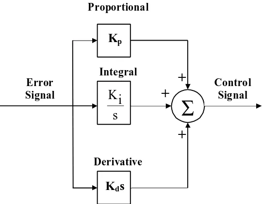
[image:27.612.120.390.444.655.2]4.2 PID Mathematical representation
Figure 4.1: Proportional-Integral-Derivative (PID) controller
Figure 4.1 above shows how the PID parameters are represented in a control architecture. Whatever the nature of the process, there will be some desired point of
Σ
Error Signal
Control Signal
K
pProportional
Integral
s
i
K
Derivative
K
ds
operation, and some difference from that desired point, usually called the error. The technique in control is to minimize such an error to a value as close to zero as possible. By employing feedback to a control scheme we desire to replicate the error to a control command so that we conceive appropriate control action for better performance of the overall system. The PID achieves this principle with its parameters as it imposes the following commands to an incoming error:
1. it ensures that its response has a related proportion to the magnitude of the error
2. it has the ability to take stronger action should the error persist in time 3. it has the ability to act quickly at the onset of error in an attempt to get ahead
of it
The time domain representation of the PID control output is given as PID(t) below:
t
dt
t
de
D
T
dt
t
e
i
T
t
e
c
K
t
PID
0
)
(
)
(
1
)
(
)
(
Equation 4.1where the following conventions apply:
Kc– controller gain
e(t) – error signal
Ti - integral time
TD– derivative time
4.3 PID Parameter Characterisation
This section is set to define the action attributes of each of the PID parameters, the proportional, the integral and the derivative.
4.3.1 Proportional Command
Figure 4.2: Proportional Control
The figure above shows the proportional control. The proportional control imp lies that if you have a reference you are trying to control to, you simply provide a control output proportional to the error from your reference. Hence from the above we shall
set
point
measured
value
+
K
pΣ
-
e(t)
control
Control effort = K
p* (Set Point
–
Measured Value)
Equation 4.2where the error
e(t) = Set Point
–
Measured Value
4.3.2 Integral CommandFigure 4.3: Integral Control
Figure 4.3 above shows the integral control action. The integral is needed mainly for the off-sets and biases in the system. The integral term yields zero steady-state error in tracking a constant set point. Integral control enables also enables the complete rejection of constant disturbances. While integral control filters higher frequency sensor noise, it is slow in response to the current error.
The integral exists in the system to calculate the integral of the input over time. It uses the input to create an output which will continue to grow until the input is reduced to zero. Thus the control effort is summarised below:
Control effort = K
i* (Integrator Output)
Equation 4.34.3.3 Derivative Command
Figure 4.4: Derivative Control
Figure 4.4 shows the derivative control action from the PID algorithm. For process with significant dead time, the effects of the proportional and the integral actions are poorly represented in the current error. This situation may lead to large transient
set
point
measured
value
+
K
i-
e(t)
control
effort
integrator
Σ
set
point
Measured value
+
K
i-
e(t)
control
effort
rate taker
dt
d
errors when PI control is used. The derivative control action combats this problem by basing a portion of the control on a prediction of the future error. Unfortunately, the derivative amplifies higher frequency sensor noise; thus, a filtering of the
differentiated signal is typically employed, introducing an additional tuning parameter.
The derivative tells how fast a signal is approaching or departing from a set point. The important signal in the above configuration is the rate signal that is output of the rate taker and multiplied by the derivative constant to provide the control effort. Hence
Control effort = K
d* Rate
Equation 4.4The overall control effort becomes the sum of the efforts to represent the standard PID algorithm. We therefore represent the overall control effort as
u(t)
as follows:
dt
t
de
d
K
dt
t
e
i
K
t
e
p
K
t
u
(
)
(
)
(
)
(
)
Equation 4.54.4 PID Design for the Servo System
There are typical steps chosen as rule of thumb to design a PID controller. The following steps works in many cases:
1. determine what characteristics of the system need to be improved. 2. use the proportional gain Kpto reduce the rise time.
3. use the derivative gain Kd to reduce the overshoot and settling time 4. use the integral gain Ki to eliminate the steady state error
There are design methods though that has been put into literature which simplifies the need for beating about the bush. We shall explore one of these ideas here and utilise in the design of our PID for the servo system. This method is famously known as the Ziegler-Nichols method and is chosen in this context because it is simple and a little straight forward.
Figure 4.5: An S-shaped open loop response of a system
Controller Proportional Kp
Integral Ki
Derivative Kd
PID
L T
5 .
0 0.6 2
L
T 0.6T
Table 4.1
It is estimated that with these parameters set as above, a response with an overshoot of 25% and good settling time should be obtained. Fine tuning will then be necessary if the performance deviates from optimal. This can be done using the basic rules that relate each parameter to the response characteristics.
However, in the ZN method, tuning is based on the critical gain and the period, which are determined by increasing the proportional gain until the stability limit is reached. In practice, this method may cause the risk of instability and it is difficult to automate, but forms a development of a tuning mechanism that has the potential to achieve optimal control.The ZN tuning rule uses the ultimate information of the process. Therefore, it cannot systematically consider the concrete control performance to tune the PID parameters.
From the open loop response we approximate the values of the two parameters L and T as derived from figure 4.6 below:
L= 1.2
[image:31.612.126.538.84.294.2]These values are then used as per table 4.1 to calculate the settings of the PID parameters which can be deduced from table 4.2. Using this values the PID
parameters are set as direct in simulink to produce a plot of a response to a step input. These implementations and results can be seen in the section that follows.
See: Model M4.1 below: Simulink Implementations
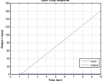
In the above model, an open loop response was to be observed. A step input as reference was applied to the plant without a controller. It was therefore important to link the matlab workspace with the simulink environment by linking the two
environments with the simout block. In this way the matlab can reference all outputs from simulink to some memory address, and thus can be used further in the
simulations.
The response curve in open loop is shown in figure 4.6 below. With all concepts of the ZN tuning method put in mind, the response curve can be used to verify the parameters as shown by figure 4.5. These parameters can then be further explored to evaluate the PID parameters as per table 4.1.
Hence the values of the PID controller can be set as below in Table 4.2. (ZN First Trail), with the help of the values obtained from figure 4.6 below. i.e.
L= 1.2
T= 9.8
u inp ut
109 s +6s2
Se rvo t Time
Step Sc ope
y Outp ut Clock
0 1 2 3 4 5 6 7 8 9 10 0
20 40 60 80 100 120 140 160 180
Open Loop Response
O
u
tp
u
t
v
I
n
p
u
t
Time (se c)
[image:33.612.127.471.79.350.2]input output
Figure 4.6: Open Loop response to a step Input for Ziegler-Nichols First Trial
Table 4.2
Controller Proportional Kp
Integral Ki
Derivative Kd
PID 4.083 3.7 5.88
See: Model M4.2:
y o utput u
input
t Tim e Step Inp ut
109 s +6s2 Se rvo S ys te m
Scope PID
PID Co ntroller
C lock
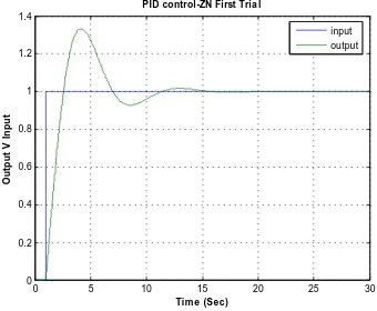
On simulation of the above system having set the parameters of the PID as per table 4.2 we get the response as shown on figure 4.7 below.
0 5 10 15 20 25 30
0 0.2 0.4 0.6 0.8 1 1.2 1.4
PID control-ZN First Tria l
Tim e (Sec)
O
u
tp
u
t
V
I
n
p
u
t
[image:34.612.130.470.101.381.2]input output
Figure 4.7: PID control-ZN first Trial
With the first trial on application of the Ziegler-Nichols PID parameter setting, it is evident that the response is offset in set point tracking with an overshoot and the next trial involves fine tuning the parameters to get the best response. This can be done with the help of the following Table 4.3 which shows the effects of increasing each of the PID parameters on the response characteristics.
Response Rise Time
Overshoot Settling Time Steady-State ErrorKp Decrease Increase Inconclusive Decrease
Ki Decrease Increase Increase Eliminates
Kd Inconclusive Decrease Decrease Inconclusive
Table 4.3
Based on Model M4.2 from Appendix, PID parameters were tuned by trial and error to obtain the best response with the following settings on the second trial:
Table 4.2
Controller Proportional Kp
Integral Ki
Derivative Kd
Using these new values after a tremendous effort of refining the response, the new version of the response is observed as per figure 4.8 below. There is little overshoot in the response and setpoint tracking can be easily achieved. The response is shown below:
0 1 2 3 4 5 6 7 8 9 10
0 0.2 0.4 0.6 0.8 1 1.2 1.4
P ID control-ZN Second Trial
O
u
tp
u
t
v
I
n
p
u
t
Time (se c)
Figure 4.8: PID control-ZN Second Trail
4.5 Disturbance effects with PID design
In this section we are looking into establishing the effects of disturbances at both the input and the output of the plant with the best PID parameters as per table 4.2. For simplicity we shall model disturbances as a simple step input and a sinusoidal wave and see how the response deviates from the optimal response.
4.5.1 Step Input Disturbance at the input of the Plant
The output plots for the above simulation in simulink can be seen below in figure 4.9.
0 1 2 3 4 5 6 7 8 9 10
0 0.2 0.4 0.6 0.8 1 1.2 1.4
PID control+Ste p Disturbance Input
O
u
tp
u
t
v
I
n
p
u
t
Time (se c)
input output
Figure 4.9: PID control under a step disturbance at input of plant
It can be seen from the output results that if a step disturbance is introduced at the input of the plant, the response deviates form the optimal response with a little offset of an overshoot but then sets a little later to follow the set point.
y o utput u
input t
Time
Step Input1 Step Input
109 s +6 s2 Servo S ystem
Scope PID
P ID C ontroller Cloc k
4.5.2 Sinusoidal Disturbance at the input of the plant
Simulink Implementations: See below
y output u
input t
T im e
Step Input
Si ne Wave
109 s +6s2 Servo System
Scope PID
PID Controll er Clock
On simulation of the above system with a sinusoidal disturbance at the input of the plant, the response to a step input can be shown as in figure 4.10 below.
0 1 2 3 4 5 6 7 8 9 10
0 0.2 0.4 0.6 0.8 1 1.2 1.4
PID control+Sinusoida l Disturba nce Input
O
u
tp
u
t
v
I
n
p
u
t
Time (se c)
input output
Figure 4.10: PID control under a Sinusoidal disturbance at input of plant
It can be seen here that with a sinusoidal disturbance at the input of the plant, control action is lost and the response becomes oscillatory around the setpoint. This shows
poor performance as far as manipulation of the error signal is concerned. Further tuning of the PID parameters by trial and error is therefore necessary to attain the optimal response.
4.5.3 Step Input Disturbance at the output of the Plant Simulink Implementations: See below
On simulation of the above system the response is plotted as per figure 4.11 below:
0 1 2 3 4 5 6 7 8 9 10
0 0.1 0.2 0.3 0.4 0.5 0.6 0.7 0.8 0.9 1
PID control+Ste p Disturba nce (Plant Output)
O
u
tp
u
t
v
I
n
p
u
t
Time (se c)
input output
Figure 4.11: PID control with step input disturbance at output of plant
y output u
inp ut t
Time
Step Input1 S tep Inp ut
109 s +6s2 Servo S ys te m
Sc ope P ID
PID Co ntro ller C lock
With a step input at the output of the plant, set point tracking and disturbance rejection is achieved as can be seen from the output of the scope and as per figure 4.11 above. The output is perfectly embedded on setpoint, hence perfect setpoint tracking and disturbance rejection.
4.5.4 Sinusoidal Disturbance at the output of the Plant
Simulink Implementations: See below:
0 1 2 3 4 5 6 7 8 9 10
0 0.2 0.4 0.6 0.8 1 1.2 1.4
PID control+Sinusoidal Disturbance (Pla nt Output)
O
u
tp
u
t
v
I
n
p
u
t
Time (se c)
input output
Figure 4.12: PID control with a sinusoidal disturbance at the output of plant
y outp ut u
inp ut t
Time
Step Input
S ine Wa ve 109 s +6s2 Se rvo S yste m
Sc ope P ID
PID Contro lle r Clock
On simulation of the above system (Model M4.6) the response is as in figure 4.12 above. The response cannot be seen as oscillatory anymore and it simulates that of a step disturbance at the input of the plant.
It can also be seen that the offset from set point tracking is not too big as was seen with the sinusoidal disturbance at the output of the plant. Perfect control is
theoretically possible in this instance as there is a little overshoot in the response of which settles quickly to attain setpoint tracking.
0 1 2 3 4 5 6 7 8 9 10
0 0.2 0.4 0.6 0.8 1 1.2 1.4
Tim e (Sec)
O
u
tp
u
t
V
s
I
n
p
u
t
Step Disturba nce a t both Output & Input of Pla nt
reference output
Figure 4.13: PID Control (Step Disturbance at both Input and Output)
t T ime
Step(Reference)
Step(Disturbance)1 Step(Disturbance)
109 s +6s2 Servo
Scope PID
PID Controller
y Output u Input Clock
It was interesting to observe the output as the process is made subject to a step
disturbance at both the input and output as shown by model M4.7. The response curve as shown in figure 4.13 shows the output. The response curve overshoots and settles to setpoint at a period of about seven seconds. Not a bad setpoint tracking though! Tuning the parameters may be needed to adjust tracking time to minimal.
0 1 2 3 4 5 6 7 8 9 10
0 0.2 0.4 0.6 0.8 1 1.2 1.4
Tim e (Sec)
O
u
tp
u
t
V
s
I
n
p
u
t
PID control (Sinusoida l Disturba nce at both Input and Output)
reference output
Figure 4.14: PID Control (Sinusoidal Disturbance at both Input and Output)
Model M4.8: Sinusoidal Disturbance at both output & input of
Plant
t T ime
Step(Reference)
Sine Wave (Disturbance)1 Sine Wave (Disturbance)
109 s +6s2 Servo
Scope PID
PID Controller
Model M4.8 shows a system where a process is subject to a sinusoidal disturbance at both the input and output. In practice such disturbances are difficult to put under control because they add new dynamics to the system. The response curve to the model above is shown in figure 4.14. The response is oscillatory which shows poor performance as far as the PID control effort is concerned. Good regulatory behaviour will be attained by proper tuning of the gains.
4.6 SIMULINK Implementations
All SIMULINK implementations are as shown in each section described above. Relative discussion is also taken briefly in each step of the system simulations.
4.7 Results and Analysis
5.0 Chapter Five: IMC design for the Servo System
5.1 IMC Controller
The principal objective in the utilization of the IMC scheme into controlling Gp(s) is to design an IMC controller GIMC(s) which comprise a series combination of Gc(s) and Gf(s) where Gf(s) is a low pass filter of appropriate order. Hence:
G
IMC(s) = G
f(s)G
c(s)
Equation 5.1Therefore, from the steps in designing the controller, we already established that the controller will replicate the inverse of the process model as per the Equation below:
G
c(s) = G
pm(s)
-1Equation 5.2
If we assume the process model exactly matches the parent process, then the principle in designing the controller Gc(s) is to set Gc(s) as below:
Equation 5.3
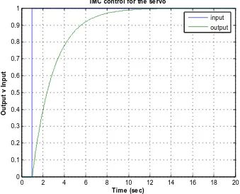
5.2 Filter Design for the Servo System
In Internal Model Control a filter is normally augmented with the optimal controller to attenuate the effects of process-model mismatching and remove the higher frequency part of the noise in the system in order to meet robust specifications. The robust compensator (filter) plays a pivotal role in the system as it combats plant uncertainties in the system design so that the designed control system can achieve the design objectives of robust stability and robust performance.
The filter is modelled as below from basic control system theory :
Equation 5.4
where
f is the filter parameter and n is the order of the filter. The order of the filter ischosen such that GIMC(s) is proper to prevent excessive differential control action. The filter parameter in the design can be chosen as a rule of thumb; hence the filter parameter values are often dictated by modelling errors, as has already stated that in the design, it remains the only tuneable parameter. In this application we would like to simulate the system with n=2 to make GIMC(s) proper. We would also like to tune the
n
s)
f
τ
(1
1
(s)
f
G
109
6s
2
s
(s)
c
filter parameter such that it is to be at least twice as fast as the open loop response. Therefore the filter of interest is now modelled as below with n=2;
Equation 5.5
The filter parameter
f remains the only tuneable parameter. Therefore the IMCcontroller becomes a cascade combination of the optimal controller Gc(s) and