Diesel engine performance and exhaust emission analysis using waste cooking biodiesel fuel with an artificial neural network

Diesel engine performance and exhaust emission analysis using waste

cooking biodiesel fuel with an artificial neural network

B. Ghobadian a, H. Rahimi a, A. M. Nikbakht a, G. Najafi a and T F Yusaf b

a

Tarbiat Modares University, Tehran - Iran P.O.Box:14115-111

b

University of Southern Queensland, Toowoomba, 4350 QLD, Australia

Abstract

This study deals with artificial neural network (ANN) modeling a diesel engine using waste cooking biodiesel fuel to predict the brake power, torque, specific fuel consumption and exhaust emissions of engine. To acquire data for training and testing the proposed ANN, two cylinders, four-stroke diesel engine was fuelled with waste vegetable cooking biodiesel and diesel fuel blends and operated at different engine speeds. The properties of biodiesel produced from waste vegetable oil was measured based on ASTM standards. The experimental results reveal that blends of waste vegetable oil methyl ester with diesel fuel provide better engine performance and improved emission characteristics. Using some of the experimental data for training, an ANN model based on standard Back-Propagation algorithm for the engine was developed. Multi layer perception network (MLP) was used for nonlinear mapping between the input and the output parameters. Different activation functions and several rules were used to assess the percentage error between the desired and the predicted values. It was observed that the ANN model can predict the engine performance and exhaust emissions quite well with correlation coefficient (R) were 0.9487, 0.999, 0.929 and 0.999 for the engine torque, SFC, CO and HC emissions, respectively. The prediction MSE (Mean Square Error) error was between the desired outputs as measured values and the simulated values by the model was obtained as 0.0004.

Keywords: Waste cooking biodiesel, Biodiesel-diesel blends; Artificial Neural Network; Diesel engine

___________________________________________________________________________ This is the Author post-print of the following paper:

Ghobadian, Barat and Rahimi, Hadi and Nikbakht, A. M. and Najafi, Gholamhassan

and Yusaf, Talal (2009)

Energy, 34 (4). pp. 976-982. ISSN 0960-1481

1. Introduction

Rudolf Diesel invented diesel engine in 1892 and received the patent on 1893. He originally developed his engine to run on biodiesel. In 1930s and 1940s vegetable oils were used as diesel fuels, but only in emergency situations [1, 2]. Alternative fuels for diesel engines are becoming increasingly important due to diminishing petroleum reserves and the environmental consequences of exhaust gases from petroleum fuelled engines [3, 4]. A number of studies have shown that triglycerides hold promise as alternative diesel engine fuels. So, many countries are interested in that. For example, evaluation of the production of biodiesel in Europe since 1992 shows an increasing trend [5]. Waste vegetable oil methyl ester is a biodiesel. Biodiesel is defined as the mono alkyl esters of long chain fatty acids derived from renewable lipid sources. Biodiesel, as defined, is widely recognized in the alternative fuel industry. Biodiesel is typically produced through the reaction of a vegetable oil or animal fat with methanol in the presence of a catalyst to yield glycerin and methyl esters [6, 7 and 8]. The blend of 75:25 ester/diesel (B25) gave the best performance [8, 9]. Among the attractive features of biodiesel fuel are: (i) it is plant, not petroleum-derived, and as such its combustion does not increase current net atmospheric levels of CO2 a

“greenhouse” gas; (ii) it can be domestically produced, offering the possibility of reducing petroleum imports; (iii) it is biodegradable; and (iv) relative to conventional diesel fuel, its combustion products have reduced levels of particulates, carbon monoxide, and, under some conditions, nitrogen oxides. It is well established that biodiesel affords a substantial reduction in SOx emissions and considerable reductions in CO, hydrocarbons, soot, and particulate

matter (PM).

There is a slight increase in NOxemissions, which can be positively influenced by delaying

the injection timing in engines [4, 11, 12 and 33]. Artificial neural networks (ANN) are used to solve a wide variety of problems in science and engineering, particularly for some areas where the conventional modeling methods fail. A well-trained ANN can be used as a predictive model for a specific application, which is a data-processing system inspired by biological neural system. The predictive ability of an ANN results from the training on experimental data and then validation by independent data. An ANN has the ability to re-learn to improve its performance if new data are available [13].

An ANN model can accommodate multiple input variables to predict multiple output variables. It differs from conventional modeling approaches in its ability to learn about the system that can be modeled without prior knowledge of the process relationships. The prediction by a well-trained ANN is normally much faster than the conventional simulation programs or mathematical models as no lengthy iterative calculations are needed to solve differential equations using numerical methods but the selection of an appropriate neural network topology is important in terms of model accuracy and model simplicity. In addition, it is possible to add or remove input and output variables in the ANN if it is needed. The objective of this study was to develop a neural network model for predicting engine parameters like emission, fuel consumption and torque in relation to input variables such as engine speed and biofuel blends. This model is of a great importance due to its ability to predict engine performance under varying conditions.

2. Experimental investigation

2.1. Biodiesel preparation

In the present investigation, biodiesel was produced from waste vegetable oil of a restaurant. 1.8 gr KOH (as Alkali catalyst) and 33.5cc methanol (as an alcohol) was applied for 120 gr waste vegetable oil in this reaction. Biodiesel production reaction time was 1 hour with stirring and no heat. Up to one week time is needed for separation and washing process. The Waste vegetable oil methyl ester was added to diesel fuel in 10 to 50 percent ratios and then used as fuel for 2 cylinder diesel engine.

2.2. Experimental set up and test procedure

The experimental setup consists of a two cylinder diesel engine, an engine test bed and a gas analyzer. The schematic of the experimental setup is shown in (Fig. 1).

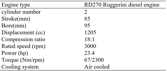
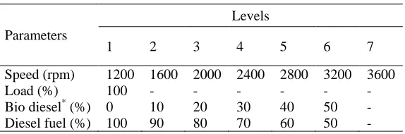
There are two fuel tanks, one is for diesel fuel and the other for fuel blends. The engine under study is a commercial DI, water cooled two cylinders, in-line, naturally aspirated, RD270 Ruggerini diesel engine whose major specifications are shown in Table 1. The test engine was coupled to a Schenck W130 electric eddy current dynamometer. A Horiba gas analyzer model MEXA-324GB was used for measuring CO and HC emissions. Engine was run at several speeds at full load and power, torque, fuel consumption and emissions was measured. The matrix of experimentation is shown in Table 2.

Fig.1. Engine test setup

Table 1

Specifications of the test engine

Engine type RD270 Ruggerini diesel engine

cylinder number 2

Stroke(mm) 85

Bore(mm) 95

Displacement (cc) 1205

Compression ratio 18:1

Rated speed (rpm) 3000

Power (hp) 23.4

Torque (Nm/rpm) 67/2300

Cooling system Air cooled

Gas Analyzer

• •

• •

Manual control

Engine Control

unit

Dynamometer

Fuel tank Alternative tank

Fuel control unit

Table 2

The matrix of experimentation

Parameters

Levels

1 2 3 4 5 6 7

Speed (rpm) 1200 1600 2000 2400 2800 3200 3600

Load (%) 100 - - - -

Bio diesel* (%) 0 10 20 30 40 50 -

Diesel fuel (%) 100 90 80 70 60 50 -

* The symbol used for Waste vegetable oil methyl ester is B

3. Neural network design

An Artificial intelligence (AI) system is widely accepted as a technology offering an alternative way to tackle complex and ill-defined problems [14]. The ANN approach has been applied to predict the performance of various thermal systems [15–23].An artificial neural network (ANN) was used for the long-term performance prediction of thermosyphonic type solar domestic water heating (SDWH) systems. Results indicated that the proposed method can successfully be used for the prediction of the solar energy output of the system for a draw-off equal to the volume of the storage tank or for the solar energy output of the system and the average quantity of the hot water per month for the two demand water temperatures considered [24]. Artificial Neural Network is a system loosely modeled on the human brain. A biological neuron is shown in (Fig. 2).

Fig. 2. A simplified model of a biological neuron

The use of ANNs for modelling the operation of internal combustion engines is a more recent progress. This approach was used to predict the performance and exhaust emissions of diesel engines [25, 26] and the specific fuel consumption and fuel air equivalence ratio of a diesel engine [27]. The effects of valve-timing in a spark ignition engine on the engine performance and fuel economy were also investigated using ANNs [28].

Basically, a biological neuron receives inputs from other sources, combines them in someway, performs generally a nonlinear operation on the result, and then outputs the final result. The network usually consists of an input layer, some hidden layers, and an output layer [29, 30]. A popular algorithm is the back-propagation algorithm, which have deferent variants. Back-propagation training algorithms gradient descent and gradient descent with momentum are often too slow for practical problems because they require small learning rates for stable learning. In addition, success in the algorithms depends on the user dependent parameters learning rate and momentum constant. Faster algorithms such as conjugate gradient, quasi-Newton, and Levenberg–Marquardt (LM) use standard numerical optimization techniques. These algorithms eliminate some of the disadvantages mentioned above. ANN

Axon Soma

Dendrit

with back-propagation algorithm learns by changing the weights, these changes are stored as knowledge. LM method is in fact an approximation of the Newton’s method [31]. The algorithm uses the second-order derivatives of the cost function so that a better convergence behavior can be obtained. In the ordinary gradient descent search, only the first order derivatives are evaluated and the parameter change information contains solely the direction along which the cost is minimized, whereas the Levenberg–Marquardt technique extracts more significant parameter change vector. Suppose that we have a function E(X) which needs to be minimized with respect to the parameter vector x [32, 34]. The error during the learning is called as root-mean squared (RMS) and defined as follows:

2 1 2 1       −       =

∑

RMS (1)

In addition, absolute fraction of variance (R2) and mean absolute percentage error (MAPE) are defined as follows respectively:

(

)

∑

∑

1 (2)

100 × − = o t o

MAPE (3)

Where t is target value, o is output value, and p is pattern. Input and output layer are normalized in the (-1,1) or (0,1) range [34]. To get the best prediction by the network, several architectures were evaluated and trained using the experimental data. The back-propagation algorithm was utilized in training of all ANN models.

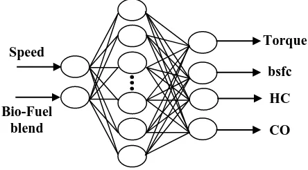
This algorithm uses the supervised training technique where the network weights and biases are initialized randomly at the beginning of the training phase. The error minimization process is achieved using a gradient descent rule. There were two input and four output parameters in the experimental tests. The two input variables are engine speed in rpm and the percentage of biodiesel blending with the conventional diesel fuel. The four outputs for evaluating engine performance are engine torque in Nm, Specific Fuel Consumption (SFC) in lit/KW.hr, and emissions including HC and CO in ppm. Therefore the input layer consisted of 2 neurons which corresponded to engine speed and levels of biofuel blends and the output layer had 4 neurons (Fig. 3).

The number of hidden layers and neurons within each layer can be designed by the complexity of the problem and data set. In this study, the number of hidden layers varied from one to two. To ensure that each input variable provides an equal contribution in the ANN, the inputs of the model were preprocessed and scaled into a common numeric range [-1,1]. The activation function for the hidden layer was selected to be logsig. Linear function suited best for the output layer. This arrangement of functions in function approximation problems or modeling is common and yields better results. However many other networks with several functions and topologies were examined. Three criteria were selected to evaluate the networks and as a result to find the optimum one among them. The training and testing performance (MSE) was chosen to be .00001 for all ANNs. The complexity and size of the network was also important, so the smaller ANNs had the priority to be selected. Finally, a regression analysis between the network response and the corresponding targets was performed to investigate the network response in more detail. Different training algorithms were also tested and finally Levenberg-Marquardt (trainlm) was selected. The computer program MATLAB 7.2, neural network toolbox was used for ANN design.

4. Results and discussion

4.1. Characteristics of biodiesel

Transesterification of the waste vegetable oil reduced the viscosity from 31.8 mm2/s to 4.15 mm2/s. This achievement paved the way to use the produced biofuel as diesel engine fuel without any engine modifications. The biodiesel high flash point makes possible its easy storage and transportation. It should be noted that the diesel fuel flashpoint is 64◦C. The biodiesel sulfur content is another interesting advantage of the produced fuel which is 18 ppm only. Comparing the 18 ppm sulfur content of the produced biodiesel with the 500 ppm sulfur content of the diesel fuel used in Tehran operating diesel vehicles, the advantage of the biodiesel over the diesel fuel in terms of the environmental benefits can be justified. This comparison indicates that the sulfur content of biodiesel produced from the waste vegetable oil in Iran is 28 times lesser than the diesel fuels used in Tehran diesel vehicles. An easy way of reducing the diesel fuel sulfur content is the biodiesel blend which is the subject matter of an ongoing research work; its result may be published in near future. Fuel properties are mentioned in Table 3.

Table 3

Properties of diesel and biodiesel fuels

Property Method Units Diesel Biodiesel

Flash point, closed cup D 93 °C 64 182

Pour point D 97 °C 0 -3

Kinematical viscosity, 40 ° C D 445 mm2/s 4.03 4.15

Sulfated ash D 874 wt. % 0.00

Total Sulfur D 5453 wt. % 0.0500 0.0018

Copper strip corrosion D 130 - 1a 1a

Cloud point D 2500 °C 2 0

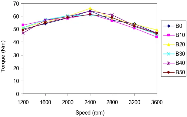
First of all, fuel rack is placed in maximum fuel injection position for full load conditions. Then, the engine is loaded slowly. The engine speed is reduced in this way with increasing load. The trend of performance curves (power and torque) are very common like those mentioned in valid concerned literature. Range of speed was selected between 1200 – 3600 rpm. Engine test results with net diesel fuel showed that maximum torque was 64.2 Nm which occurred at 2400 rpm. The maximum power was 18.12 kW at 3200 rpm. Power and torque for fuel blends at full load is shown in (Figs. 4 and 5). Considering power and torque performance with fuel blends, one can say that the trend of these parameters versus speed is perfectly similar to net diesel fuel. Fig. 4 shows engine speed and engine power relationship at full load condition using net diesel fuel and fuel blends. The net diesel fuel is used as a base for comparison. The fuel blend behavior is similar to that of net diesel fuel in developing power.

0 2 4 6 8 10 12 14 16 18 20

1200 1600 2000 2400 2800 3200 3600

Speed (rpm)

P

o

w

e

r (k

W

)

B0 B10 B20 B30 B40 B50

Fig. 4. Relationship between engine speed and engine power for different fuel blends

0 10 20 30 40 50 60 70

1200 1600 2000 2400 2800 3200 3600

Speed (rpm)

T

or

que (

N

m

)

B0

B10

B20

B30

B40

B50

Fig. 5. Relationship between engine speed and torque for different fuel blends

Fuel consumption curves of net diesel fuel at full load are shown in Fig. 6. The curves show that fuel consumption at full load condition and low speeds is high. Fuel consumption first decreases and then increases with increasing speed. The reason is that, the produced power in low speeds is low and the main part of fuel is consumed to overcome the engine friction. Irrespective of fuel consumption at low speed (1200 rpm), fuel consumption is increased with increasing speed. The reason probably is that, friction power increases with increasing speed. Fig. 6 and Table 4 show specific fuel consumption with various fuels blend percentage. The curves show that brake specific fuel consumption of fuel blends trends is very similar to net diesel fuel. Brake specific fuel consumption of fuel blends is higher than net diesel fuel. In other words, increasing fuel blend percentage, a mild increase in brake specific fuel consumption is observed.

0 0.05 0.1 0.15 0.2 0.25 0.3 0.35 0.4 0.45 0.5

1200 1600 2000 2400 2800 3200 3600

Speed (rpm)

S

F

C

(l

it

e

r/

k

W

.h

r) B0

B10

B20

B30

B40

B50

Fig. 6. Effect of fuel blends on SFC at full load and different speeds

Table 4 shows increased engine specific fuel consumption in comparison with net diesel fuel at full load condition and various speeds. This Table shows that mean value of engine specific fuel consumption of 10, 20, 30, 40 and 50% blends for various engine speeds is 4.0, 0.8, 0.6, -2.2 and 1.4 percent respectively higher than net diesel fuel.

Table 4

Variation of SFC using fuel blends with respect to diesel fuel

B0 B10 B20 B30 B40 B50

1200 0 3.6868 2.3593 1.5032 2.0153 -2.5463

1600 0 5.2771 0.9023 -3.1159 -1.6121 1.4778

2000 0 -1.9060 -0.7225 -8.5342 -14.7285 -2.1261

2400 0 4.4496 1.2458 8.2038 4.7023 7.7951

2800 0 -3.4628 -0.6258 -3.6370 -7.2545 -2.7334

3200 0 8.5685 2.2998 4.6699 1.3063 7.4125

3600 0 11.5453 0.1600 5.2294 0.0420 0.7666

4.4. Exhaust emissions

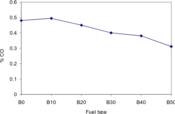
Biodiesel contains oxygen in its structure. When biodiesel is added to diesel fuel, the oxygen content of fuel blend is increased and thus less oxygen is needed for combustion. However oxygen content of fuel is main reason for better combustion and CO and HC emission reduction. Figs. 7 and 8 show the relationship between the fuel blends and CO and HC concentrations respectively.

0 0.1 0.2 0.3 0.4 0.5 0.6

B0 B10 B20 B30 B40 B50

Fuel type

% CO

Fig. 7. Effect of fuel blends on average CO emission at full load

0 5 10 15 20 25 30 35

B0 B10 B20 B30 B40 B50

Fuel type

HC (

p

p

m

)

Fig. 8. Effect of fuel blends on average HC emission at full load

4.5. Modeling with the ANN

data gathered in test runs. In the model, 80% of the data set was randomly assigned as the training set, while the remaining 20% of data are put aside for prediction and validation. A network with one hidden layer and 25 neurons proved to be an optimum ANN as shown in Table 5. R in Table 5 represents the correlation coefficient (R-value) between the outputs and targets. The R-value did not increase beyond 25 neurons in the hidden layer. Consequently the network with 25 neurons in the hidden layer would be considered satisfactory.

Table 5

Summary of different networks evaluated to yield the criteria of network performance R Training error Neurons in hidden layer

Training rule Activation function .99997 9.996×10-6 25 trainlm sig/lin .99929 4.6×10-4 25 trainlm tan/lin - .0137 25 traingdx sig/lin .99106 8.5×10-3 25 trainscg sig/lin .99221 6×10-3 25 trainrp sig/lin .9993 6.09×10-5 24 trainlm sig/lin .9992 2.1×10-4 23 trainlm sig/lin .9995 2.7×10-4 22 trainlm sig/lin .99997 9.7×10-6 26 trainlm sig/lin .99995 9.39×10-6 27 trainlm sig/lin .99997 8.27×10-6 28 trainlm sig/lin

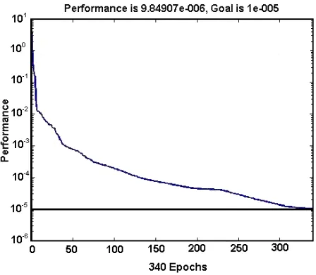
The performance of the network in training is shown in Fig. 9. The goal for the training was set to 10-5. This ensured a satisfactory response. From all the networks trained, few ones could provide this condition, from which the simplest network was chosen. To have a more precise investigation into the model, a regression analysis of outputs and desired targets was performed as shown in (Figs. 10 to 11). There is a high correlation between the predicted values by the ANN model and the measured values resulted from experimental tests. The correlation coefficient was 0.999 in the analysis of the whole network, which implies that the model succeeded in prediction of the engine performance. The data shown in Figs. 9, 10 and 11 are the experimental data presented in Figs. 4, 5 and 6. Total of 42 samples were used in this model, 80% of data (34 samples)set was randomly assigned as the training set, while the remaining 20% of data (8 samples)are put aside for prediction and validation.

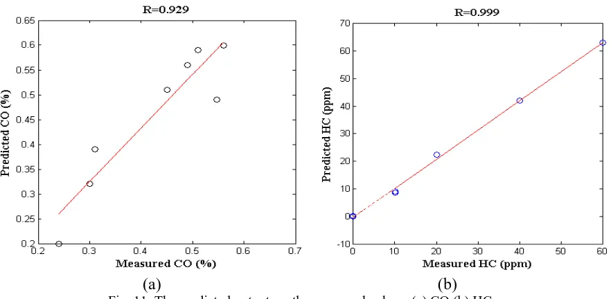
There is a strong correlation in modeling engine torque as depicted in (Fig. 10a). It is derived from the Fig. 10 that one can definitely predict engine torque and SFC separately using the designed network. It is also observed in Fig. 11 that the ANN provided the best accuracy in modeling the emission indices (HC and CO). Generally, the artificial neural network offers the advantage of being fast, accurate and reliable in predicting results, especially when numerical and mathematical methods fail. There is also a significant simplicity in using ANN due to its power to deal with multivariate and complicated problems. It was found that the R (R: correlation coefficient) values are 0.9487, 0.999, 0.929 and 0.999 for the engine torque, SFC, CO and HC emissions respectively. The simulated values by the model were obtained as 0.0004 of MSE (Mean Square Error) error.

(a) (b)

Fig. 10.The predicted output vs. the measured values, (a) engine torque (b) SFC

(a) (b)

Fig. 11.The predicted output vs. the measured values, (a) CO (b) HC

(a) (b)

Fig. 12.The trained outputs vs. measured values, (a) engine torque (b) SFC

(a) (b)

Fig. 13.The trained outputs vs. measured values, (a) CO (b) HC

5. Conclusion

to one for torque, SFC, CO and HC, while the MSE error was 0.0004. Analysis of the experimental data by the ANN revealed that there is a good correlation between the predicted data resulted from the ANN and measured ones. Therefore the ANN proved to be a desirable prediction method in the evaluation of engine parameters. There is also a priority in using artificial neural networks, since other mathematical and numerical algorithms might fail due to the complexity and multivariate nature of the problem. Generally speaking, ANN provided accuracy and simplicity in the analysis of the engine performance.

Acknowledgements

The authors would like to thank Mega Motors Company and University of Southern Queensland – Australia for providing facilities during the course of this study.

References

[1] Ma F, Hanna M A. Biodiesel production: a review. Bioresource technology 1999; 70: 1-15.

[2] Schumacher L G, Peterson C L, Grepen J V. Fuelling direct diesel engines with 2 % biodiesel blend. Written for presentation at the 2001 annual international meeting sponsored by ASAE 2001.

[3] Ghobadian B, Rahimi H. Biofuels-past, present and future perspective. International Iran and Russian congress of agricultural and natural science. Shahre cord university. Shahre cord Iran 2004.

[4] Fukuda H., Kondo A, Noda H. Biodiesel fuel production by transesterification of oils. Bioscience and bioengineering. 2001; 92: 405-416.

[5] Anonymous. European bioenergy networks. Available on the http:\\www.vtt.fi. ; 2003. [6] Lee S W, Herage T, Young B. Emission reduction potential from the combustion of soy

methyl ester fuel blended with petroleum distillate fuel. Fuel 2004; 83: 1607-1613.

[7] Wibulswas P. Combustion of blend between plant oil and diesel oil. Renewable energy [on-line]. 1999; 16: 1097 – 1101. Available on the URL: http: //WWW. Science direct.com/.

[8] Ghobadian B, Najafi G H, Rahimi H, Yusaf T F. Future of renewable energies in Iran. Renewable and Sustainable Energy Reviews 2008; article in press.

[9] Al-Widyan M I, Al-Shyoukh A O. Experimental evaluation of the transesterification of waste palm oil into biodiesel. Bioresource technology 2002; 85: 253-256.

[10] Bickel K, Strebig K. Soy-Based diesel fuel study. University of Minnesota (diesel research); 2000.

[11] Chou J, McLeod D, Pozar M, Yee J, Yeung A. UBC biodiesel initiative: helping communities to help their future; 2003 UBC seeds development studies.

[12] Leung D Y C, Koo B C P. Biodiesel – Is It Feasible to Be Used in Hong Kong? Vehicle exhausts treatment technology and control 2000; 133-138.

[13] Hertz J, Krogh A, Palmer R G. Introduction to the Theory of Neural Computation. Addison-Wesley Publishing Company, Redwood City, NJ 1991.

[15] Kalogirou SA. Application of artificial neural-networks for energy systems. Applied Energy 2000; 67: 17–35.

[16] Pacheco-Vega A, Sen M, Yang KT, McClain RL. Neural network analysis of fin-tube refrigerating heat exchanger with limited experimental data. International Journal of Heat Mass Transfer 2001; 44: 763–770.

[17] Bechtler H, Browne MW, Bansal PK, Kecman V. Neural networks – a new approach to model vapor-compression heat pumps. International Journal of Energy Research 2001:25: 591– 599.

[18] Prieto MM, Montanes E, Menendez O. Power plant condenser performance forecasting using a non-fully connected ANN. Energy 2001;26: 65–79.

[19] Chouai A, Laugeier S, Richon D. Modeling of thermodynamic properties using neural networks – application to refrigerants. Fluid Phase Equilibria 2002; 199: 53–62.

[20] Sozen A, Arcaklioglu E, Ozalp M. A new approach to thermodynamic analysis of ejector-absorption cycle: artificial neural networks. Applied Thermal Engineering 2003; 23: 937–952.

[21] Arcaklioglu E. Performance comparison of CFCs with their substitutes using artificial neural network. International Journal of Energy Research 2004; 28: 1113–1125.

[22] Ertunc HM, Hosoz M. Artificial neural network analysis of a refrigeration system with an evaporative condenser. Applied Thermal Engineering 2006; 26: 627–635.

[23] Hosoz M, Ertunc HM. Artificial neural network analysis of an automobile air conditioning system. Energy Conversion and Management 2006; 47:1574–1587.

[24] Kalogirou S A, Panteliou S. Thermosiphon solar domestic water heating systems: long-term performance prediction using artificial Neural Networks. Solar Energy2000; 69: 163–174.

[25] Canakc M I, Erdil A, Arcaklioglu E. Performance and exhaust emissions of a biodiesel engine. Applied Energy 2006; 83: 594–605.

[26] Arcaklioglu E, Celikten I. A diesel engine’s performance and exhaust emissions. Applied Energy 2005; 80: 11–22.

[27] Celik V, Arcaklioglu E. Performance maps of a diesel engine, Applied Energy 2005; 81: 247–259.

[28] Golcu M, Sekmen Y, Erduranli P, Salman S. Artificial neural network based modeling of variable valve-timing in a spark ignition engine. Applied Energy 2005; 81: 187–197. [29] Haykin S. Neural Networks: A Comprehensive Foundation, Mac-millan, New York.

1994.

[30] Chouai A, Laugier S, Richon D. Modeling of thermodynamic properties using neural networks. Application to Refrigerants Fluid Phase Equilibria 2002; 49: 1-10.

[31] Marquardt D. An algorithm for least squares estimation of non-linear parameters. Journal of the Society for Industrial and Applied Mathematics 1963; 431-441.

[32] Attiti R. First and second order methods for learning: between steepest descent and Newton's method. Neural Computing 1992; 4 (2): 141-166.