Deriving land use and land cover maps from 2.5m SPOT 5 imagery

University of Southern Queensland

Faculty of Engineering and Surveying

Deriving Land Use and Land Cover Maps

from 2.5m SPOT 5 Imagery

A dissertation submitted by

Geoffrey Michael Long

in fulfilment of the requirements of

Courses ENG4111 and 4112 Research Project

towards the degree of

Graduate Diploma of Geomatic Studies

(Geographic Information Systems)

i

Abstract

The major component in creating land use and land cover maps is satellite imagery. Currently resolutions of up to 25m imagery are used to create these maps. With the availability of higher resolution satellite imagery this dissertation investigates the classification of land use and land cover from a remotely sensed SPOT-5, 2.5m resolution colour image.

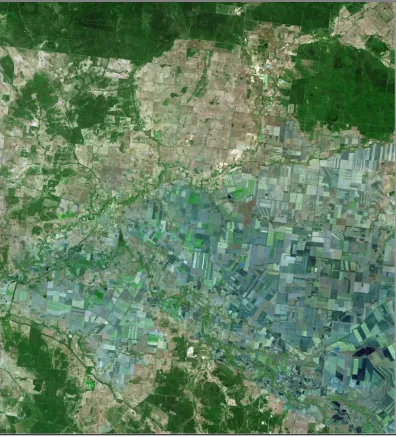
The satellite imagery used in this study was supplied by the Condamine Alliance, a regional natural resources management body. The image is covers a 60km by 60km area of the western Darling Downs region of Queensland. This area is predominately used for agricultural and grazing.

Classification of the SPOT-5 image will be accomplished using pixel-based classification methods. These will include both supervised and unsupervised classification techniques. Classification was accomplished using Idrsi Andes Image processing software.

iii

Certification

I certify that the ideas, designs and experimental work, results, analyses and conclusions set out in this dissertation are entirely my own effort, except where otherwise indicated and acknowledged.

I further certify that the work is original and has not been previously submitted for assessment in any other course or institution, except where specifically stated.

Geoffrey Michael Long

Student Number: 0050066759

Signature

28 October 2008

iv

Acknowledgements

v

Table of Contents

Abstract ... i

Disclaimer ... iii

Certification... iii

Acknowledgements ... iv

List of Figures ... viiii

List of Tables... ix

Abbreviations ... x

Chapter 1 - Introduction 1.1 Introduction ... 1

1.2 Aims / Objectives ... 4

1.3 Conclusion: Chapter 1 ... 4

Chapter 2 - Literature Review 2.1 Introduction ... 5

2.2 Land Cover / Land Use Mapping ... 5

2.2.1 Background ... 5

2.2.2 Data ... 6

2.2.3 Methods of Classification ... 6

2.2.4 Accuracy Assessment ... 9

2.3 Land Cover and Land Use Mapping in Queensland ... 9

2.3.1 Background ... 9

2.3.2 SLATS ... 9

2.3.3 SLATS - Land Cover Mapping Methodology ... 11

2.3.4 QLUMP ... 11

2.3.5 QLUMP - Land Use Mapping Methodology ... 13

2.4 Summary: Chapter 2 ... 14

Chapter 3 - Research and Methodology 3.1 Introduction ... 15

3.2 Image Interpretation ... 15

vi

3.3.1 Unsupervised Classification ... 19

3.3.2 Development of Training Samples ... 27

3.3.2 Supervised Classification ... 32

3.4 Conclusion: Chapter 3 ... 32

Chapter 4 - Analysis of Results 4.1 Introduction ... 33

4.2 Unsupervised Classification Results ... 33

4.2.1 Four Cluster Unsupervised Classification ... 33

4.2.2 Ten Cluster Unsupervised Classification ... 35

4.3 Supervised Classification Results... 36

4.3.1 Parallelepiped Classification... 36

4.3.2 Maximum Likelihood Classification ... 37

4.3.3 Nearest-Neighbour Classification ... 38

4.3.4 Multi-layer Perceptron Classification ... 39

4.4 Accuracy Assessment ... 40

4.5 Conclusion: Chapter 4 ... 45

Chapter 5 - Conclusions 5.1 Introduction ... 46

5.2 Conclusion ... 46

References ... 48

Appendix A - Project Specification ... 50

vii

List of Figures

Figure 1-1: Extent of SPOT-5 Image over the Condamine River Catchment 2

Figure 1-2: SPOT-5 Image 3

Figure 2-1: Land Cover of Queensland 10

Figure 2-2: Land Use Map of Queensland 12

Figure 3-1: Visual Interpretation of SPOT-5 Image 16 Figure 3-2: Greyscale Images for Red, Green and Blue Bands 17

Figure 3-3: Histogram of the Red Band 17

Figure 3-4: Histogram of the Green Band 18

Figure 3-5: Histogram of the Blue Band 18

Figure 3-6: Isocluster Histogram 19

Figure 3-7: Unsupervised Classification – Isocluster (10 Clusters) 20 Figure 3-8: Isocluster (10 Clusters) Results – Clusters 1 - 4 21 Figure 3-8: Isocluster (10 Clusters) Results – Clusters 5 - 8 22 Figure 3-8: Isocluster (10 Clusters) Results – Clusters 9 - 10 23

Figure 3-9: Combination of Clusters 23

Figure 3-10: Unsupervised Classification – Isocluster (4 Clusters) 25 Figure 3-11: Isocluster (4 Clusters) Results – Clusters 1 - 4 26

Figure 3-12: Example of Land Cover - Trees 27

Figure 3-13: Examples of Land Cover - Water 28 Figure 3-14: Example of Land Cover - Structures 29 Figure 3-15: Example of Land Cover - Pasture 30

viii Figure 4-1: Unsupervised Classification – Four Clusters 34 Figure 4-2: Unsupervised Classification – Ten Clusters 35 Figure 4-3: Supervised Classification - Parallelepiped 36 Figure 4-4: Supervised Classification – Maximum Likelihood 37 Figure 4-5: Supervised Classification – Nearest Neighbour 38 Figure 4-6: Supervised Classification – Multi-Layer Perceptron 39

Figure 4-7: SLATS Land Cover Map 42

ix

List of Tables

Table 4-1: Comparison of Overall Accuracy for Classification Techniques 41 Table 4-2: Accuracy Results for Maximum Likelihood Classification 41

x

Abbreviations

ACLUMP Australian Collaborative Land Use Mapping Program

FAO Food and Agriculture Organization of the United Nations

NRW Department of Natural Resources and Water

QLUMP Queensland Land Use Mapping Program

1

Chapter 1

INTRODUCTION

1.1 Introduction

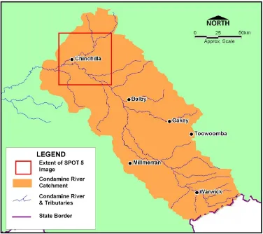
The importance of accurate land cover and land use maps is ever increasing with the current environmental challenges facing the population. This project investigates the classification of high resolution satellite imagery to create land cover and land use maps. For this project a SPOT-5, 2.5m resolution colour image was sourced from the Condamine Alliance. Figure 1-1 shows the extent of the SPOT-5 satellite image over the Condamine River catchment.

2

Figure 1-1: Extent of SPOT-5 Image over the Condamine River catchment.

3

4

1.2 Aims / Objectives

Satellite imagery is the major component in the development of land cover and land use maps. The current methods used to produce land cover and land use maps utilise satellite imagery at resolutions of 25m. Now that high resolution satellite imagery is becoming more readily available further study needs to be completed to see its worth in assisting in production of land cover and land use maps.

The aim of this project is to produce standard procedures to derive land cover and land use maps from SPOT-5 imagery. Experiments with different classification techniques will be investigated and documented to enable comparisons that will demonstrate what technique is most effective.

To derive land cover / land use maps from SPOT-5 2.5m satellite imagery the following objectives were identified:

Research image classification techniques for SPOT-5 satellite imagery. Investigate current methods of land cover / land use mapping in Queensland. Experiment with different image classification methods and analyse results. Determine accuracy of produced land cover maps and compare with currently available map.

1.3

Conclusions: Chapter 1.

5

Chapter 2

LITERATURE REVIEW

2.1

Introduction

This chapter investigates methods of creating land cover and land use maps. It looks at the data used in land cover mapping and overviews the methods of classifying remotely sensed imagery focusing on SPOT-5 satellite imagery. It also looks at measuring the accuracy of the classified image

Also provided is a summary of land use and land cover mapping in Queensland. Description of the land cover and land use maps are provided to establish the different information they each provide. Methodologies for how both land cover and land use maps are derived are covered separately.

2.2

Land Cover / Land Use Mapping

2.2.1 Background

6 2.2.2 Data

Remotely sensed image sources to create land cover and land use maps are many and varied. The more local the area to be classified the higher resolution imagery is needed. For local areas imagery from IKONOS, Quickbird, and SPOT-5 HRG are most useful (Lu and Weng 2005).

To assist in the classification process and obtain accuracy measures other satellite imagery, existing maps, fieldwork, aerial photography are utilised. This information is used as a basis for training sites and to determine image classification accuracy.

2.2.3 Methods of Classification

Image classification is needed to create land cover and land use maps from remotely sensed imagery. There are two systems to classifying land cover / land use, a priori

and a posteriori (Di Gregorio 1996). These are more commonly known as supervised

and unsupervised classification techniques.

Unsupervised classification uses a process of clustering. Mather (2004) sees this as ‘a kind of exploratory procedure’, to determine the number of categories within an image and assign the pixels to them. Examples of unsupervised classification methods are ISODATA and K-means (Leu and Weng 2005).

7

classification methods are maximum likelihood, minimum distance, decision tree, and artificial neural network (Leu and Weng 2005).

Most important to supervised classification are training samples and their representation within the image (Mather 2004). Training samples are usually created from fieldwork, aerial photography, and existing maps. Visual interpretation can be used to find the training samples position within the image (Mather 2004). Mather (2004) also states that the reliability and representativeness of the training sample has a considerable affect on the performance of neural and statistical classifiers.

Research shows there are many different methods used to classify SPOT-5 satellite imagery. An article by Wang et al. (2008) investigates object-oriented classification. The object-oriented or object-based classification approach segments an image into objects. It does this by merging similar pixels. While their results were good, classification accuracy up to 87%, their study did not contain a comparison with pixel-based methods over the same image. Ivits et al. (2005) investigated pixel-based and object-based classification methods. Their results showed similar performance in accuracy for classifying land cover from SPOT-5 imagery for both pixel- and object-based classification methods.

8

For this project both supervised and unsupervised classification methods are used. Techniques such as parallelepiped, maximum likelihood, nearest-neighbour, and neural networks will be compared to determine the most effective for SPOT-5 2.5m colour image classification.

2.2.4 Accuracy Assessment

Once the image is classified a measure of accuracy needs to be established. Mather (2004) states that the k × k confusion (or error) matrix is the most commonly used method to show the accuracy of classification. Sample data is compared against referenced data.

A study by Lui, Frazier and Kumar (2007) compared fourteen category measures and twenty map measures. They recommended that the ‘user’s’ and ‘producer’s’ accuracy be used for category measurement accuracy and that the ‘overall’ accuracy measure be used for map accuracy. User’s accuracy measures the probability that a sample of the classified pixels is classified correctly whereas producer’s accuracy measures the probability that the reference data will be classified correctly (Nishii & Tanaka 1999). Overall accuracy is determined by dividing the correctly classified pixels by the total number of sample pixels.

9

2.3

Land Cover / Land Use Mapping in Queensland

2.3.1 Background

In Queensland the Department of Natural Resources and Water (NRW) manage two projects for land cover and land use mapping. The land cover mapping project categorises the makeup of the earth’s surface, whereas the land use mapping project categorises what the land is used for.

The Statewide Landcover and Trees Survey (SLATS) project produces land cover maps, and the Queensland Land Use Mapping Program (QLUMP) is responsible for land use mapping in Queensland.

2.3.2 SLATS

In Queensland the Statewide Landcover and Trees Survey (SLATS) project produces land cover maps. The primary objective of the SLATS project is to monitor land cover change. This project was initiated by the Queensland Government in response to the atmospheres build up of greenhouse gases.

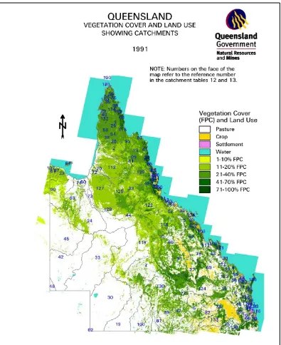
The land cover maps are created from remotely sensed satellite imagery. Currently SLATS uses six categories of land cover; trees, pasture, crop, water, settlement, and other. Figure 2-1 shows a land cover map of Queensland.

While there have been moves to introduce a national classification scheme for land cover mapping, the National Land and Water Resources Audit convened a land cover workshop in July 2007, this is still an on going concern.

10

11 2.3.3 SLATS - Land Cover Mapping Methodology

Satellite remote sensing is the basis for SLATS land cover determination. A mosaic of 185km by 185km Landsat images is created to cover the whole of Queensland. SLATS has two main parts to mapping land cover. The first is to separate wooded and forested areas from other types of land cover, the second is to estimate tree density of the wooded/forested areas (Kuhnell et al. 1998). For this research project only the determination of land cover is to be investigated.

SLATS uses both supervised and unsupervised techniques to determine land cover types. Supervised classification techniques utilise external information to assist in classification, this may include fieldwork, aerial photography, reports and other maps. Unsupervised classification determines classes without the aid of external information (Mather, 2004).

For supervised classification SLATS use site data, visual observations, and aerial photography. Spectral signatures of different land cover types are used to assist in determining whether an area is wooded (Kuhnell et al. 1998).

2.3.4 QLUMP

Land use mapping categorises areas into what the land is used for. Until recently land use mapping was only create for specific projects targeting only on its areas of interest. The categories used for land use mapping were project specific; this made it difficult to compare areas with one another.

12

There are three levels of land use classification, primary, secondary, and tertiary. The six primary land use categories are conservation and natural environments, production from relatively natural environments, production from dryland agriculture and plantations, production from irrigated agriculture and plantations, intensive uses, and water. Figure 2-2 shows the primary land use coverage for Queensland.

13 2.3.5 QLUMP - Land Use Mapping Methodology

To create land use maps, QLUMP first collates information for each catchment from available existing datasets. There are three classifications of datasets, image, primary and ancillary data. Image Data includes Landsat ETM+ imagery, aerial photography and high resolution satellite imagery. Land cover maps produced by SLATS, digital cadastral maps, valuation and sales data, state forest and timber reserves, national parks, and waterbodies are the primary data. Additional datasets are used depending on individual catchment requirements, these could include soil maps, crop data and local council provided information (Witte et al. 2006).

A draft map is produced from the primary data integrated into a model using Erdas Imagine software. Each pixel is classified through a decision process. The output pixel size is at a 25m resolution. The next step is image interpretation. Here the draft land use map is edited in the Erdas Imagine software utilising the Landsat image as a background. Aerial photography is used to assist in interpreting land use classifications.

Once the second draft is complete the map is verified and expert knowledge is utilised to refine the data contained in the land use map. This is entered into the model making necessary adjustments. The map is now ready to be assessed for accuracy. The data is validated uses expert knowledge and fieldwork. In some instances surveys of property owners are conducted to ensure the integrity of the land use data.

14

2.4

Summary: Chapter 2

15

Chapter 3

RESEARCH AND METHODOLOGY

3.1 Introduction

This chapter investigates the image and its relationship with real world features. Image interpretation is completed by visual interpretation and using Idrisi Andes image processing software.

The remotely sensed image classified is a SPOT-5 2.5m resolution colour image. This image covers a 60km x 60km area of rural Queensland. The image format is an ECW file that has been georeferenced.

The ECW file was imported into the Idrisi Andes imaging software. The software converts the file into 3 bands, red, green, blue and a composite RGB file. Firstly the composition of the image was analysed to identify features.

Unsupervised classification was performed using the Idrisi Andes Isocluster function. The Isocluster function is a similar algorithm to isodata, developed by Ball and Hall (1965). Examples of results from both four cluster and 10 cluster experiments are presented.

Included in this chapter is the development of training samples for supervised classification.

3.2 Image Interpretation

16

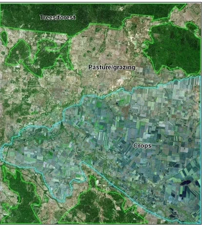
areas of forest/trees, crops, and pasture/grazing lands. Theses areas are shown in figure 3-1, forest/trees are outlined in green, crops are outlined in blue, and the areas in between are grazing. On zooming in on the image other type land cover types such as water and man-made structures are visible, however these areas are quite small within the whole extents of the image.

17

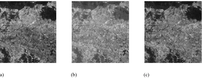
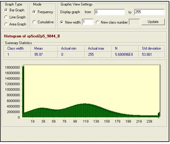
The greyscale images for each of the band can be seen in figure 3-2. The red and blue bands appear very similar, with the red band having a slightly higher contrast in the crops area. The green band appears faded relative to the other two bands. Histograms for bands are shown in figures 3-3, 3-4, and 3-5. The range of values for all bands was from 0 to 255.

(a) (b) (c)

Figure 3-2: SPOT-5 greyscale images for each band, (a) red, (b) green, and (c) green.

18

Figure 3-4: Histogram of green band

19

3.3 Classification

3.3.1 Unsupervised Classification

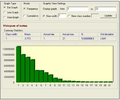
Different methods of classification used. Exploratory classification was first used to determine the most effective number of clusters. The isocluster function clustered the data into 21 separate classes. The resulting histogram, figure 3-6, shows that there are four main classes, and another six substantially sized classes. This class division will assist in determining the number of clusters for unsupervised classification and the number of training samples to develop for supervised classification.

20

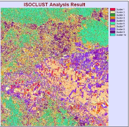
Figure 3-7 shows the results of using 10 clusters and figure 3-11 shows the results of using 4 clusters.

Figure 3-7: Results of Isocluster with 10 clusters

21

9 and to a lesser extent clusters 2 and 4 best represent the grazing areas. Cluster 1 provides small areas that could be added to the crops clusters.

(a) Cluster 1 (b) Cluster 2

(c) Cluster 3 (d) Cluster 4

22

(e) Cluster 5 (f) Cluster 6

(g) Cluster 7 (h) Cluster 8

23

(i) Cluster 9 (j) Cluster 10

Figure 3-8: Isocluster results (i) and (j)

Combining the clusters provide clearer results for each of the main land covers. While cluster 1 was most aligned with the crops area it was not combined with any other clusters due to its varied results. Figure 3-9 shows the results of combining clusters that represent similar land covers. The clustering procedure for treed area and the crop area land covers appear highly successful.

(a) (b) (c)

24

25

26

(a) (b)

(c) (d)

Figure 3-11: Separate results for the isocluster function with four clusters. Cluster 1 (a) and cluster 4 (d) cover areas of grazing and crops. Cluster 3 (c) mainly covers the treed areas and cluster 2 (b)

27 3.3.2 Development of Training Samples

Unsupervised classification produced three main clusters that were identifiable with land cover. These were the trees/forest, grazing/pasture, and crop areas. For this project at least five classes of land cover are desirable so the inclusion of urban and water areas are required.

Training samples were developed for five different classes to determine five different land cover types. The land cover types chosen were trees/forest, crops, grazing/pasture, urban, and water.

Areas of heavy forestation, figure 3-12, were used as training sites for the trees/forest land cover class. Care was taken to ensure training sites did not cross over any roads, tracks, buildings, any other objects that may interfere with the integrity of the sample data.

28

The locality of the satellite image contains very little areas of water; some waterways contain visible water however most streams are delineated by trees. Water that is visible in the image mainly appears as two different colours, cyan and black, see figure 3-13. The cyan coloured water areas are confined to mostly farm dams. The black coloured water areas are larger watercourses. Two categories of water are used as training samples.

(a) Dams (b) Major waterway

29

The urban areas of the image are difficult to define because of the varying pixel colours. At the 2.5m resolution structures are visible and highly reflective, areas of vegetation and roadways are also visible between the structures. This can be seen in figure 3-14.

Figure 3-14: Example of an urban area within the SPOT-5 image. Most man-made structures appear white and trees and roadway is also identifiable.

30

Open ground are the areas of grassland, grazing/pasture are very open and have few trees. Figure 3-15 shows grazing areas and its variations in colour. These areas also contain farm structures and dams. Training samples developed for grazing/pasture avoided structures, trees, and dams.

31

Agricultural areas are a patchwork of colours; this is due to type of crop is grown, the amount of irrigation, stage of growth, or it being a recently ploughed area. Due to the large variations in colour between plots sampling of different categories of crops were performed to ensure adequate coverage of all agricultural types of this area. Examples of the variable crop areas can be seen in figure 3-16.

32

Two sets of training samples were developed to explore their effectiveness in supervised classification. One set contained 5 categories of land cover that best represented the classes of the area. The second set of training samples contained 10 categories. One category of each for the trees, grazing, and urban areas, 5 categories of crops, including ploughed areas, and two categories of water made up the 10 categories.

3.3.3 Supervised Classification

Methods of supervised classification used to produce land cover maps are parallelepiped, maximum likelihood, nearest-neighbour, and multi-layer perceptron techniques. For each method of classification both sets of training samples were used to provide comparisons. All image classification was processed through Idrisi Andes image processing software.

3.4

Conclusion: Chapter 3

33

Chapter 4

Analysis of Results

4.1

Introduction

This chapter investigates the results of the image classification techniques and determines their accuracy. Analyses of errors are investigated with reasons and possible areas for improvement are explored. This chapter also determines the best pixel-based classification technique for creating land cover and land use maps from SPOT-5 2.5m resolution images.

Four supervised classification techniques were experimented with and their results are compared. Each supervised classification technique used both five category and ten category training samples. Overall accuracy was assessed using random sample pixels and a k × k error matrix.

4.2

Unsupervised Classification Results

Unsupervised classification was used for exploratory purposes. Decision on the number of clusters was based on the histogram produced from the Isocluster function, figure 3-6, and the number of classes desired. The results from unsupervised classification did not reveal any other clusters than the treed, crops, and pasture areas.

4.2.1 Four Cluster Unsupervised Classification

34

put together. The result of unsupervised classification using four clusters is shown in figure 4-1.

Figure 4-1: Unsupervised classification results using four clusters.

35 4.2.2 Ten Cluster Unsupervised Classification

While the results of using ten clusters for classification was better than four the classification process it did not reveal any more than the three dominant land cover types forest/trees, agriculture, and open pasture.

36

4.3

Supervised Classification Results

4.3.1 Parallelepiped Classification

Figure 4-3 shows the results of image classification using the parallelepiped classification method with five categories of land cover.

37 4.3.2 Maximum Likelihood Classification

Figure 4-4 shows the results of image classification using the maximum likelihood classification method with ten categories of land cover. Visual interpretation shows good results for trees and pastures areas.

38 4.3.3 Nearest-Neighbour Classification

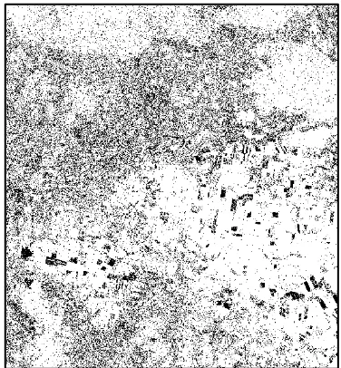
Figure 4-5 shows the results of image classification using the nearest neighbour classification method with ten categories of land cover.

39 4.3.4 Multi-layer Perceptron Classification

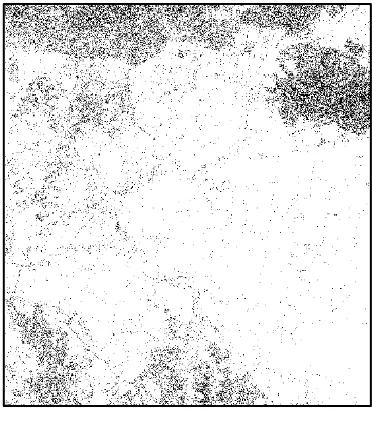
Figure 4-6 shows the results of image classification using the multi-layer perceptron classification method with five categories of land cover.

40

4.4

Accuracy of Classification

To determine the accuracy of the image classification, samples were generated and then assigned classification based on the visual interpretation of the original SPOT-5 image and Google Earth imagery. Accuracy of classification measured the land cover class only with any subclasses (categories) merged. Random samples of the classified image were generated by the Idrisi image processing software. These samples were investigated for accuracy either by re-inspection of the SPOT-5 image or inspection of Google Earth imagery. The results of the accuracy were entered into an error matrix.

An initial random sample of 300 pixels was generated. This provided 102 crop, 89 pasture, 107 treed, 1 water, and 1 urban pixels. To improve the cover of samples for water and structures stratified random sampling was attempted. This sampling technique did not improve the representation of the water and structures. Further samples were taken from the water and urban areas to provide sample pixels for accuracy assessment. A total of 397 sample pixels were used, 110 crop, 105 pasture, 126 trees, 24 water, and 32 structures.

41

Classification Method Accuracy 5 Categories

Accuracy 10 Categories

Parallelepiped 57.18% 55.67%

Maximum Likelihood 74.06% 77.33%

Nearest-Neighbour 70.78% 67.25%

Multi-Layer Perceptron 74.56% 72.79%

Table 4.1: Comparison of overall accuracy between classification methods.

Table 4-2 shows the error matrix for the maximum likelihood classifier. This classification produced an overall accuracy of 77.33%. Appendix B provides the k × k error matrix for all the classification methods.

Classified Classes Users

1 2 3 4 5 Accuracy

Ref. Data

1 79 13 4 1 10 107 73.83%

2 16 84 12 0 1 113 74.34%

3 14 6 108 2 3 133 81.20%

4 0 1 2 21 3 27 77.78%

5 1 1 0 0 15 17 88.24%

110 105 126 24 32 397 77.33%

Producers

Accuracy 71.82% 80.00% 85.71% 87.50% 46.88%

Table 4.2: Accuracy results for Maximum Likelihood Classification

42

Table 4.3: Accuracy results for SLATS land cover map

Figure 4-7: SLATS land cover map.

Classified Classes Users

Ref. Data 1 2 3 4 5 Accuracy

1 98 16 5 11 1 131 74.81%

2 10 77 24 5 4 120 64.17%

3 2 9 89 7 1 108 82.41%

4 0 3 0 1 0 4 25.00%

5 1 0 8 0 26 35 74.29%

111 105 126 24 32 398 73.12%

Producers

43

Although the maximum likelihood classification produced good results there are areas for improvement. Looking at the error matrix, table 4-2, the ‘producers’ accuracy for category 5, water, is 46.88%. This means that of the 32 referenced water pixels the classification method identified less than half of them, with nearly a third being classified as crop. Also visual interpretation of the maximum likelihood classification shows large extents of water; see the bottom right-hand area of figure 4-4. These areas are actually a type of crop.

44

45

4.5

Conclusion: Chapter 4

46

Chapter 5

Conclusions

5.1

Introduction

This project aimed to develop a standard procedure to derive accurate land cover and land use maps from 2.5m resolution SPOT-5 satellite imagery.

To accomplish this task the current methods of SPOT-5 satellite imagery classification were researched. Also, current methods of determining land cover and land use maps were investigated.

Utilising different classification methods available a procedure was devised to create a land cover map.

5.2

Conclusions

This project has shown that it is possible to derive land cover / land use maps from SPOT-5, 2.5m resolution colour satellite imagery. Experimentation with different classification methods showed that using the maximum likelihood classification is the most effective of the pixel-based classification techniques. It also shows that by dividing the classifications into categories of different spectral reflectance improved the accuracy of classification.

Using unsupervised classification resulted in determining there were three main land cover types. This showed the value of using clustering as a basis to determine the major land cover types.

47

79.59%. This filter assists in removing speckling that occurs due to spectral variations in a land cover class.

This dissertation concludes that to derive land cover / land use maps from SPOT-5 2.5m resolution colour imagery the following steps should be taken:

1. Use visual interpretation to locate land cover / land use types. 2. Use unsupervised classification to uncover any hidden classes. 3. Develop training samples for supervised classification.

4. Use maximum likelihood classification technique.

5. Undertake accuracy assessment using random samples and collating results in a k × k error matrix.

6. Carry out post-classification filtering.

48

REFERENCES

Ball, GH, and Hall, DJ, 1965, A Novel Method of Data Analysis and Pattern

Classification, Menlo Park, CA: Stanford Research Institute.

Department of Natural Resources and Mines 2004, Land Cover Change in

Queensland 1988-1991: A Statewide Landcover and Trees Study (SLATS) Report,

Brisbane.

Department of Natural Resources and Water 2007, Land Cover Change in

Queensland 2004-2005: A Statewide Landcover and Trees Study (SLATS) Report,

Brisbane.

Di Gregorio, A 1996, ‘FAO Land Cover Classification: A Dichotomous, Modular, Heirarchical Approach, Proceedings of the US Federal Geographic Data Committee

Vegetation Subcommittee and Earth Cover Working Group, 15 – 17 October 1996,

Washington, USA.

Goulevitch, BM, Danaher, TJ, Stewart, AJ, Harris, DP, and Lawrence, LJ 2002, ‘Mapping woody vegetation cover over the state of Queensland using Landsat TM and ETM+ imagery’, Proceedings of the 11th Australasian Remote Sensing and

Photogrammetry Conference, Brisbane, Australia.

Ivits, E, Hemphill, S, Langar, F, and Koch, B 2005, ‘Benchmarking of pixel- and object-based classification methods’, Geoland Project Report, University of Freiburg, Germany.

Kuhnell, CA, Goulevitch, BM, Danaher, TJ & Harris, DP 1998, ‘Mapping Woody Vegetation Cover over the State of Queensland using Landsat TM Imagery’, Proceedings of the 9th Australasian Remote Sensing and Photogrammetry

49

Liu, C, Frazier, P, and Kumar, L 2007, ‘Comparative assessment of the measures of thematic classification accuracy’, Remote Sensing of Environment, vol. 107, issue 4, 30 April 2007, pp. 606 – 616.

Lu, D and Weng, Q 2005, ‘A survey of image classification methods and techniques for improving classification performance’, International Journal of Remote Sensing, vol. 28, no. 5, 10 March 2007, pp. 823-870.

Mather, PM 2004, Computer Processing of Remotely-Sensed Images An Introduction, 3rd edn, John Wiley & Sons, West Sussex, England.

Nishii, R, and Tanaka, S 1999, ‘Accuracy and inaccuracy assessments in land-cover classification’, Geoscience and Remote Sensing, vol. 37, issue 1, part 2, January 1999, pp. 491-498.

Wang, Z, Wei, W, Zhao, S, Chen, X 2004, ‘Object-oriented classification and application in land use classification using SPOT-5 PAN imagery, Proceedings of the

Geoscience and Remote Sensing Symposium 2004, IGARSS ’04, vol. 5, September

2004, pp. 3158 – 3160.

Witte, C, van den Berg, D, Rowland, T, O’Donald, T, Denham, R, Pitt, G & Simpson, J 2006, Mapping Land Use: Technical Report on the 1999 Land Use Data

50

Appendix A

52

Appendix B

53

Parallelepiped 5 Categories

Classified Users

Ref. Data 1 2 3 4 5 Accuracy

1 20 4 11 0 5 40 50.00%

2 74 81 13 0 3 171 47.37%

3 3 1 96 2 2 104 92.31%

4 0 0 0 10 0 10 100.00%

5 8 12 1 1 20 42 47.62%

Not Classified 5 7 5 11 2 30

110 105 126 24 32 397 57.18%

Producers

Accuracy 18.18% 77.14% 76.19% 41.67% 62.50%

Parallelepiped 10 Categories

Classified Users

Ref. Data 1 2 3 4 5 Accuracy

1 27 6 12 1 1 47 57.45%

2 59 86 11 0 3 159 54.09%

3 1 0 85 1 2 89 95.51%

4 0 1 1 15 0 17 88.24%

5 0 0 0 0 8 8 100.00%

Not Classified 23 12 17 7 18 77

110 105 126 24 32 397 55.67%

Producers

54

Maximum Likelihood 5 Categories

Classified Users

Ref. Data 1 2 3 4 5 Accuracy

1 82 23 14 2 8 129 63.57%

2 17 77 8 0 0 102 75.49%

3 4 1 102 7 3 117 87.18%

4 0 0 0 14 2 16 87.50%

5 7 4 2 1 19 33 57.58%

110 105 126 24 32 397 74.06%

Producers

Accuracy 74.55% 78.79% 75.40% 58.33% 59.38%

Maximum Likelihood 10 Categories

Classified Users

Ref. Data 1 2 3 4 5 Accuracy

1 79 13 4 1 10 107 73.83%

2 16 84 12 0 1 113 74.34%

3 14 6 108 2 3 133 81.20%

4 0 1 2 21 3 27 77.78%

5 1 1 0 0 15 17 88.24%

110 105 126 24 32 397 77.33%

Producers

55

Nearest Neighbour 5 Categories

Classified Users

Ref. Data 1 2 3 4 5 Accuracy

1 76 23 19 1 8 127 59.84%

2 27 77 9 1 3 117 65.81%

3 5 1 97 9 2 114 85.09%

4 0 0 0 13 1 14 92.86%

5 2 4 1 0 18 25 72.00%

110 105 126 24 32 397 70.78%

Producers

Accuracy 69.09% 73.33% 76.98% 54.17% 56.25%

Nearest Neighbour 10 Categories

Classified Users

Ref. Data 1 2 3 4 5 Accuracy

1 102 48 34 3 11 198 51.52%

2 6 46 4 0 0 56 82.14%

3 0 0 80 1 2 83 96.39%

4 0 1 7 20 0 28 71.43%

5 2 10 1 0 19 32 59.38%

110 105 126 24 32 397 67.25%

Producers

Accuracy 92.73% 43.81% 63.49% 83.33% 59.38%

56

Multi-Layer Perceptron 5 Categories

Classified Users

Ref. Data 1 2 3 4 5 Accuracy

1 80 10 12 9 12 123 65.04%

2 20 91 16 0 1 128 71.09%

3 6 2 97 2 3 110 88.18%

4 0 0 0 13 1 14 92.86%

5 4 2 1 0 15 22 68.18%

110 105 126 24 32 397 74.56%

Producers

Accuracy 72.73% 86.67% 76.98% 54.17% 46.88%

Multi-Layer Perceptron 10 Categories

Classified Users

Ref. Data 1 2 3 4 5 Accuracy

1 83 12 18 12 13 138 60.14%

2 18 86 15 0 1 120 71.67%

3 1 0 91 1 2 95 95.79%

4 0 0 1 11 0 12 91.67%

5 8 7 1 0 16 32 50.00%

110 105 126 24 32 397 72.79%

Producers