OPC cycle time analyser

University of Southern Queensland

Faculty of Engineering and Surveying

OPC Cycle Time Analyser

A dissertation submitted by

Clement Bollaart

In the fulfilment of requirements of

Courses ENG4111 and 4112 Research Project

towards a degree of

Bachelor of Electronics and Computing Engineering

Abstract

Variations in equipment cycle times can have a significant effect on the output of

modern assembly lines. In an effort to identify and act accordingly when these

variations occur, the development of a software application to analyse equipment

cycle time via OPC is investigated in this project.

Manufacturing organisations continuously seek improvements in equipment

performance and output. A common improvement made is the reduction of

equipment cycle time, this provides an increase in output for a relatively small

capital outlay. These improvements remain relatively unchecked and variations in

cycle time due to numerous factors continue to influence equipment performance.

An equipment cycle time analyser can be used to monitor and report variations in

cycle time. The resulting information can be used to predict equipment failures and

allow maintenance departments to plan corrective actions. This analyser tool can

also be used by engineering departments for analysing equipment cycle time during

cycle time improvement projects and new equipment installation.

Currently the development of the cycle time analyser system is at a stage where the

cycle time of equipment can be monitored using OPC as a means of communication.

Additionally a Microsoft Excel application is available which can import the data

recorded by the cycle time analyser software and display a step time diagram of a

Certification

I certify that the ideas, designs and experimental work, results, analyses and

conclusions set out in this dissertation are entirely my own effort, except where

otherwise indicated and acknowledged.

I further certify that the work is original and has not been previously submitted for

assessment in any other course or institution, except where specifically stated.

Clement Christiaan Bollaart

Student Number: 0050029162

Signature

11

October 2007

Acknowledgements

I would like to thank the following people for their assistance and support which

have contributed greatly to the success of this project.

Dr. Peng (Paul) Wen (supervisor) for his guidance and constructive criticism given

during this project.

My colleagues and managers from Robert Bosch (Australia) for their support,

understanding and assistance during the project term.

T

able of Contents

Abstract

ii

Limitations of Use

iii

Certification

iv

Acknowledgements

v

Table of Contents

vi

List of Figures

viii

List of Tables

viii

Definitions

ix

Chapter 1 Introduction ...11

1.1 Project Aim...11

1.2 Project Objectives ...12

1.3 Chapter Overview ...13

1.4 Chapter Summary ...14

Chapter 2 Background ...15

2.1 History of Lean Manufacturing ...15

2.2 Line Balancing...15

2.3 Trends in Current Manufacturing ...17

2.4 Current Cycle Time Data...19

2.5 Real Time Data via OPC ...20

2.6 TPM and Predictive Maintenance...21

2.7 Benchmarking...22

2.8 Summary...23

Chapter 3 Methodology ...25

3.1 Overview ...25

3.2 Design Process Model...25

3.3 Communication with OPC Server...26

3.4 Development of User Interface...26

3.5 Design and Implementation of Reports...27

3.6 Programming Language Selection...27

3.7 Analysis of Cycle Times ...28

3.7.1 Machine Capability ... 28

3.7.2 Simplified Machine Capability ... 29

3.7.2 Example Tolerance Calculation. ... 30

3.8 Chapter Summary ...31

Chapter 4 System Development and Implementation...32

4.1 Overall Description ...32

4.2 OPC Communication ...32

4.3 OPC OPCDAAUTO.DLL ...33

4.4 User Permission Considerations ...34

4.5 DCOM Setting Required ...35

4.6 Recording Format ...35

4.7 Operation of Cycle Time Analyser Software ...36

4.7.1 Connection to OPC Server... 37

4.7.2 Create OPC group ... 38

4.7.3 Add OPC Items to Group ... 38

4.7.4 Start Recording... 39

4.7.6 User Instructions ... 41

4.8 Testing ...41

4.9 Visualisation of Recorded Data ...42

4.10 Visual Basic Limitations ...43

4.11 Problems Encountered...44

4.11.1 OPC TimeStamp... 44

4.11.2 DCOM Security Settings ... 45

4.11.3 SyncRead does not Return Timestamp Data as Array ... 46

4.11.4 OPC Server Capability ... 47

4.12 Chapter Summary...47

Chapter 5 Conclusions ...48

5.1 Achievement of Objectives ...48

5.2 Future Work...49

5.2.1 Statistical Evaluation of Tolerance Times... 49

5.2.2 Monitor Multiple Machines ... 49

5.3 Final Summary...50

References...51

Appendix A...52

Project Specification ...52

Appendix B ...54

OPC Input Items Example ...54

Appendix C ...55

Cycle Time Analyser Instruction Manual ...55

Appendix D...76

DCOM Setting for windows XP...76

Appendix E ...86

OPC Tunneller Quotation ...86

Appendix F...88

Visual Basic Code...88

List of Figures

FIGURE 1: HENRY FORD (1919) 15

FIGURE 2: FORD ASSEMBLY LINE 15

FIGURE 3: LINE BALANCING WORKSHEET 16

FIGURE 4: HIGH FLEXIBILITY PRODUCTION LINE 18

FIGURE 5: CYCLE TIME STATISTICS – TYPICAL MANUFACTURING DATA 19

FIGURE 6: PDCA CYCLE 22

FIGURE 7: TYPICAL “ACL” ENTRY 26

FIGURE 8: NORMAL DISTRIBUTION 29

FIGURE 9: MACHINE CAPABILITY PROCESS FLOW 30

FIGURE 10: ARCHITECTURE OF THE CODESYS OPC SERVER 33

FIGURE 11: INTERFACING TO OPC SERVERS 34

FIGURE 12: VISUAL BASIC DATA ARRAY 35

FIGURE 13: TEXT FILE FORMAT 36

FIGURE 14: OPC VISUALISATION 36

FIGURE 15: SERVER CONNECT 37

FIGURE 16: GROUP CONNECT 38

FIGURE 17: ADD ITEMS 39

FIGURE 18: FUNCTION BUTTONS 40

FIGURE 19: RESULTS DISPLAY 40

FIGURE 20: EXCEL REPORT 43

FIGURE 21: CODE FOR MILLISECOND CONVERSION 45

List of Tables

Definitions

Client – Computers or applications that employ the services of Servers.

Cm, Cmk – Machine capability index

COM – Component Object Model, which supports communication among

objects on different computers.

DCOM – Distributed COM

LSL – Lower Stability Limit

MUDA – Waste (non value added)

OLE – Object Linking and Embedding

OPC – OLE for Process Control

PPM – Parts Per Million

RAD – Rapid Application Development, an incremental software process

model that emphasizes a short development cycle.

Server – Device which centrally provides certain services within a network.

TCP/IP – Transmission Control Protocol / Internet Protocol, the set of rules

which controls virtually the entire communications over the internet and also

applies to most separate networks.

TPM - Total Productive Maintenance

TPS – Toyota Production Systems

UTC – Coordinated Universal Time, UTC-based time is loosely defined as the

current date and time of day in Greenwich, England

USL – Upper Stability Limit

LSL – Lower Stability Limit

S - Standard deviation is a measure of the spread of data in relation to the mean. It is

the most common measure of the variability of a set of data. If the standard

Chapter 1 Introduction

1.1 Project Aim

This project aims to design an equipment cycle time analyser which enables

equipment to be continuously monitored for deviations from a base cycle time value.

The cycle time analyser will be capable of monitoring equipment sub-cycle steps and

report which segments have caused the base cycle time to be exceeded.

In order to achieve this, real time data will be collected from equipment using TCPIP

based communication and this will be compared against predetermined values for

different process steps and functions.

When deviations occur the user is to be notified that the cycle time has been

exceeded and they will then have the ability to drill deeper into the cycle time results

to determine exactly which step or function of the equipment caused the cycle time

exception.

1.2 Project Objectives

To achieve the aim of the project a system design was developed based on

developing a number of objectives, the sum of which satisfy the project aim.

The objectives identified are:

•

Research possible methods to collect real time data from industrial

devices.

•

Analyse complete equipment cycle and divide operations into logical

steps to be monitored by cycle time analyser.

•

Design a software program to record step times from online equipment.

Record and store best case example.

•

Investigate and define tolerance times allowed for various steps

( cylinder movements, barcode reading, screwing operations, vision

inspection etc).

•

Extend software to check real time data collected from a machine cycle

with pre-defined times allowed for steps.

User to be notified when current equipment cycle

deviates + or - from desired best case example.

Step which caused cycle time deviation + or - to be

identified.

•

Evaluate deviations from best case example, and use data collected to

maintain and improve equipment reliability.

•

Investigate the potential use of such a monitoring device as a predictive

maintenance tool. To continually improve the effectiveness and

“Particular requirements for the application of ISO 9001:2000 for

automotive production and relevant service part organizations”.

These objectives provide the basis for this project and make up the project

specification.

In addressing the objectives above, the focus is to develop a software application that

is not specific to a particular control system. The software should have the flexibility

to be used on any system which provides access to real time variables via an OPC

communication interface.

1.3 Chapter Overview

Chapter 2. Background.

This chapter examines the desire of manufacturing organisations to continually make

improvements to increase their efficiency. Current manufacturing trends are outlined

and the availability of plant floor data collection is established. Finally the need and

potential benefits of an OPC cycle time analyser are outlined.

Chapter 3. Methodology.

In this chapter the design methodology is detailed. This includes the selection of a

software design model, use of existing infrastructure for communication, user

interface requirements, report requirements and analysis potential of data collected.

Chapter 4. System Development and Implementation.

Chapter 4 details the system design, operation and implementation of the developed

software. The steps taken to test the software application are detailed and the

meets the objectives and it’s potential to be used as a predictive maintenance tool are

outlined.

Chapter 5. Conclusions.

Chapter 6 provides a concluding discussion on the project work completed so far and

identifies ideas for future development.

1.4 Chapter Summary

This chapter has outlined the project topic to be discussed in this dissertation. The

reasons for undertaking this project have been highlighted and the content of the

Chapter 2 Background

2.1 History of Lean Manufacturing

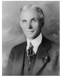
The concept of lean manufacturing has been a topic of

much discussion since Henry Ford conceived the concept

of an assembly line for the production of the Model T

Ford back in 1913.

The assembly line that was developed by Ford and his team at the Michigan

Automobile Factory was a simple one. A motor-drawn rope pulled the chassis pass a

number of workstations where workmen performed various operations resulting in a

completed automobile at the end of the assembly line.

This simple concept along with

other improvements over an 8 year

period such as, the introduction of

the conveyor belt, reduced the

assembly time of a Model T car

from 14 hours to 1 hour 33

minutes and enabled a reduction in

the selling price from $1000 in

1908 to $360 in 1916.

2.2 Line Balancing

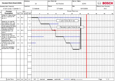
Line balancing is the assignment of operator tasks at workstations to balance

operator loops in such a way that the assembly lines output is optimized.

Figure 1: Henry Ford (1919)

Ever since the introduction of the assembly line by Henry Ford in 1913, line

balancing has been an optimization problem of significant industrial importance: the

efficiency difference between the optimal and sub-optimal assignment can yield

economies (or waste) reaching millions of dollars ( Falkenauer 2007).

The above worksheet is an example of a typical line balancing exercise. It clearly

shows that the quickest operator loop that can be achieved is determined by the

bottleneck station. In the example, the actual cycle time of the bottleneck station is

30.5 seconds and is shown as the red dashed horizontal line. If the cycle time of the

bottleneck station was to increase for any reason the output of the assembly line

would be immediately effected. Cycle time data is one of the most important items

Assembly line blancing has become a major focus in modern manufacturing

processes, the aim of which is to optimize machine and worker patterns to provide

maximum output with minimal waste.

2.3 Trends in Current Manufacturing

Manufacturing companies have 2 ways to make a profit.

1.

To increase the selling price.

2.

To reduce the cost of production.

As the selling price is generally determined by market conditions most companies

turn to reducing the cost of production to maximize profit.

To reduce the cost of production, companies aim to achieve the following goals;

Reduce Cost – By eliminating waste, anything which does not add value to

the product. This can relate to motion ( time looking and walking)

overproduction, inventory (excess stock on hand), waiting time or double

handling.

Create a flexible system that can quickly respond to change –

The Vehicle Manufacturing Industry has an ever changing working

environment due to, production levels changing with customer demands,

absenteeism changes per day and continuous improvements in the

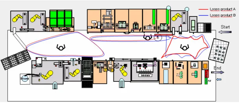
Figure 4 above shows a typical high flexibility production line designed to meet the

cost and flexibility targets set by most manufacturers. This production line consists

of 17 workstations which are shared between 3 operators and produces 2 different

product combinations.

Manufacturing companies dedicate large amounts of resources and funds to optimize

work place layouts and increase worker efficiency.

This optimization process is based on workstations performing their expected

functions within a predetermined cycle time. Any deviation from the expected cycle

time will have a large impact on the assembly line output.

The simple example below shows what effect a variation of 1 second in one worker

loop can have on the lines output.

Assuming the line has a cycle time of 30 seconds and all loops have a balanced

operator loading. Under normal conditions 120 parts would be produced in one hour.

If the bottle neck station in loop 3 has an increase in its cycle time by 1 second the

As all 3 loops would be affected by the increase in cycle time, worker efficiency and

utilization are also reduced by 3%.

This reduction in output is a perfect example of MUDA (waste) according to TPS

(Toyota Production Systems).

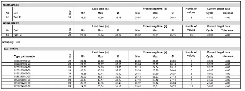
2.4 Current Cycle Time Data

The cycle time data provided by most manufacturing information system is usually

an average value over a certain period of time per product type as shown in the

Figure 5 below.

The data provided in such reports is historical in nature and not sufficient for a real

time analysis of an equipments performance. Additionally the data provided is

insufficient to enable analysis of sub cycles of the equipment. The processing time in

the above statistics varies from a minimum of 22.19 seconds to a maximum of 26.77

seconds for the part number 0265231xxx product family, a variation of 4.58 seconds.

Analysis of equipment sub-cycles is not possible from the currently available data

2.5 Real Time Data via OPC

In recent years automation technology has developed to a level that allows seamless

exchange of information across plant and enterprise networks, (Shimanuki 1999)

allowing access to real time data from Automation devices.

OPC stands for

OLE for

Process

Control (Matrikon 2005). OPC is one of the

technologies that allows the exchange of data between automation devices and it

significantly reduces the time, cost and effort required to write custom interfaces to

different intelligent devices in use today. OPC provides a standard scalable way to

collect and archive critical IT asset data and deliver it to decision makers so that it

can be acted on in a timely manner (Murphy 2006).

OPC Data Access or OPC – DA is the OPC specification that is used to read and

write real time data exclusively (Kondor 2007). It is a published specification that is

being adopted by an increasing number of manufacturers in the automation industry.

It sets out how data should be structured and allows devices from different vendors

to communicate. OPC is based on Microsoft’s COM and DCOM technologies. The

OPC foundation, a non-profit international organization made up of hardware and

software companies, is responsible for establishing and maintaining the

specifications. The specification states that each data point shall include three

attributes: a value, a quality and a time stamp. The time stamp reflects the time at

which the server knew the corresponding value was accurate (OPC Interface

OPC performance is more than adequate for most dedicated and distributed

applications running on commonly available hardware (Liu, J 2005). Studies have

reported OPC servers supplying 20,000 values per second to 4 clients with only 10

percent CPU load. (Chisholm, A, 1998)

2.6 TPM and Predictive Maintenance

Total Productive Maintenance (TPM) is a maintenance philosophy that is associated

with the lean manufacturing model (Carreira 2004). Lean production models are

based on reducing work in progress (WIP) which requires a balance of operations,

continuous material flow and minimal variation; some would call this predictability

(Carreira 2004). Predictability would imply that equipment cycle time is stable and

consistent over a extended period of time.

As maintenance departments move towards a predictive maintenance strategy,

accurate and timely information on the state of assets can be used to detect and

correct impending problems before they become catastrophic failures.

The ISO/TS 16949 defines predictive maintenance as: activities based on process

data aimed at the avoidance of maintenance problems by the prediction of likely

failure modes.

Section 7.5.1.4 “Preventive and predictive maintenance stipulates that the

organization

shall

utilize predictive maintenance methods to continually

improve the effectiveness and efficiency of production equipment”.

The aim of any data collection exercise is to get the right data, to the right people, at

2.7 Benchmarking

Benchmarking is the process of determining who is the very best, who sets the

standard, and what that standard is (Reh 2007).

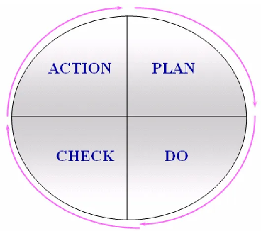
Benchmarking is another tool which is used by organizations to improve their quality

and or output. It follows a similar approach to the PDCA (Plan Do Check Act)

continuous improvement cycle.

The steps involved in a benchmarking project are:

1.

Determine who is the Best. (Plan)

2.

Determine how good they are. (Do)

3.

How do we get that good. (Check)

Any cycle time reduction project can also be considered a benchmarking activity

with the following steps.

1.

Determine the optimum cycle time. (Plan)

2.

Design processes and workflow to optimize cycle time. (Do)

3.

Continually monitor cycle time. (Check)

4.

Implement improvements based cycle time results. (Act)

Step 3 of the above project requires some form of continual monitoring so that the

cycle time achieved by the project is maintained. This is an Ideal application for

some form of cycle time analyser.

Equipment processing time (cycle time) or sometimes referred to as

throughput

is a

major factor that can effect the output of an assembly line. Equipment cycle time

remains largely unchecked in a lot of manufacturing organizations and can have

variations of up to a couple of seconds before the effects are noticed as a reduction

in output. Each year companies spend large amounts of money to improve and

increase the productivity of their equipment but spend little to monitor and

“benchmark” their gains.

2.8 Summary

History has shown that manufacturing organizations are continually working to

improve assembly line quality and output. Line balancing, TPM, Predictive

maintenance and benchmarking are some of the methods used to achieve

Once improvements have been made some form of monitoring should be

implemented to ensure that the gains achieved are maintained well into the future.

An equipment cycle time analyser would provide a means to monitor improvements

that have had a positive effect on equipment cycle time.

An equipment cycle time analyser should be capable of recording the overall and sub

- cycle processing times from automated assembly equipment and report any

deviations to the user. This data can then be used to investigate the cause of the error

Chapter 3 Methodology

3.1 Overview

A number of key elements need to be addressed in the design of the cycle time

analyser software. These elements are:

1.

Design process model

2.

Communication with OPC server

3.

Development of user interface

4.

Design and implementation of reports

5.

Programming language selection

6.

Analysis of cycle times

The Methodology adopted for these elements are discussed in this chapter.

3.2 Design Process Model

Due to the tight timelines and need for concurrent development, required by this

project, a RAD (Rapid Application Development) model was chosen for the project.

The RAD model allows for concurrent modelling, development and construction

phases to occur during the life cycle of the project.

The Development activities will be split into the following concurrent tasks:

1.

Communication with OPC server

2.

Development of User interface

3.

Design and implementation of reports

3.3 Communication with OPC Server

This task involves the investigation and set up of client and server devices to enable

the exchange of OPC data using existing Ethernet infrastructure.

The existing network structure has been designed to operate sensible control systems

and test equipment for real time measurements without any interference or

disturbance coming from local area networks and other data traffic. The system is

implemented with a separate VLAN / subnet utilising a dedicated 3 layer switch.

This provides a better split in subnets and a more secure separation from the

core-layer 3 switches of the network. Figure 7 is an example of an access control list

entry.

Figure 7: Typical “ACL” Entry

The production network is also protected with access control lists to limit incoming

and outgoing traffic only to authorised users.

3.4 Development of User Interface

The user interface to be provided should be easy to use. The choice of programming

language to be used for the project was also based on the need for a graphical user

interface. The user interface should provide an intuitive means to connect and

monitoring points to the application. Results should be displayed as a numerical

value in addition to a go, no-go indication.

3.5 Design and Implementation of Reports

To be able to analyse the results collected during the monitoring process some

method is required to visualise and compare the results obtained. As Microsoft Excel

has extensive built in functions to display graphs and manipulate the associated data,

it was decided that the implementation of the cycle time analyser should incorporate

an excel component for reporting. The reporting function must have the ability to

display all 16 recorded signals on one graph so the relationship between the signals

can be identified. Additionally there should be the possibility to overlay a reference

curve over the last recorded curve so that variations in signal times can be compared.

Excel’s standard functionality will provide useful functions such as the ability to

zoom into a section of the chart by changing the axis scale.

3.6 Programming Language Selection

Visual Basic was selected for the software implementation of this project. This

language was chosen due to the large amount of supporting documentation and

programming examples identified during the literature review. Numerous examples

and a wide selection of reference material is available to assist in the development of

a software program with respect to OPC connectivity. Additionally the OPC

foundation provides an Automation wrapper DLL suitable for use with Visual Basic.

Visual Basic also provides an efficient environment for developing software

3.7 Analysis of Cycle Times

3.7.1 Machine Capability

A machine capability study refers to a short term study with the sole aim of

discovering the machine specific effects on the production process. These principles

can be extended to determine the allowable limits that should be applied to the

recorded values of cycle time to ensure stable monitoring results.

The aim of a machine capability study is to reach a conclusion about the behaviour of

machine (in control or not?). The following formula is used for the calculation of

capability.

\

6

m

s

T

C

•

=

Where

C

= Capability index

T = Tolerance = USL-LSL

s

= total standard deviation

The capability formula above can be transformed to derive the allowable tolerance

times based on a required capability index,

total

m

s

C

T

=

•

6

•

The Tolerance value needs to be divided by 2 as the cycle time analyser uses a +/-

tolerance value.

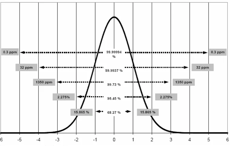
Figure 8 shows the relationship between a calculated Cmk value and a fraction

nonconforming, a Cmk = 1.33 corresponds to 32ppm non-conforming and a Cmk =

Figure 8: Normal Distribution

3.7.2 Simplified Machine Capability

As capability studies can be very time consuming when considering the large number

of values to record, a simplified approach can be adopted to derive tolerance times.

Using this approach a reduced number of samples can be used to calculate tolerance

times provided a capability index of 2 is applied.

If this approach is used the resulting tolerance time should be subject to a reality

check to confirm it’s suitability to detecting variations in cycle time.

The simplified approach should only be used on sub cycles with minimal variation

otherwise the assumed capability of 2 will result in unrealistically large tolerance

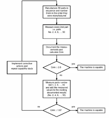
The simplified approach is based on the flow chart shown in Figure 9.

Figure 9: Machine capability process flow

3.7.2 Example Tolerance Calculation.

Table 1 contains 50 Samples taken for a machine press movement.

1 2 3 4 5 6 7 8 9 10

Calculated s

= 0.058

Now, T =

C

6

S

= 1.67 6 0.058 = 0.58

This value describes the total tolerance and needs to be divided by 2 to specify an

upper and lower limit values.

Tolerance = 0.58 / 2 = 0.29 seconds

In this example 0.29 seconds should be entered into the tolerance field and the

average of the 50 measurements, 2.351 seconds should be entered as the base value.

3.8 Chapter Summary

The main issues in the design of the cycle time analyser system will be addressed by

the selection of programming language and appropriate communication to provided a

cost effective and functional application. Issues that arise due to unforseen

circumstances will need to be reviewed as they occur and appropriate actions put in

Chapter 4 System Development and Implementation

4.1 Overall Description

The development and implementation of the cycle time analyser application involved

the following main activities:

Connection of the equipments OPC server to Visual Basic client application.

DCOM settings to allow data exchange between server and client.

Programming of client software application.

These activities and associated tasks are discussed in this chapter.

4.2 OPC Communication

OPC is a standardised interface that allows access to process data. It is based on

Microsoft’s COM/DCOM which has been extended to meet the needs of data access

in the automation process where it is mostly used to read and write data from

computer based control systems. Typical OPC clients are visualisations and

programs for recording operational data.

Due to the features of DCOM it is possible to gain access to an OPC server that is

installed on a remote PC. Another advantage of the adoption of COM technology by

OPC is programming language independence.

OPC was chosen as the communication medium for this project due to it’s ability to

support multiple clients and it’s focus on providing process data to client programs.

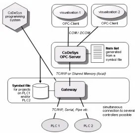
Figure 10 shows the system architecture for typical OPC systems highlighting the

Figure 10: Architecture of the CoDeSys OPC server

4.3 OPC OPCDAAUTO.DLL

A common way is needed for automation applications to access data from field

devices or databases. The OPC Data Access Automation defines a standard way by

which automation applications can access process data.

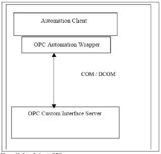
Figure 11 shows an OPC client utilising the “wrapper” DLL to call into an OPC

Server. The wrapper translates between the custom interface provided by the server

Figure 11: Interfacing to OPC servers

The OPC foundation provides a sample of the Data Access Automation interface for

the foundation members use in providing an Automation interface to OPC data

access custom interfaces. The sample provided has been used in the implementation

of this client application.

4.4 User Permission Considerations

To allow communication between two computers each machine needs to be set up so

that they have permission to access each other. This is a two way street. The client

must have permissions to access the machine with the OPC server and visa versa. If

you do not have permissions set to allow communication in both ways, then all

attempts to establish communication will be unsuccessful. For the purposes of this

project user permissions for DCOM have been opened up to allow access to all users.

established and testing completed that user permissions should be reviewed to only

allow the necessary users access.

4.5 DCOM Setting Required

See Appendix C for necessary DCOM settings.

4.6 Recording Format

The cycle time application allows for 16 discrete signals to be monitored.

Each signal is sampled at a 50ms interval with a set number of 670 samples per

signal. This resolution will allow for an overall equipment cycle time of

approximately 33.5 seconds to be recorded. The individual samples are temporarily

stored an array as shown in Figure 12 before being transferred to a text file in a tab

delimited format.

Figure 12: Visual Basic data array

The text file is used to upload the recorded data into Microsoft Excel for the

Figure 13 shows the format used for the tab delimited text file.

Figure 13: Text file format

4.7 Operation of Cycle Time Analyser Software

Figure 14 shows the main screen developed for the cycle time analyser application.

It consists of a number of sections:

1.

Connection to OPC server

2.

Create OPC Group

3.

Add OPC items to group

4.

Start recording

5.

Cycle time display

These sections are described in more detail below.

4.7.1 Connection to OPC Server

The first step in the operation of the cycle time analyser software is to establish

connection to the selected automation controller and select the required OPC server.

This is achieved by entering the required node name (IP address or computer name)

and then pressing the “List OPC Servers” button. A list of available OPC servers will

then be displayed. Select the required OPC server and click the “Connect button”

Once Connection to the OPC server has been established the “Add group” button

will become active. Figure 15 shows the server connect section of the cycle time

analyser application.

4.7.2 Create OPC group

Type the name of the OPC group to be added and click the “Add Group” button.

Figure 16 shows the Add Group to OPC Server section.

Figure 16: Group connect

4.7.3 Add OPC Items to Group

OPC items can now be added, these represent the input, output or internal memory

locations that should be monitored. These can be typed directly into the 16 fields

provided or uploaded from a text file using the “Load I/O” button.

Appendix B shows an extract from the target equipments OPC variables list. OPC

items need to be entered in the item fields using the same naming convention as

displayed in this extract.

Trigger points can also be selected:

Trigger - determines the signal which will start the recording process,

positive edge trigger.

End - determines which signal is to be used to calculate the overall

Figure 17 shows the OPC Items section.

Figure 17: Add Items

4.7.4 Start Recording

After connection is established and OPC items have been added, the start recording

button can be pressed to begin the recording process. When the signal marked with

the ‘Trigger’ changes to a high state recording will begin.

Once recording has finished indicated by the progress bar the fields Start, End and

Seconds will contain data from the recording process.

Start – Time of Trigger. (start Trigger)

End – Time of end signal.

Figure 18 shows the function buttons.

Figure 18: Function buttons

4.7.5 Cycle Time Display

Additionally at the end of recording all signals that have undergone a low – high -

low transition will have their sub-cycle times presented in Cycle times section of the

display as shown in Figure 19.

Figure 19: Results display

Times that are displayed in green represent times that fall within the base time +/- the

tolerance time.

Times that are shown in red and have a zero (0) value represent, times that had a high

state at the end of the recording cycle.

4.7.6 User Instructions

A comprehensive instruction manual was developed for the cycle time analyser

software which can be found in appendix C.

4.8 Testing

Testing involved a number of stages.

1.

Testing connection between client and server.

2.

Verifying data recording.

3.

Report

The first stage was to test the OPC connection and establish that the required

information could be accessed by the Visual Basic client program. Initially an

attempt was made to establish communication using the corporate network. This

involved a number of challenges due to the existing network configuration. With the

mixture of domains, workgroups, password rules, access control lists and different

subnets, standard DCOM settings could not be adopted to allow communication

between the client and server computers. An alternative solution is discussed in

section 4.11.2 but as this was not the main focus of this project it was decided to use

a computer connected to the same subnet and using the same username / password

combination as the server computer for testing purposes.

The next stage of testing involved running the cycle time analyser application and

performed on a piece of equipment that had no moving components to reduce the

risk of equipment damage that may have occurred from potential software issues.

The test was performed initially by changing the machine operating mode from

automatic to manual and recording the associated OPC items. This test proved that

accessing the OPC server with a second client had no adverse effects on the systems

operation.

The final stage of testing involved taking a number of recordings at different cycle

times and comparing the results. A test was conducted by adjusting the robot speed

from 100% to 30% and recording the results of the overall cycle time. The results in

table 1 show the variation in overall cycle time as the robot speed was varied.

Table 2: Overall cycle time variation

4.9 Visualisation of Recorded Data

Microsoft Excel was chosen for the visualisation of the recorded data due to it’s

ability to easily manipulate and format data. Both data and reference files are stored

as tab delimited files and are read into excel using Visual Basic macro’s.

% Speed

Cycle time

Difference

100

36.511

0

75

36.719

0.208

50

38.550

1.831

Once the data is read into the respective excel sheets Data and Reference, it is

formatted to show the data for each of the 16 bits monitored as single step time traces

on a displacement diagram as shown in Figure 20.

Figure 20: Excel report

The excel report performs the following functions

•

Import data and reference files

•

Show reference

•

Input text description for signals

•

Diagram 1, format suitable for printing

4.10 Visual Basic Limitations

The interval property associated with Timer controls in Visual Basic have some

•

If an application is making heavy demands on the system such as long

loops, intensive calculations, drive, network, or port access, the cycle

time program may not receive timer events as often as the Interval

property specifies.

•

The system generates 18 clock ticks per second — so even though the

Interval property is measured in milliseconds, the true precision of an

interval is no more than one-eighteenth of a second.

Considering these limitations it is recommended that this application be run in

isolation to reduce the load on the system.

4.11 Problems Encountered

4.11.1 OPC TimeStamp

The majority of OPC servers provide Item timestamp information in UTC format

which provides a time resolution down to milliseconds. However Microsoft Visual

Basic does not provide any formatting instructions for retrieving milliseconds from

the UTC format.

After much investigation and a recommendation from the OPC Foundation Forum

the VariantTimeToSystem function was perceived as a solution to this issue.

The VariantTimeToSystemTime function was tested and was also not able to return

the millisecond component of the timestamp.

After further investigation, a Microsoft knowledge base 297463 was discovered that

supported the conclusion that the VariantTimeToSystemTime was incapable of

Finally the decision was made to write a small subroutine to calculate the millisecond

value from the timestamp. The milliseconds are then concatenated on to the

“hh:mm:ss” format to provide a timestamp with millisecond resolution

“hh:mm:ss.000”

Figure 21 shows the code used for the millisecond conversion.

Figure 21: Code for Millisecond conversion

4.11.2 DCOM Security Settings

Initially an attempt was made to connect to the OPC server from an office computer

that was a member of a domain whilst the computer with the OPC server was

situated in a workgroup. The configuration required to enable communication using

DCOM proved increasingly difficult and was abandoned as it was not the primary

' This function converts.UTC based timestamp and extracts milliseconds

‘ Calculate total milliseconds in time stamp

' Convert date time format to double

Dummy1 =

CDbl

(varDateTime)

' Remove fractional part of number

Dummy2 =

Fix

(varDateTime)

Dummy3 = varDateTime - Dummy2

Dummy3 = Dummy3 *

100000000

Dummy3 =

Int

(Dummy3)

TotalmSec = Dummy3

' Extract hours from time stamp

Hours =

Fix

(Int(Dummy3 /

3600000

))

Dummy3 = TotalmSec

' Extract Minutes from time stamp

Minutes =

Fix

(((TotalmSec - (Hours *

3600000

)) /

60000

))

Dummy3 = TotalmSec

' Extract seconds from time stamp

Seconds =

Fix

(((TotalmSec - (Hours *

3600000

) - (Minutes *

60000

)) /

1000

))

' Extract milliseconds from time stamp

Milliseconds =

Fix

((TotalmSec - (Hours *

3600000

) - (Minutes *

60000

) -

(Seconds * 1000)))

' Format time output into “00:00:00.000”

focus of this project. Other alternatives were investigated resulting in the discovery

of an OPC tunneller software from a company called Matrikon which effectively

connects OPC client and servers independent of DCOM settings. The cost of the

OPC tunneller software provided by Matrikon prohibited its use in this project, see

Appendix E. Use was made of the 30 day trial period offered by Matikon for

evaluation purposes. This software made connection to OPC servers on different

subnets remarkably easy and would be considered as a permanent solution to resolve

DCOM issues if the cycle time analyser concept is implemented.

4.11.3 SyncRead does not Return Timestamp Data as Array

The SyncRead function has two optional variables, Qualities and Timestamps.

In the OPC Data Access Automation Interface Standard these are defined as

“Variants containing a Date array of UTC time stamps for the Timestamps variable

and a Variant containing an Integer array of Qualities for the Qualities variable”.

Upon further investigation a similar query had already been posted on the OPC

foundation’s forum page on 14

March 2003, suggesting that the following special

logic be used to convert the variants to arrays before the data can be accessed.

// Convert Variant containing Date array to Array

Dim

TimeStamps()

As Doub

le

ReDim

TimeStamps(ItemCount)

If

VarType(TimeStamp) = vbArray + vbDate

Then

Dim Buffer1()

As Date

Buffer1 = TimeStamp

For

ii = 1

To

ItemCount

TimeStamps(ii) =

CDbl

(Buffer1(ii))

Next

ii

4.11.4 OPC Server Capability

The basic update rate of the OPC-Servers used for communication is specified as

milliseconds = cycle time with which all item data are read from the controller. This

data is then written into the cache with which the client communicates with a

separately defined update rate.

In comparison to direct access to the controller, reading and writing of variables via

this cache list leads to an increase in access time (max. approx. 1ms per item).

The user needs to be aware that using an OPC server with an excessive number of

items can reduce the accuracy of the information received from the server.

4.12 Chapter Summary

The Cycle Time Analyser application that has been developed is based on a

Windows based application that performs synchronous read requests from the

connected OPC server. The collected data represents the 16 OPC items entered in the

GUI and is compared to preset values entered into the base times screen and

tolerance time screens. The data recorded can be imported into an Excel spread sheet

Chapter 5 Conclusions

5.1 Achievement of Objectives

The aim of this project was to develop a software application that was capable of

monitoring equipment cycle time utilising the existing infrastructure. The system was

developed to the stage where equipment sub cycle times could be extracted from the

recorded data and compared with preset values determined by statistical analysis.

The software has proven to meet the requirements of a flexible and scalable system

suitable for implementation.

The objectives defined in Chapter 1 have been addressed and research into the

suitability of OPC and Visual Basic as components of the cycle time analyser have

proven to be effective.

The use of existing infrastructure caused a number of authorisation issues which

were solved by the use of a third party software application which allows PC

connectivity across conflicting network configurations.

The cycle time software was designed and implemented. The system allows real time

data to be recorded from equipment and stored in a local file for further analysis. A

comparison of recorded data is also performed with pre recorded limits to give an

5.2 Future Work

The evolution of the cycle time analyser software to it’s current level has proven the

underlying principles and indicated that the continuation of the development of

application would provide an effective monitoring tool. The following tasks are

currently seen as enhancements that could be added to the existing solution.

5.2.1 Statistical Evaluation of Tolerance Times

The stability of equipment cycle times is a necessary prerequisite to allow for

informed decisions to be made about equipment capability. The calculation of

stability and capability were performed by manual calculations as the timing of this

project did not allow for this function to be fully integrated into the software

application. The implementation of the following functions would greatly increase

the speed at which the software could be adapted to different equipment.

•

Record 100 samples

•

Calculate Capability index

•

Calculate lower and upper tolerance limits

5.2.2 Monitor Multiple Machines

The current application only allows for one machine to be monitored at a time. The

ability to monitor multiple equipment simultaneously would greatly increase the

usability of this application. Processor loading and communication bandwidth will

5.3 Final Summary

As a result of undertaking this project it has become clear that monitoring equipment

cycle time and comparing the values obtained with previously recorded values can be

used to determine equipment stability. The software application presented in this

project can be used as part of a lean system of operation and used to predict

equipment failures. It is anticipated that the cycle time analyser software identified in

this project will, after further development and testing, be adopted as a permanent

References

ISO/TS16949 Technical Specification, Quality Management Systems –

Particular

requirements for the application of ISO 9001:2000 for automotive production and

relevant service part organizations

Hobbs, Dennis P,

Lean Manufacturing Implementation: A Complete Execution

Manual for Any Size Manufacturer,

J. Ross Publishing

Bill Carreira, 2004,

Lean Manufacturing That Works: Powerful Tools for

Dramatically Reducing Waste and maximizing Profits,

Amacom, New York

Toyota Production System Manual, June 1992, Toyota

Murphy E, 2006 ‘Time for a health check’,

Focus: Open connectivity

, 24

December

2006.

Chisholm, A, 1998, ‘DCOM, OPC and performance issues’,

OPC Foundation white

paper

, 1998.

Liu, J, Wee Lim,K, Khuen Ho, W, Chen Tan, K, Tay, A, Srinivasan, R 2005

‘Using

the OPC Standard for Real-Time Process Monitoring and Control’,

IEEE Software

, November/December 2005, page 54.

Yoh Shimanuki, 1999, ‘OLE for Process Control (OPC) for New Industrial

Automation Systems’, IEEE

Robert Bosch gmbh

Machine and Process Capability, 3

edition 2004

Kondor, R, 2007, Matrikon, ‘Understanding OPC: Basics for New Users’

http://ethernet.industrial-networking.com/articles/article

How to cycle time

http://www.optimaldesign.com/OLHelp/HowTo/HowToCycleTime.htm

Line Balancing in the Real World, Emanuel Falkenauer, 2007 viewed on 6

May

2007.

http://optimaldsign/Download/OptiLineFalkenauerPLM05.pdf

Birth of the Assembly line, 2007 viewed on 6

May 2007.

http://autopopuli.blogspot.com/2006/10/birth-of-assembly-line.html

Wikipedia

, 2007, viewed on 6

May 2007.

http://en.wikipedia.org/wiki/Henry_Ford

Reh, J, 2007 ‘Benchmarking’, viewed on 16th May 2007,

Appendix A

Appendix B

Appendix C

RBAU

Cycle Time Analyser

OPC Cycle time analyser3.doc

RBAU/MFA1, 09/2007

System for Analysis of Cycle Time

of Production Equipment

with

OPC

RBAU

Cycle Time Analyser

OPC Cycle time analyser3.doc

RBAU/MFA1, 09/2007

1. Table of Contents

1. Table of Contents...57

2. Purpose and Aim of Cycle Time Analysis ...58

2.1.Extension of cycle time monitoring...58

3. System Configuration...59

4. Summary...59

5. Prerequisites ...59

6. Program Installation ...60

7. Network setup ...60

8. DCOM settings...60

9. Cycle Time Analyser Operation ...61

9.1 Loading Items from File...62

9.2 Connect to OPC Server ...63

9.3 Add Group to OPC Server ...64

9.4 Adding and Displaying Items...64

9.5 Start recording ...66

9.6 Cycle time results...67

9.7 Base times ...68

9.8 Tolerance times ...69

9.9 Displaying results in excel...70

9.9.1

Input sheet data ... 72

9.9.2

Zoom... 73

9.9.3

Excel Diagram 1... 74

RBAU

Cycle Time Analyser

OPC Cycle time analyser3.doc

RBAU/MFA1, 09/2007

2. Purpose and Aim of Cycle Time Analysis

Frequently the requirement exists to optimise the cycle time of existing production,

assembly or test equipment.

In the case of complex control systems, the chronological reference to the state of

sensors and other components are not directly obvious from the machine program.

Deviations from the designed cycle time are difficult to locate.

The method applied so far is to record signals using a multi-channel recorder.

This method has a number of disadvantages:

- Only possible to monitor sensors or hard signals.

- Recording of a very limited number of signals.

- Considerable effort is required to connect individual signals.

The aim is to generate an analyser diagram from the control system of the

equipment.

With this system of cycle time analysis it is possible to chronologically record all

signal changes of the selected inputs / outputs of a complete machine cycle.

The system is connected to the automation controller.

2.1. Extension of cycle time monitoring

RBAU

Cycle Time Analyser

OPC Cycle time analyser3.doc

RBAU/MFA1, 09/2007

3. System Configuration

4. Summary

Prior to recording, the machine specific inputs and outputs are allocated to items and

entered in the item allocation table. There is a facility to read the input items from a

file.

After recording, data is stored in a text file “data.text" and can be imported to the

cycle time analyser Excel sheet for visualisation and analysis.

5. Prerequisites

Microsoft Excel

Access to Equipment subnet

PC with required DCOM and network configuration.

Automation controller Industrial PC – Windows XP Existing Visualisation

Integrated in Controller

RBAU

Cycle Time Analyser

OPC Cycle time analyser3.doc

RBAU/MFA1, 09/2007

6. Program Installation

The PC program is available on disk as “OPC Cycle Time Analyser.exe” and may be

copied to any directory.

The recording sample is stored in the temp directory on C drive: “C:\temp\data.text

A reference sample can also be saved on C drive “C:\temp\ref.

7. Network setup

This section describes how to adapt the network configuration to allow your PC to

connect using TCPIP with the equipment to be analyzed.

-

Change DCOM settings on your PC and equipment to those recommended in

section 8

-

Connect your PC to same subnet as the installed equipment.

-

Change your IP address to one that is located in the same subnet as your

equipment

-

Create a user with the same login details “user name and password” as the target

equipment.

-

Map a network drive to the target equipment to be monitored.

8. DCOM settings

RBAU

Cycle Time Analyser

OPC Cycle time analyser3.doc

RBAU/MFA1, 09/2007

9. Cycle Time Analyser Operation

OPC Server Connection: Connection is established to required OPC server by listing all servers available and selecting required server

OPC Group:

Enter name of OPC server group.

Function Buttons: Operator button for starting , loading Items and saving reference diagram.

Screens:

These buttons open the cycle times, Tolerance and base values screens

OPC Items:

16 items can be monitored by the OPC Analyser and are entered into these fields. Alternatively Items can be loaded from a pre written text file with the Load I/O function.

Cycle times:

Measured cycle times are displayed after the measurement time is complete.

Triggers:

RBAU

Cycle Time Analyser

OPC Cycle time analyser3.doc

RBAU/MFA1, 09/2007

9.1. Loading Items from File

The list of OPC Items to be monitored can also be loaded from a text file. This makes

the adaptation for another machine much quicker than entering individual items.

The file must contain the proper OPC item descriptions, similar to those in the

example below.

Enter a maximum of 16 items to be copies to

OPC Items.

This file can be created in a text editor like

Notepad or Ultraedit.

Click on the Load I/O to open the I/O text file

RBAU

Cycle Time Analyser

OPC Cycle time analyser3.doc

RBAU/MFA1, 09/2007

OPC Items are now copied from the I/O file to the OPC Items in the cycle time

analyser screen.

9.2. Connect to OPC Server

This section describes how to list and connect to an OPC server:

-

Input Node Name IP address

-

Click

List OPC Servers

-

Select the required OPC server

-

Click

Connect

Enter the IP address of the equipment that has the OPC server you wish to connect to. If no IP address is entered OPC servers on the local machine will be listed.

Click “List OPC Servers after you have entered the IP address. A list of available OPC servers will be displayed.

RBAU

Cycle Time Analyser

OPC Cycle time analyser3.doc

RBAU/MFA1, 09/2007

9.3. Add Group to OPC Server

This section describes how to add a group to the OPC server

-

Type the Group Name

-

Click

Add Group

9.4. Adding and Displaying Items

This section describes how to add OPC items.

-

Type the OPC Items or load OPC Items as described in Section 9.1.

-

Select the required Trigger and End signals.

RBAU

Cycle Time Analyser

OPC Cycle time analyser3.doc

RBAU/MFA1, 09/2007

Enter the required OPC Items required to be monitored.

Note: Names used here must match those loaded into OPC server.

Select the required trigger points.

Trigger – on the low to high transition of this signal recording of time stamp values will commence.

End – the low to high transition of this signal will be used to determined the overall cycle time

Click Add OPC Items to add entered items to OPC server.

Value:

During recording the actual Value received for this Item from the OPC server is shown here.

Time Stamp:

RBAU

Cycle Time Analyser

OPC Cycle time analyser3.doc

RBAU/MFA1, 09/2007

9.5. Start recording

This section describes how the analyzer is started and some other related functions.

-

Click start recording button.

-

Time stamp values should now be changing as items are read from the server

-

Once the selected trigger item has a 0 to 1 transition the recording progress bar

will be active.

-

The progress bar will show when the recording process is finished.

-

Once recording is finished the fields Start, End and Seconds will display values:

Start - is the time the trigger 0 to 1 transition.

End is the time of the end trigger 0 to 1 transition

Seconds is the calculated difference

Progress bar, shows recording process starts when trigger activated.

Start displays the value of

the start trigger. End displays the value of the end trigger after recording.

Seconds the time difference between trigger start and trigger end signals. Start recording – starts real

RBAU

Cycle Time Analyser

OPC Cycle time analyser3.doc

RBAU/MFA1, 09/2007

9.6. Cycle time results

This section shows the Cycle times results screen.

-

Items highlighted in green identify items within the tolerance time.

-

Items highlighted in red identify items outside the tolerance time.

RBAU

Cycle Time Analyser

OPC Cycle time analyser3.doc

RBAU/MFA1, 09/2007

9.7. Base times

This section shows the Base times screen.

RBAU

Cycle Time Analyser

OPC Cycle time analyser3.doc

RBAU/MFA1, 09/2007

9.8. Tolerance times

This section describes the Tolerances screen.

-

Tolerance times obtained by statistical analysis of process cycles are entered on

this screen.