Modified Richards equation and its exact solutions for soil water dynamics on eroding hillslopes

Modified Richards equation and its exact solutions for soil water

dynamics on eroding hillslopes

Ninghu Su

School of Mathematical Sciences, Queensland University of Technology, Gardens Points Campus, Brisbane, Queensland, Australia

Received 24 May 2000; revised 5 February 2002; accepted 22 February 2002; published 12 June 2002.

[1] The modified Richards equation (MRE) is presented by using a rotated coordinate system to accommodate the geometry of a hillslope and a moving boundary to represent an eroding surface on a hillslope. Exact analytical solutions of MRE are developed subject toFujita’s [1952] diffusivity and Sander et al.’s [1988] unsaturated hydraulic

conductivity. The mathematical analysis presented here for soil water dynamics and infiltration in particular on an eroding hillslope deviates from the traditional way in which infiltration has been investigated sinceGreen and Ampt’s [1911] pioneering work. The MRE clearly improves mathematical representation of physical reality. Field data are used to derive parameters in a solution of MRE to illustrate the effect of erosion rates on soil moisture profiles in a moving boundary. INDEXTERMS:1655 Global Change: Water cycles (1836); 1815 Hydrology: Erosion and sedimentation; 1866 Hydrology: Soil moisture; 3210 Mathematical Geophysics: Modeling;KEYWORDS:modified Richards equation, erosion, soil water flow

1. Introduction

[2] Numerous studies have been reported on quantifying

soil water movement and infiltration sinceGreen and Ampt

[1911] proposed the first infiltration model. These studies regard the infiltration surface as a stable surface on which infiltration takes place, which is reasonable only for infil-tration on flat surfaces. On a slope, however, runoff formed during rainfall erodes and entrains soil particles and solutes from the slope surface and moves them downslope, and soil erosion processes remove some of the topsoil, thus forming a new surface for the same processes to be repeated. In this case, the traditional infiltration theories do not apply.

[3] In this paper, we investigate soil water dynamics on a

dynamic eroding hillslope which implies that two more concepts are introduced: one is a dynamic eroding hill-slope, and the other is soil water movement on the dynamic slope. With these two concepts developed for soil water dynamics on eroding hillslopes, it is clear that the method-ologies proposed in this presentation are more realistic and more reasonably represent natural hydraulic phenomena and improve mathematical representation of the physical processes.

2. Richards Equation for Soil Water Physics on an Eroding Hillslope

[4] Starting from Buckingham’s concept of potentials, a

nonlinear Fokker-Planck equation became the law for the study of flow in unsaturated soils since Richards [1931], which can be written [Philip, 1991]

@q

@t¼ r ðDðqÞrqÞ dK

dq

@q

@z; ð1Þ

where

q the soil moisture content;

D(q) the diffusion coefficient;

K the hydraulic conductivity;

z the depth of soil;

t time;

r Laplacian operator.

[5] Equation (1) has been extensively investigated in

soil physics and related areas in the last seven decades since Richards[1931] and has been used for modeling soil water movement including infiltration subject to different conditions.

[6] As far as infiltration is concerned, it is obvious from the

literature that the vast majority of mathematical formulations and related various solutions published so far were developed for infiltration on a flat surface only. Various solutions for infiltration subject to different boundary conditions and different forms of the diffusion coefficient and hydraulic conductivity have been developed. For a limited number of reviews on this topic the reader is referred toPhilip[1969, 1991],Parlange et al.[1980], andSposito[1995].

[7] In order to incorporate the effect of hillslope in

Richards equation for infiltration, Philip [1991] presented a modified Richards equation and related solutions for infiltration on planar slopes. However, Philip’s approach is applicable to stable slopes only. As hillslopes are often susceptible to erosion, infiltration and related processes cannot be correctly interpreted using Philip’s approach when erosion occurs.

[8] In this paper, we present procedures for analyzing soil

water relationships on eroding hillslopes. These method-ologies and procedures are based on the Richards equation and are linked to soil erosion processes.

[9] In order to clarify the definition to be used in this

paper, Figure 1 draws a schematic illustration of the definitions used in the analysis. Figure 1 also highlights Copyright 2002 by the American Geophysical Union.

0043-1397/02/2001WR000373$09.00

the key points of departure from the traditional theories on soil erosion and soil water flow.

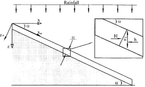
[10] In Figure 1, the following nomenclature is defined.H

is the depth of soil layer to be eroded during a rainfall event;

his the vertical depth of the same soil layer inclined at an angle of a; and x and z define the Cartesian coordinate, which after a rotation by an angle ofa, is defined by (x*,z*).

[11] In Figure 1 the relationship betweenHandhis given

by

H¼hcosa ð2Þ

Figure 1 is a combination of the definitions developed in this paper and the schematic illustration of Philip [1991, Figure 1]. Figure 1 of this paper and Figure 1 of Philip

[1991] are similar in geometry except for a moving boundary used in the present paper.

[12] With the aid of Figure 1 in this paper the

coor-dinates (x_*, z_{*) rotated by an angle of} a are given by

Philip [1991],

x_*¼xcosaþzsina ð3Þ

z_*¼ xsinaþzcosa: ð4Þ

[13] With equations (3) and (4), equation (1) is

trans-formed to

@q

@t¼ @ @z_* Dð Þq

@q

@z_*

dK

dq

@q

@x_*sinaþ @q

@z_* cosa

: ð5Þ

[14] Philip [1991] argued that the relevant solution of

equation (5) is essentially independent ofx*, and dependent only on z* and t. In these circumstances, with the aid of

equations (3) and (4), equation (5) reduces to

@q

@t¼ @ @z_* DðqÞ

@q

@z_*

dK

dq

@q

@z_* cosa: ð6Þ

[15] Philip[1991] presented solutions of equation (6) for

hillslope infiltration and related various flow components for planar slopes. His formulations and solutions are appli-cable only for hillslope infiltration on a stable surface without material loss from the surface.

[16] In the following sections, we investigate soil

mois-ture and hillslope infiltration on an eroding surface subject to the following initial and boundary conditions:

q¼0 z_*>0 t¼0 ð7Þ

q¼qS z_*>0 t>0 ð8Þ

where qsis the saturated soil water content at the surface.

3. Analytical Solution for Soil Moisture Status on an Eroding Hillslope

[17] For analyzing water movement within and on an

eroding hillslope we introduce the average surface soil erosion rateS,

S¼H=T ð9Þ

From equation (2) we have

S¼ðhcosaÞ=T: ð10Þ

Now we have introduced two expressions forS. If the depth of soil eroded in a storm is very small, one could approximately regardHandhas equal.

[18] We further use a moving coordinate system with a

new variablex. If time is measured from the start of rainfall and runoff and soil erosion startt0after rainfall starts, then

we have

x¼z_*S tð t0Þ; ð11Þ

wheret0is the time to ponding. Equation (11) implies that at

the erosion rateSafter each rainfall event, a new soil surface forms with its origin starting at x.

[19] With the aid of equation (11), equation (6) can be

rewritten as

@q

@x¼

1 S

@ @x DðqÞ

@q

@x

þdKðqÞ

dq

@q

@x

cosa

S : ð12Þ

[image:2.594.178.413.64.205.2]

geometries and for both stable and eroding surfaces. Obviously, the MRE reduces to different forms subject to different conditions.

[20] In the present investigation, equation (12) can be

written as an ordinary differential equation,

dq

dx¼

1 S

d dx DðqÞ

dq

dx

þdKðqÞ

dx

cosa

S ; ð13Þ

and the initial and boundary conditions equations (7) and (8) now become

q¼0 x>0 ð14Þ

q¼qS x¼0 ð15Þ

A first integral of equation (13) with respect toxis

q¼ DðqÞ

S dq

dxþKðqÞ

cosa

S þC1; ð16Þ

whereC1is a constant of integration.

[21] It is obvious that the form of solutions of equation

(16) depends on the forms ofD(q) andK(q). In the rest of the section, we further investigate the solutions of equation (16) subject to one set of functions for the unsaturated hydraulic conductivity and diffusivity.

[22] We useSander et al.’s [1988] unsaturated hydraulic

conductivity,

KðqÞ ¼K1þK2qþK3q

2

1nq ð17Þ

andFujita’s [1952] diffusivity

DðqÞ ¼ D0

1nq

ð Þ2; ð18Þ

whereK1,K2,K3,D0, andnare constants determined from soil properties.

[23] Equations (17) and (18) were used by Sander et al.

[1988] to derive exact solutions of the nonlinear Richards equation for constant flux infiltration (a boundary condition of the third type). In this paper, we use equations (17) and (18) for K(q) and D(q), respectively, in equation (16) to derive a set of exact analytical solutions for infiltration on an eroding hillslope subject to the concentration boundary condition (a boundary condition of the first type).

[24] In equations (16) and (17), if we define K1= 0 for

q= 0 and dq/dx|q=0 = 0, we haveC1 = 0 forq = 0. Then,

substitution of equations (17) and (18) into equation (16) gives

dq

dxþ

1 D0

SK2cosa

ð Þqþ 1

D0

K2nK3

ð Þcosa2nS

½ q2

þ 1

D0

Sv2þnK3cosa

q3_¼

0: ð19Þ

Equation (19) can be solved analytically. First, we rewrite equation (19) as

dq

dx¼qR; ð20Þ

where

R¼AþBqþCq2 ð21Þ

with

A¼ 1

D0

K2cosaS

ð Þ ð22Þ

B¼ 1

D0

K3K2n

ð Þcosaþ2nS

½ ; ð23Þ

C¼ 1

D0

Sn2_nK 3cosa

: ð24Þ

Then we integrate equation (20),

Z dq

Rq¼

Z

dxþC2; ð25Þ

where C2is a constant of integration.

[25] Following Gradshteyn and Ryzhik [1994, equations

(2.177-1) and (2.172), pp. 81, 83], equation (25) is inte-grated to give

1 2Aln q2 R B 2A 1 ffiffiffiffiffiffiffiffi p ln ffiffiffiffiffiffiffiffi p

ðBþ2CqÞ

ffiffiffiffiffiffiffiffi

p

þðBþ2CqÞ

" #

¼xþC2;

ð26Þ

where

¼4ACB2: ð27Þ

Equation (26) takes three different forms depending on the values of [Gradshteyn and Ryzhik, 1994, equation (2.177), p. 83].

[26] Case 1 is for< 0. In this case, equation (26) gives

1 2Aln

q2

R þ B ApffiffiffiffiffiffiffiffiArth

Bþ2Cq

ffiffiffiffiffiffiffiffi

p

¼xþC2 <0; ð28Þ

where Arth Bþ2Cq1= ffiffiffiffiffiffiffiffi

p

is the inverse hyperbolic tangent function. Applying the boundary condition to equation (28) yields

C2¼ 1 2Aln

q2s

AþBqsþCq2s !

þ B

ApffiffiffiffiffiffiffiffiArth

Bþ2Cqs ffiffiffiffiffiffiffiffi

p

: ð29Þ

Substitution of (29) in (28) gives

x¼ 1

2Aln

q2 q2 s !

AþBqsþCq2s

AþBqþCq2

" #

þ B

Apffiffiffiffiffiffiffiffi

Arth Bþffiffiffiffiffiffiffiffi2Cq

p

Arth Bþffiffiffiffiffiffiffiffi2Cqs

p

<0; ð30Þ

moisture content q, erosion rate S, and other parameters incorporated in A, B, C, and . With equation (11), equation (30) can be written for the fixed coordinate systems,

z

*¼S tð t0Þ þ 1 2Aln

q2 q2s !

AþBqsþCq2s

AþBqþCq2

" #

þ B

Apffiffiffiffiffiffiffiffi

Arth Bþffiffiffiffiffiffiffiffi2Cq

p

Arth Bþffiffiffiffiffiffiffiffi2Cqs

p

<0: ð31Þ

[27] Case 2 is for= 0. In this case, equation (26) gives

1 2Aln

q2

R þ B

A Bð þ2CqÞ¼xþC2 ¼0; ð32Þ

and applying the boundary condition yields

C2¼ 1 2Aln

q2_s

AþBqsþCq2s !

þ B

A Bð þ2CqsÞ

; ð33Þ

and substitution of equation (33) in equation (32) gives

x¼ 1

2Aln

q2

q2_s

!

AþBqsþCq2s

AþBqþCq2

" #

þB

A 1 Bþ2Cq

ð Þ

1 Bþ2Cqs

ð Þ

¼0 ð34Þ

for a moving coordinate system, or with equations (11) and (34), we have

z_*¼Sðtt0Þ þ 1 2Aln

q2

q2_s

!

AþBqsþCq2s

AþBqþCq2

" #

þB

A 1 Bþ2Cq

ð Þ

1 Bþ2Cqs

ð Þ

¼0 ð35Þ

[image:4.594.51.286.65.211.2]

for a fixed coordinate system. Figure 2. Sander et al.’s [1988] unsaturated hydraulic

conductivity as a function of moisture content.

Figure 3. Fujita’s [1952] diffusivity as a function of moisture content.

[image:4.594.49.542.290.728.2]

[28] Case 3 is for> 0. In this case, equation (26) gives

1 2Aln

q2

R B Apffiffiffiffiarctg

Bþ2Cq

ffiffiffiffi

p

¼xþC2 >0: ð36Þ

Applying the boundary condition yields

C2¼ 1 2Aln

q2 1 AþBqsþCq2s

!

B

Apffiffiffiffiarctg

Bþ2Cqs ffiffiffiffi

p

ð37Þ

Substitution of equation (37) in equation (36) gives

x¼ 1

2Aln

q2 q2s !

AþBqsþCq2s

AþBqþCq2

" #

B

Apffiffiffiffi arctg

Bþ2Cq

ffiffiffiffi

p

arctg Bþ2Cffiffiffiffiqs

p

>0 ð38Þ

for a moving coordinate system, or with equations (11) and (38) we have

z_*¼S tð t0Þ þ 1 2Aln

q2 q2_s

!

AþBqsþCq2s

AþBqþCq2

" #

B

Apffiffiffiffi arctg

Bþ2Cq

ffiffiffiffi

p

arctg Bþ2Cffiffiffiffiqs

p

>0 ð39Þ

for a fixed coordinate system.

[29] The analytical solutions of the generalized Richards

equation presented above are subject to the first type boundary condition (or concentration boundary condition). With the diffusivity and unsaturated hydraulic conductivity functions described by Fujita’s [1952] and Sander et al.’s [1988] functions, respectively, these solutions given in both moving and fixed coordinate systems describe the relation-ships among soil moisture and other physical parameters on an eroding hillslope.

4. Illustrative Examples

[30] Now we illustrate the analytical solutions with data

from the field (C. H. Roth, personal communication, 2000). The details of the data used in the analysis are given byRoth et al.[1995].

[31] The data on volumetric moisture content,q(%), and

hydraulic conductivity,K(mm/hr) are used to determine the parameters in the hydraulic conductivity function in equa-tion (17). Then diffusivity, as defined by

Dð Þ ¼q Kð Þqdy=dq ð40Þ

is computed on the basis of data for the moisture potentialy

(mm) and content q(%).

[32] When the data on q andK(q) are fitted to equation

(17), the parameters appearing in the expression are derived, namely, K1 = 0, K2 = 0.1158, K3 = 0.5424, and v =

2.93744. OnceD(q) is computed using equation (40), fitting the data to equation (18) gives the values forD0= 55.8290

andv= 2.73725. The results are shown in Figures 2 and 3. [33] It should be noted that the two curves fitted

auto-matically using a computer program shown in Figures 2 and 3 have different values ofv. In the subsequent simulations presented in Figures 4 and 5, an average value ofv= 2.855 is used.

[34] With this set of parameters, it is found that< 0 in

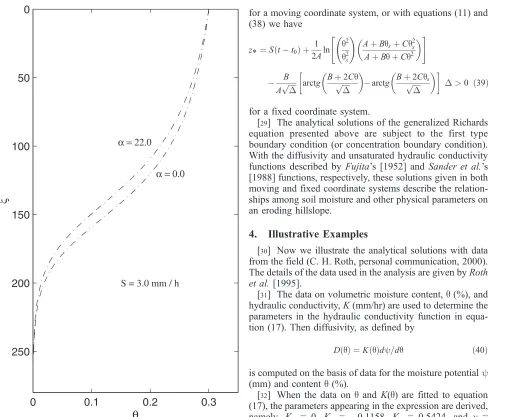
equation (27), thereby by making equations (30) and (31) applicable to this soil. Equation (30) is used to generate Figures 4 and 5 to illustrate the effects of erosion rate and slope on moisture distribution in the soil profile during simulated storm events.

[35] The curves with different erosion rates S (mm/hr)

and slopes a (degrees) are moisture profiles below the moving surface in the moving coordinatex(mm). In other words, thexversusqrelationship defines the distribution of soil moisture content below the moving surface for different erosion rates and a given slope.

5. Discussion

[36] In the preceding analysis, we have presented the

[image:5.594.58.565.56.473.2]

modified Richards equation (MRE), exact solutions of the Figure 5. Effect of slope on moisture profiles in a soil on

MRE for water movement on an eroding hillslope, and an example illustrating these solutions applied to a real soil. The following issues have been addressed in the presenta-tion

1. The analysis presented in this paper establishes a realistic model for soil moisture physics on an eroding hillslope. With the aid of a transformation into a rotated coordinate and by introducing a new variable, x, the Richards equation, which is a nonlinear Fokker-Planck equation, reduces to an ordinary differential equation. The MRE generalizes the partial differential equation governing soil water dynamics on both sloping and flat geometries and for both stable and eroding surfaces. The following is a summary of the different forms of MREs: (1) a 6¼ 0 in moving and rotated coordinates, MRE (i.e., equation (12) in this paper); (2) a = 0 in moving coordinates, MRE (i.e., equation (12) if a = 0 in this paper); (3)a 6¼ 0 in fixed rotated coordinates, MRE [i.e.,Philip, 1991]; and (4)a= 0 in ordinary coordinates, RE [Richards, 1931].

2. With Fujita’s [1952] diffusivity and Sander et al.’s [1988] unsaturated hydraulic conductivity functions, exact analytical solutions of the MRE have been derived subject to a first type boundary condition. With these solutions, various properties of soil water dynamics on an eroding surface can be conveniently investigated. When the coordinate system is fixed, the analytical solutions are complementary to those presented by Sander et al.[1988] whose solutions are for the boundary condition of the third type or flux boundary condition.

3. Deviating from traditional ways in which infiltration has been investigated since Green and Ampt [1911] put forward the first infiltration model, this presentation establishes a model for two realistic physical phenomena taking place in nature, i.e., infiltration on a hillslope with soil erosion developing on the surface. The approach clearly improves the mathematical representation of the natural processes by taking into account a moving infiltration surface. The analysis implies that some of the present well-accepted methodologies for quantifying soil water move-ment, solute transport in soils on hillslopes, and sediment transport on eroding hillslopes may have to be modified.

4. In the preceding analysis, we used a spatially averaged erosion rateSover a rainfall eventT in order to simplify the presentation and highlight the major technical points. To apply the approach initiated in this presentation to a more complex system consisting of a variable erosion rate, variable hydraulic conductivity of the soil, etc.,

appropriate numerical methods have to be used, which would be a more realistic implementation of the MRE. Further analysis should also consider the distinction between rill erosion and sheet erosion. It is clear that when more processes are included such as heterogeneity, hyster-esis, multiphase transport etc., the analysis will certainly become sophisticated. This paper is not intended to address all these issues.

[37] Acknowledgments. This research was partly supported by the New Zealand Foundation for Research, Science and Technology, and partly by the Australian Research Council and the Chinese Academy of Sciences project KZCXZ-SW-317. The author wishes to acknowledge the sugges-tions of G. Salvucci, the Associate Editor ofWater Resources Research, for plotting the solutions using field data and wishes to thank K. Verburg and C. H. Roth of CSIRO Land and Water for locating and providing data used for generating the graphs. The author also appreciates the reviewers for their comments and A. Parshotam of Landcare Research for his comment on the early manuscript of the paper.

References

Fujita, H., The exact pattern of a concentration dependent diffusion in a semi-infinite media, part 1,Text Res. J.,22, 757 – 760, 1952.

Gradshteyn, I. S., and I. M. Ryzhik,Table of Integrals, Series, and Pro-ducts, 5th ed., translated from Russian by Scripta Technika, Academic, San Diego, Calif., 1994.

Green, W. H., and G. A. Ampt, Studies of soil physics, I, The flow of air and water through soils,J. Agric. Sci.,4, 1 – 24, 1911.

Parlange, J.-Y., R. D. Braddock, and B. T. Chu, First integrals of the diffusion equation: An extension to the Fujita solutions,Soil Sci. Soc. Am. J.,44, 908 – 911, 1980.

Philip, J. R., Theory of infiltration,Adv. Hydrosci.,5, 215 – 296, 1969. Philip, J. R., Hillslope infiltration: Planar slope,Water Resour. Res.,27(1),

109 – 117, 1991.

Richards, L. A., Capillary conduction of liquids through porous mediums,

Physics,1, 318 – 333, 1931.

Roth, C. H., R. Plagge, H. Bohl, M. Renger, Improved procedures for the measurement and calculation of unsaturated conductivity of structured soils, inSoil Structure: – Its Development and Function, edited by K. H. Hartge, and B. A. Stewart, 299 – 324, A. F. Lewis Publishers, New York, 1995.

Sander, G. C., J.-Y. Parlange, V. Ku¨hnel, W. L. Hogarth, D. Lockington, and J. P. J. O’Kane, Exact nonlinear solution for constant flux infiltration,

J. Hydrol.,97(4), 341 – 346, 1988.

Sposito, G., Recent advances associated with soil water in the unsaturated zone,U.S. Natl. Rep. Int. Union Geod. Geophys. 1991 – 1994, Rev. Geo-phys.,33, 1065 – 1095, 1995.