Managing the effect of infiltration variability on the performance of surface irrigation

U

NIVERSITY OF

S

OUTHERN

Q

UEENSLAND

Faculty of Engineering and Surveying

Managing the Effect of Infiltration

Variability on the Performance of Surface

Irrigation

A dissertation submitted by

Malcolm Horace Gillies

For the Award of

Doctor of Philosophy

ii

ABSTRACT

Infiltration variability is a major issue during the design phase and management for all types of irrigation systems. Infiltration is of particular significance for furrow irrigation and other forms of surface irrigation as the soil intake rate at any given position not only determines the depth applied but also governs the distribution of water to other locations in the field. Despite this, existing measurement and evaluation procedures generally assume homogeneous soil infiltration rates across the field to simplify data collection and computational requirements. This study was conducted to (a) determine whether spatial and temporal variations in soil infiltration characteristics have a significant impact on the performance of surface irrigation and (b) identify more appropriate management strategies that account for this variability and substantially improve irrigation performance.

iii

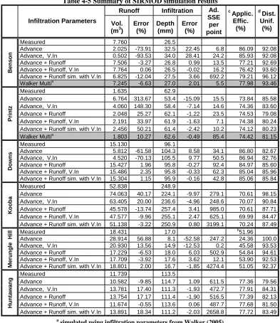
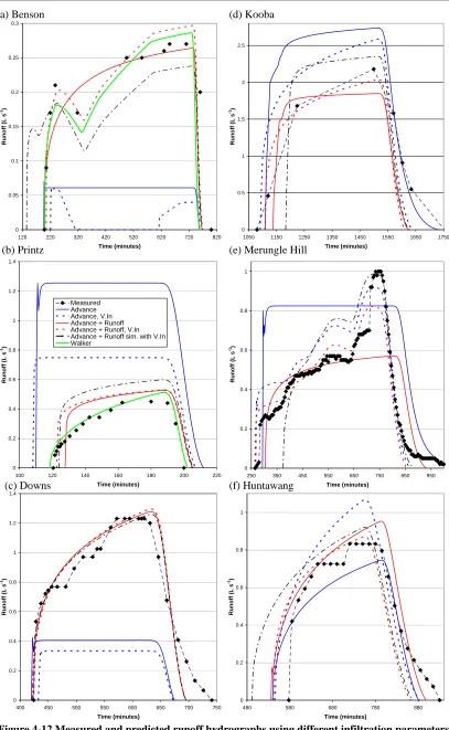
estimated infiltration parameters using the full hydrodynamic model SIRMOD showed that the inclusion of runoff data in the inverse procedure did not compromise the ability to predict the measured advance trajectory but significantly improved the fit to the measured runoff volumes (average decrease in absolute error of simulated runoff volumes of 84%). Whereas the use of runoff data enabled SIRMOD to estimate runoff volumes, accounting for variable inflow improved the fit of the predicted runoff rates to the shape of the measured outflow hydrograph.

Field data collected from several sites across the Darling Downs, Queensland has shown that the infiltration rates vary significantly (e.g. by up to 65% at 500 minutes), both spatially between furrows and temporally over the season. For the sites studied, the spatial variance in infiltration was surpassed by the seasonal variance (e.g. average CV of infiltration of 33.1% compared to 12.5%) but no consistent trends were identified. It was found that the lognormal distribution provided the best fit for the variance in the infiltration curves which was in turn strongly related to the statistical distribution of the infiltration term of the volume balance. From this research, a procedure was developed to predict the infiltration parameters using a single advance point and any number of “known” infiltration curves from the same field.

The IrriProb model was developed to extend the process of simulation from a single furrow scale to the whole field scale. IrriProb performs the full hydrodynamic simulation for multiple independent furrows which are combined to form a spatial representation of the water application. Each furrow can have a unique infiltration rate, inflow rate (Q), time to cut off (TCO) and soil moisture deficit. Validation of IrriProb using multiple sets of field data demonstrated that the single furrow simulations failed to predict the true whole field irrigation performance (e.g. furrow distribution uniformity (DU) between 72.2% and 86.2% compared to the whole field DU of 64.8%).

iv

v

CERTIFICATION OF DISSERTATION

I certify that the ideas, designs, experimental work, software code, results, analyses and conclusions presented in this dissertation are entirely my own effort, except where otherwise indicated and acknowledged.

I further certify that the work is original and has not been previously submitted for assessment in any other course or institution, except where specifically stated.

____________________________ ___________

Malcolm Horace Gillies, Candidate Date

Endorsement:

____________________________ ___________

Prof. Rod Smith, Principal supervisor Date

____________________________ ___________

vi

ACKNOWLEDGEMENTS

The completion of this research is a testimonial to the assistance I have received from a great many people. I would like to take the time here to express my gratitude to some of those who have helped and inspired me during the past three and a half years.

I would like to express my thanks to my supervisors Prof. Rod Smith and Prof. Steven Raine for their guidance during the last few years. I sincerely thank them for their enthusiasm, technical assistance and patience during my PhD studies. Finally I would like to thank Steve and Rod for the proof reading of this dissertation, I know that my English expression can be a little crude at the best of times.

To the staff at the NCEA for their support during my research and help in the collection of irrigation data. In particular to Dr J. McHugh and Dr J. Eberhard for assistance in collection of data for the Lagoona field trial. I would also like to thank John Hornbuckle (CSIRO) for use of his field data. A major part of this research would have not been possible without the simulation model and guidance provided by David McClymont.

I acknowledge the scholarship funding provided by the University of Southern Queensland and the Australian Federal Government. Also to the CRC for Irrigation Futures for providing additional funding for operational costs. I am grateful to the members of the CRC IF for their support and constructive criticism during my study.

To my brother and sisters and especially Mum and Dad who have encouraged me throughout my life. I am forever indebted to you for all your support and inspiration that has led me to this point.

vii

LIST OF PUBLICATIONS FROM THIS

RESEARCH

Gillies, M.H. and Smith, R.J. (2005), Infiltration parameters from surface irrigation advance and run-off data, Irrigation Science, Vol. 24, No.1, pp 25-35.

Gillies, M.H. and Smith, R.J. and Raine, S.R. (2006) Is it possible to extract

infiltration rates for variable inflow furrow irrigation? National Conference, Irrigation Association of Australia. 9-11 May, Brisbane. pp 63-64.

Gillies, M.H. and Smith, R.J. and Raine, S.R. (2007), Accounting for temporal inflow variation in the inverse solution for infiltration in surface irrigation, Irrigation

viii

TABLE OF CONTENTS

ABSTRACT ...II

CERTIFICATION OF DISSERTATION ... V

ACKNOWLEDGEMENTS ...VI

LIST OF PUBLICATIONS FROM THIS RESEARCH... VII

TABLE OF CONTENTS ... VIII

TABLE OF FIGURES... XV

LIST OF TABLES ...XIX

LIST OF ABBREVIATIONS ... XXII

LIST OF SYMBOLS ...XXIII

CHAPTER 1 INTRODUCTION ... 1

1.1 BACKGROUND... 1

1.1.1 Irrigation... 1

1.1.2 Irrigation Performance... 2

1.1.3 Surface Irrigation... 3

1.1.4 Irrigation in Australia ... 6

1.1.5 The Surface Irrigation Debate ... 8

1.1.6 The Issue of Infiltration Variability ... 10

1.2 HYPOTHESIS... 11

1.3 OBJECTIVES... 11

1.4 STRUCTURE OF THIS DISSERTATION... 11

CHAPTER 2 REVIEW OF INFILTRATION AND INFILTRATION VARIABILITY ... 13

2.1 INTRODUCTION... 13

2.2 INFILTRATION... 13

2.2.1 Infiltration Equations... 14

2.3 FACTORS INFLUENCING INFILTRATION... 18

2.3.1 Soil Texture ... 19

2.3.2 Soil Erosion ... 21

2.3.3 Soil Structure and Compaction... 22

2.3.4 Soil Moisture Content and Cracking ... 25

ix

2.3.6 Soil Organisms ... 31

2.3.7 Other Irrigation Water Effects ... 33

2.4 MEASURING SOIL INFILTRATION... 34

2.4.1 Soil Moisture and Laboratory Measurements... 34

2.4.2 Field Infiltrometers... 35

2.4.3 Inverse approach... 39

2.5 INFILTRATION VARIABILITY... 40

2.5.1 Spatial Variability... 41

2.5.2 Seasonal Variability... 43

2.6 EFFECT OF INFILTRATION VARIABILITY ON IRRIGATION PERFORMANCE... 46

2.6.1 Consequence of Assuming Spatially Average Infiltration... 46

2.6.2 Using a Single Furrow to Estimate the Irrigation Performance... 47

2.6.3 Variability and Performance... 47

2.6.4 Impact of Infiltration Variability on Crop Yields and Productivity... 49

2.7 ESTIMATING INFILTRATION RATES WHILE ACCOUNTING FOR INFILTRATION VARIABILITY... 51

2.7.1 Relating Infiltration to Other Parameters... 51

2.7.2 Estimating Infiltration Variability through Statistical Analysis ... 52

2.7.3 Real-Time Estimation of Infiltration Parameters... 56

2.7.4 Cost of Sampling ... 56

2.7.5 Accuracy versus Sample Number... 57

2.8 IRRIGATION STRATEGIES TO REDUCE INFILTRATION VARIABILITY AND/OR IMPROVE PERFORMANCE... 58

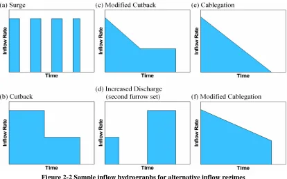
2.8.1 Surge Irrigation... 58

2.8.2 Cutback Irrigation... 61

2.8.3 Increased Discharge... 62

2.8.4 Alternate and Wide Spaced Furrow... 62

2.8.5 Cablegation... 64

2.8.6 Deficit Irrigation... 64

2.8.7 Real-Time Control... 65

2.8.8 Application of Polyacrylamide ... 67

2.9 CONCLUSION... 67

CHAPTER 3 HYDRAULIC SIMULATION OF FURROW IRRIGATION... 69

3.1 PURPOSE OF THE SIMULATION MODEL... 69

3.1.1 Identification of Field Characteristics ... 69

3.1.2 Evaluation of the Current Irrigation Performance ... 69

3.1.3 Optimisation of Field Design and Management ... 70

3.2 HYDRAULIC MODEL THEORY... 70

3.2.1 Full Hydrodynamic Model ... 72

x

3.2.3 Kinematic Wave Model... 73

3.2.4 Volume Balance Model ... 73

3.2.5 Simulating Longitudinal (Within Furrow) Variation... 74

3.3 ESTIMATING INFILTRATION THROUGH INVERSE SIMULATION OF SURFACE IRRIGATION... 76

3.3.1 Full Hydrodynamic Model ... 76

3.3.2 Zero Inertia Model... 77

3.3.3 Volume Balance Model ... 77

3.3.4 Discussion of the Inverse Procedures ... 79

3.4 APPARENT INFILTRATION VARIABILITY IN THE INVERSE SOLUTION AND SIMULATION PROCESSES... 80

3.4.1 Inflow Rate ... 80

3.4.2 Wetted Perimeter ... 82

3.4.3 Surface Storage... 85

3.5 SIMULATION MODELS TO EVALUATE AND OPTIMISE PERFORMANCE... 86

3.5.1 SIRMOD ... 86

3.5.2 SRFR ... 87

3.5.3 FIDO... 87

3.5.4 Other Models ... 88

3.6 CONCLUSIONS... 89

CHAPTER 4 DEVELOPMENT OF IPARM ... 90

4.1 INTRODUCTION... 90

4.2 VOLUME BALANCE MODEL FOR INVERSE SOLUTION OF INFILTRATION... 91

4.2.1 Volume Balance Model ... 91

4.2.2 Advance Phase ... 91

4.2.3 Runoff Phase ... 97

4.2.4 Variable Inflow... 99

4.3 IPARMMODEL DEVELOPMENT... 101

4.3.1 Advance Phase ... 101

4.3.2 Runoff Phase ... 103

4.3.3 Depletion and Recession Phases... 105

4.3.4 Variable Inflow... 107

4.3.5 Objective function ... 111

4.3.6 Solution Scheme... 112

4.3.7 The IPARM Computer Software ... 115

4.4 EVALUATION OF IPARM ... 117

4.4.1 Input Data ... 117

4.4.2 Estimation of Infiltration Parameters... 121

4.4.3 Validation of the Surface Storage Smoothing Approach... 127

xi

4.5.1 Prediction of Advance Trajectory... 130

4.5.2 Prediction of the Runoff Hydrograph ... 133

4.5.3 Prediction of Irrigation Performance and Distribution of Infiltrated Depths... 135

4.6 INFLOW AS A SOURCE OF VARIABILITY IN SPATIAL ESTIMATES OF INFILTRATION... 137

4.7 SENSITIVITY OF IPARM TO SECTION OF INPUT DATA POINTS... 140

4.7.1 Introduction ... 140

4.7.2 Selection of Advance Measurements... 141

4.7.3 Selection of Runoff Measurements ... 142

4.7.4 Weighting of Runoff Compared to Advance Data ... 144

4.8 DISCUSSION... 145

4.8.1 Data Collection Recommendations ... 145

4.8.2 IPARM User Intervention ... 147

4.8.3 Parameter Starting Estimates... 148

4.8.4 Conclusion... 148

CHAPTER 5 FIELD VARIABILITY OF INFILTRATION... 150

5.1 INTRODUCTION... 150

5.2 PREVIOUS ATTEMPTS TO ASSESS INFILTRATION VARIABILITY... 151

5.3 DESCRIBING INFILTRATION VARIABILITY WITH STATISTICAL TECHNIQUES... 152

5.3.1 Review of Statistical Distribution Models... 152

5.3.2 Sampling Distribution, a Tool to Determine Required Number of Measurements ... 156

5.4 MULTIPLE FURROW FIELD DATA... 157

5.4.1 Collection of Field Data using Irrimate™ Equipment... 157

5.4.2 Downs... 159

5.4.3 Chisholm ... 160

5.4.4 Turner ... 160

5.4.5 Additional Field Data for Seasonal Trends... 161

5.4.6 Estimating Surface Storage using Manning’s n... 161

5.5 ESTIMATION OF THE INFILTRATION CURVES... 162

5.5.1 Downs... 162

5.5.2 Chisholm ... 163

5.5.3 Turner ... 164

5.6 VARIABILITY OF INFILTRATION... 166

5.6.1 Variability between Infiltration Curves ... 166

5.6.2 Seasonal (Between Irrigation Events) Infiltration Variability ... 167

5.6.3 Significance of Temporal and Spatial Variability ... 170

5.6.4 Seasonal Compared to Spatial Variability ... 171

5.7 MINIMUM NUMBER OF INFILTRATION CURVES REQUIRED TO ESTIMATE WHOLE FIELD VARIABILITY... 173

xii

5.7.2 Sampling Distributions ... 174

5.7.3 Number of Field Samples Required to Reach a Given Accuracy... 176

5.8 DESCRIBING INFILTRATION VARIABILITY USING STATISTICAL DISTRIBUTION FUNCTIONS.. 181

5.8.1 Statistical Test Methodology ... 181

5.8.2 Downs... 182

5.8.3 Chisholm ... 185

5.8.4 Turner ... 186

5.8.5 Discussion ... 187

5.9 ESTIMATING INFILTRATION USING PROBABILITY... 188

5.9.1 Development of an Infiltration Prediction Procedure... 189

5.9.2 Validation of the Infiltration Prediction Procedure ... 195

5.9.3 The Predictive Procedure Compared to Scaling ... 199

5.10 CONCLUSIONS... 200

CHAPTER 6 WHOLE FIELD SIMULATION MODEL ... 202

6.1 INTRODUCTION... 202

6.2 COMPONENTS OF THE SIMULATION MODEL... 203

6.2.1 Introduction to IrriProb... 203

6.2.2 FIDO Simulation Engine ... 204

6.2.3 Calculation of Performance Parameters ... 206

6.2.4 Calculation and Visualisation of the Whole Field Performance... 210

6.3 SURFACE IRRIGATION OPTIMISATION FRAMEWORK... 212

6.3.1 Development of the Optimisation Tool ... 212

6.3.2 Validation of the IrriProb Simulation Model... 215

6.4 SIMPLE FURROW AVERAGES CANNOT REPRESENT THE FIELD PERFORMANCE... 216

6.5 IRRIGATION PERFORMANCE IN HETEROGENEOUS CONDITIONS UNDER MEASURED FIELD MANAGEMENT... 218

6.6 CONCLUSION... 220

CHAPTER 7 OPTIMISING IRRIGATION PERFORMANCE CONSIDERING INFILTRATION VARIABILITY... 222

7.1 INTRODUCTION... 222

7.2 THE FURROW IRRIGATION OPTIMISATION PROCESS... 223

7.2.1 Factors to Consider in Addition to the Standard Performance Terms ... 223

7.2.2 Existing Techniques to Optimise Irrigation Management ... 225

7.2.3 Optimising Irrigation Performance at the Field Scale ... 226

7.3 THE OPTIMISATION OBJECTIVE FUNCTION... 227

7.3.1 Arithmetic Objective Function ... 227

7.3.2 Boolean Objective Function ... 229

7.3.3 Optimisation Methodology... 230

xiii

7.4.1 Interactions between Inflow and Performance ... 231

7.4.2 The Trade-off between the Performance Terms in the Objective Function... 234

7.4.3 Movement of the Optimised Point in the Inflow Rate/Inflow Time Domain ... 237

7.5 CAN THE OPTIMAL FIELD MANAGEMENT BE IDENTIFIED FROM A SINGLE FURROW? ... 240

7.5.1 Introduction ... 240

7.5.2 Furrow Based Performance Terms Compared to Field Values ... 240

7.5.3 Example: Optimising the Downs Field using Opt 1 ... 242

7.5.4 Summary of Results ... 244

7.5.5 Optimising Using the Average Infiltration Curve ... 246

7.6 IMPROVING THE PERFORMANCE OF FURROW IRRIGATION USING RECIPE MANAGEMENT STRATEGIES... 247

7.7 OPTIMISING IRRIGATION MANAGEMENT IN HETEROGENEOUS CONDITIONS USING THE WHOLE FIELD APPROACH... 250

7.8 RELATIONSHIPS BETWEEN INDIVIDUAL FURROW OPTIMA AND THE WHOLE FIELD OPTIMUM... ... 252

7.9 CONCLUSION... 256

CHAPTER 8 PRACTICAL DEMONSTRATION: THE LAGOONA FIELD TRIAL . ... 259

8.1 INTRODUCTION... 259

8.2 FIELD DATA... 259

8.3 CALIBRATION OF THE INFILTRATION CURVE... 262

8.3.1 Estimation of Infiltration Curves using IPARM... 262

8.3.2 Minimum Distance for Field Measurement... 263

8.3.3 Predicting Infiltration Parameters using the Final Advance Time... 265

8.4 OPTIMISING PERFORMANCE... 266

8.4.1 Current Performance ... 266

8.4.2 Optimising the Time to Cut-off ... 268

8.4.3 Optimising Inflow ... 269

8.5 SENSITIVITY OF OPTIMISATION PROCESS TO UNCERTAINTIES IN FIELD MEASUREMENTS.... 270

8.6 CONCLUSIONS... 271

CHAPTER 9 CONCLUSIONS AND RECOMMENDATIONS... 272

9.1 CONCLUSIONS FROM THIS RESEARCH... 272

9.1.1 Estimation of Infiltration Parameters from Field Measurements... 272

9.1.2 Statistical Nature of Infiltration Variability... 274

9.1.3 Whole Field Simulation and Optimisation Model ... 275

9.2 KEY RESEARCH OUTCOMES... 278

9.3 RECOMMENDATIONS FOR FURTHER RESEARCH... 278

9.3.1 Inverse Techniques to Estimate Infiltration... 279

xiv

9.3.3 Statistical Description of Infiltration Variability ... 281

9.3.4 Simulation Models for Heterogeneous Conditions... 281

LIST OF REFERENCES ... 283

APPENDIX A FIELD DATA FOR IPARM VALIDATION... 295

APPENDIX B C++ CODE FOR KOSTIAKOVCALIBRATIONOBJECT... 307

APPENDIX C EXTRA RESULTS FOR IPARM VALIDATION ... 332

APPENDIX D FIELD DATA FOR INFILTRATION VARIABILITY AND WHOLE FIELD SIMULATION ... 335

APPENDIX E RESULTS FROM SAMPLE SIZE ANALYSIS ... 346

APPENDIX F RESULTS FROM INFILTRATION PREDICTION... 349

APPENDIX G VALIDATION OF THE FIDO SIMULATION ENGINE USED BY IRRIPROB ... 352

APPENDIX H IRRIPROB: IRRIGATION PERFORMANCE UNDER MEASURED CONDITIONS... 358

xv

TABLE OF FIGURES

Figure 1-1 Large scale level basin irrigation of rice/wheat field in Griffith region, southern

NSW ...5

Figure 1-2 Furrow irrigation of cotton near Moree, northern NSW showing siphon application ...5

Figure 2-1 Cross section view of the (a) single ring and (b) double ring infiltrometer (Reynolds et al. 2002) ...36

Figure 2-2 Sample inflow hydrographs for alternative inflow regimes ...58

Figure 3-1 Control volume for Saint-Venant equations...71

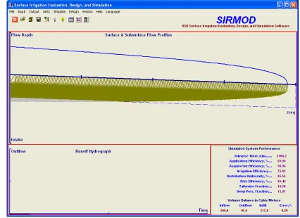
Figure 3-2 Screenshot of SIRMOD III: simulation of the Kooba field with variable inflow (infiltration estimated using advance and runoff with variable inflow) ...86

Figure 4-1 Volume balance model during the advance phase ...91

Figure 4-2 Explanation of the Surface Storage Smoothing calculation ...110

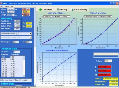
Figure 4-3 Screen shot of main user interface for IPARM version 1.1.2...116

Figure 4-4 Screen shot of main user interface for IPARM version 2 ...116

Figure 4-5 Measured inflow hydrographs for IPARM validation...119

Figure 4-6 Calibrated infiltration curves for IPARM validation...124

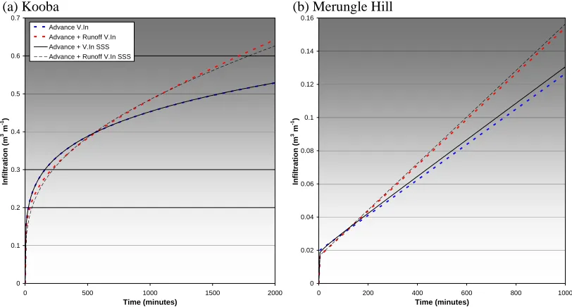
Figure 4-7 Cumulative infiltrated volumes comparing infiltration from the volume balance (actual/measured) with predicted infiltration from parameters estimated from the advance and storage phases ...126

Figure 4-8 Comparing infiltration curves estimated using the variable inflow hydrograph between original surface storage and surface storage smoothing (SSS) technique ...128

Figure 4-9 Comparing the surface storage smoothing (SSS) calculation with the standard variable and constant inflow approach (Merungle Hill data) ...129

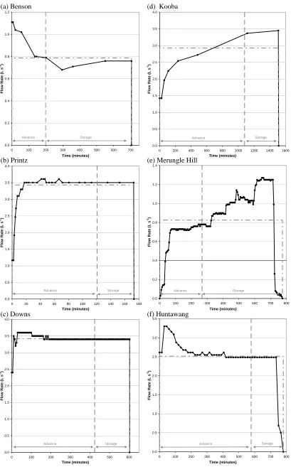
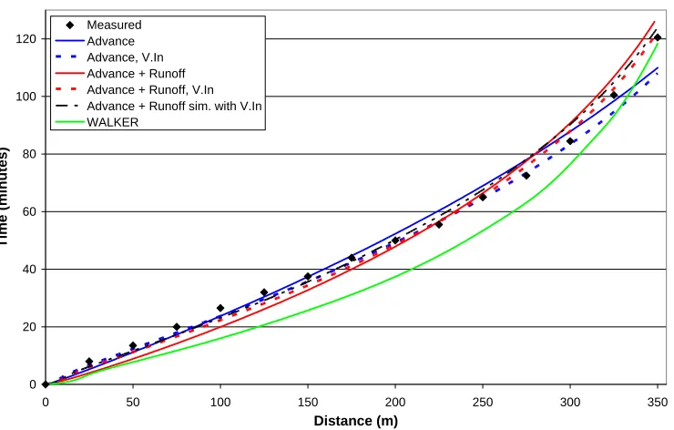
Figure 4-10 Measured and SIRMOD simulated advance (Benson data) ...131

Figure 4-11 Measured and SIRMOD simulated advance (Printz data) ...131

Figure 4-12 Measured and predicted runoff hydrographs using different infiltration parameters ...134

Figure 4-13 Effect of infiltration parameter estimation on the predicted water depth profile (Merungle Hill data)...137

Figure 4-14 Measured inflow hydrographs for Kooba site ...138

Figure 4-15 Infiltration curves for the Kooba site estimated using advance data with constant inflow ...139

xvi

Figure 4-17 Infiltration curves estimated using different advance measurements (Merkley

data)...143

Figure 4-18 Infiltration curves estimated using different runoff measurements (Merkley data)...143

Figure 4-19 Sensitivity of IPARM to the weighting (w) between runoff and advance errors (Merkley data) ...145

Figure 5-1 Irrimate™ siphon flow meter ...158

Figure 5-2 Irrimate™ advance sensor...158

Figure 5-3 Irrimate™ flume flow meter ...158

Figure 5-4 Infiltration curves estimated from advance and runoff with constant inflow (Downs field)...163

Figure 5-5 Infiltration curves estimated from advance with constant inflow (Chisholm field) ...165

Figure 5-6 Infiltration curves estimated from advance with constant inflow (Turner field) ...165

Figure 5-7 CV of infiltration with opportunity time (Downs, Chisholm and Turner fields) ...167

Figure 5-8 Sampling distribution of mean of Z with increasing sample size (Downs field) ...174

Figure 5-9 Sampling distribution of standard deviation of Z with increasing sample size (Downs field)...175

Figure 5-10 Sampling distribution of mean of Z using 900 random samples for each sample size (Downs field) ...176

Figure 5-11 Maximum relative error in the estimated population mean (Eµ) according to sample size ...178

Figure 5-12 Maximum relative error in the estimated standard deviation (Eσ) according to sample size ...179

Figure 5-13 Frequency histograms of cumulative infiltration at 615.1 minutes opportunity time (Downs field) ...183

Figure 5-14 Log-normal probability plot of cumulative infiltration at 615.1 minutes with (a) all furrows and (b) outlier removed (Downs field) ...183

Figure 5-15 Frequency histograms of cumulative infiltration at 230 and 800 minutes opportunity time (Chisholm field)...185

Figure 5-16 Frequency histograms of cumulative infiltration at 500 and 1000 minutes opportunity time (Turner field) ...187

xvii

Figure 5-18 Correlation of CV between logarithm infiltration and logarithm of volume

balance...194

Figure 5-19 Comparing predicted and IPARM estimated infiltration curves (Downs field,

using Irr1Fur1) ...196

Figure 5-20 Comparison between infiltration depths from the predictive procedure and those

estimated using IPARM (actual) ...197

Figure 6-1 IrriProb screen shot: Simulation of Turner field ...204

Figure 6-2 Three dimensional IrriProb plots of (a) infiltration, (b) root zone and (c) deep

drainage (Downs trial site under measured conditions) ...211

Figure 6-3 Batch simulation parameter input box...212

Figure 6-4 Screenshot from IrriProb: Performance indicators for Downs field (Q = 1 to 11

L s-1 and TCO = 200 to 1200 minutes)...213

Figure 6-5 Screenshot from IrriProb continued: Performance indicators for Downs field (Q

= 1 to 11 L s-1 and TCO = 200 to 1200 minutes) ...214

Figure 6-6 IrriProb screen shot: Using the optimising tool to determine inflows that

achieve RE>90%, DURZ>90% and AE>65% (Downs field)...214

Figure 7-1 Optimising using an Arithmetic objective function: ¼(RE) ¼AE) + ¼DU +

¼(1-DD%) (Downs field)...228

Figure 7-2 Cut-off time plotted against application efficiency and requirement efficiency

(Downs field)...232

Figure 7-3 Inflow rate plotted against application efficiency and requirement efficiency

(Downs field)...233

Figure 7-4 Behaviour of the objective function of a) Opt 1 and b) Opt 2 (Downs field) .235

Figure 7-5 Behaviour of AE in relation to RE and DURZ (Downs field) ...236

Figure 7-6 Behaviour of DDD in relation to RE and AE (Downs field)...236

Figure 7-7 Movement of the optimal inflow point to maximise application efficiency while

varying the RE and DURZ criteria (Downs field)...238

Figure 7-8 Movement of the optimal inflow point to minimise deep drainage while varying

the RE and AE criteria (Downs field) ...239

Figure 7-9 Comparing the inflow rates and times that meet each performance criteria for

Opt 1 (a – c) and Opt 2 (c - d) and DU = 80% between the individual furrows and the whole field ...241

Figure 7-10 Relationship between the optimised Q and TCO amongst individual furrows

and the field optimum for the Downs field using Opt 1...252

Figure 7-11 Relationship between the optimised Q and TCO amongst individual furrows

and the field optimum for the Chisholm field using Opt 1 and Opt 2 ...253

Figure 7-12 Log-Log relationships between optimised Q and TCO for each single furrow

xviii

Figure 8-1 Advance meter at 0 m (head-ditch) in Lagoona trial...260

Figure 8-2 Lagoona field trial layout ...261

Figure 8-3 Time taken to reach final advance point (761 m) for the Lagoona field ...262

Figure 8-4 Infiltration curves for Lagoona estimated using IPARM ...263

Figure 8-5 Correlogram of final advance times (761 m) for Lagoona...264

Figure 8-6 Predicted infiltration curves for Lagoona...266

Figure E.1 Chisholm: Sampling distributions of the mean ...347

Figure E.2 Chisholm: Sampling distributions of the standard deviation...347

Figure E.3 Turner: Sampling distributions of the mean...348

Figure E.4 Turner: Sampling distributions of the standard deviation ...348

Figure G.1 Simulated advance trajectories (Downs, Irr2 Fur3) ...354

Figure G.2 Simulated runoff hydrographs (Downs, Irr2 Fur3) ...354

xix

LIST OF TABLES

Table 1-1 Irrigation area, volume and type by state (Created from data included in ABS

2006b)...7

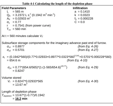
Table 4-1 Calculating the length of the depletion phase...106

Table 4-2 Default starting estimates and initial step sizes for IPARM...113

Table 4-3 Infiltration parameters and volume balance errors for IPARM validation...122

Table 4-4 Infiltration parameters from IPARM using the surface storage smoothing (SSS) approach ...128

Table 4-5 Summary of SIRMOD simulation results ...132

Table 4-6 Advance data for sensitivity analysis (Merkley data) ...141

Table 4-7 Runoff hydrograph for sensitivity analysis (Merkley data)...141

Table 4-8 Sensitivity of infiltration parameters to the runoff weighting factor (Merkley data)...144

Table 4-9 Infiltration parameters for Downs using different starting parameter estimates ...148

Table 5-1 Infiltration parameters for Downs (whole field) ...162

Table 5-2 Infiltration parameters (Chisholm field)...164

Table 5-3 Infiltration parameters (Turner field) ...164

Table 5-4 Seasonal correlation between infiltration parameters and infiltrated depths...168

Table 5-5 Seasonal correlation of infiltrated depths with irrigation number...170

Table 5-6 Significance of temporal variability using ANOVA ...171

Table 5-7 Comparison between spatial and seasonal variability (coefficient of variation) ...171

Table 5-8 Statistical summary of infiltration curves and test for normality considering both (a) all data and (b) outlier removed (Downs field)...184

Table 5-9 Statistical summary of infiltration curves and test for normality (Chisholm field) ...186

Table 5-10 Statistical summary of infiltration curves and test for normality (Turner field) ...187

Table 5-11 Comparison between actual (IPARM estimated) and predicted infiltration curves ...198

Table 6-1 Differences in the performance indicators between simple furrow averages and the true field performance (Downs field) ...217

Table 6-2 Field irrigation performance under the measured irrigation management ...219

xx

Table 7-2 Average difference (overestimation) between the single furrow and the field

performance simulated with the individual furrow optimum management ....245

Table 7-3 Average infiltration parameters for Downs, Chisholm and Turner...246

Table 7-4 Optimising inflow rates and TCO using the average infiltration curve ...247

Table 7-5 Irrigation performance with various different recipe management strategies for the (a) Downs, (b) Chisholm and (c)Turner fields ...249

Table 7-6 Optimising irrigation inflow rates and TCO considering the whole field ...250

Table 8-1 Optimising Lagoona by time to cut-off ...268

Table 8-2 Optimising Lagoona by time inflow rate and time to cut-off...269

Table A.1 Field data for Benson ...296

Table A.2 Field data for Printz...297

Table A.3 Field data for Downs (Irrigation 2 Furrow 3)...298

Table A.4 Field data for Kooba...299

Table A.5 Field data for Merungle Hill...300

Table A.6 Field data for Huntawang ...302

Table A.7 Field data for Merkley...303

Table A.8 All advance data for Kooba...304

Table A.9 All inflow data for Kooba ...305

Table A.10 All runoff data for Kooba...306

Table C.1 Infiltration parameters for Kooba from advance with constant and variable inflow ...333

Table C.2 Infiltration parameters for Kooba from advance and runoff data with constant and variable inflow...333

Table C.3 Infiltration parameters for Merkley estimated by selecting different advance measurements ...334

Table C.4 Infiltration parameters for Merkley estimated by selecting different runoff measurements ...334

Table D.1 Field data for Downs (whole field) ...336

Table D.2 Runoff data for Downs (whole field) Irr1 Fur1 – Irr2 Fur3 ...337

Table D.3 Runoff data for Downs (whole field) Irr2 Fur4– Irr4 Fur4 ...338

Table D.4 Runoff data for Downs (whole field) Irr5 Fur1 – Irr5 Fur4 ...339

Table D.5 Field data for Chisholm...340

xxi

Table D.7 Field data and infiltration parameters for Coulton A ...342

Table D.8 Field data and infiltration parameters for Coulton B...343

Table D.9 Field data for and infiltration parameters for Coulton C ...344

Table D.10 Field data and infiltration parameters for Turner Field 18 ...345

Table F.1 Estimated infiltration parameters for Downs ...350

Table F.2 Estimated infiltration parameters for Chisholm ...350

Table F.3 Estimated infiltration parameters for Turner...351

Table G.1 Comparison of SIRMOD and IrriProb Performance Terms...356

Table H.1 Downs: irrigation performance under measured conditions ...359

Table H.2 Chisholm: irrigation performance under measured conditions using a constant deficit equal to 0.06 m...359

Table H.3 Chisholm: irrigation performance under measured conditions using measured (variable) soil water deficits ...360

Table H.4 Turner: irrigation performance under measured conditions ...360

Table I.1 Downs Opt 2: RE>95%, AE>70% and DDD is minimised ...362

Table I.2 Chisholm Opt 1: RE>90%, DURZ>90% and AE is maximised ...363

Table I.3 Chisholm Opt 2: RE>95%, AE>60% and DDD is minimised ...363

Table I.4 Chisholm Opt 3: RE>95%, AE>60% and DDD is minimised with variable irrigation requirement...364

Table I.5 Turner Opt 1: RE>90%,DURZ>90% and AE is maximised...365

Table I.6 Turner Opt 2: RE>95%, AE>70% and DDD is minimised...366

Table I.7 Recipe field performance ...367

Table J.1 Advance data for Lagoona Trial...369

Table J.2 Runoff data for Lagoona Trial...370

Table J.3 Infiltration parameters for Lagoona from IPARM ...371

Table J.4 Infiltration parameters predicted using final advance point ...372

xxii

LIST OF ABBREVIATIONS

ADU absolute distribution uniformity AE application efficiency

AELQ application efficiency of the low quarter

AER application efficiency accounting for tail water recycling

AT average advance time (time of the final advance point for a set of furrows) CV coefficient of variation

CU Christiansen's uniformity coefficient

DD deep drainage/deep percolation below the root zone DDD average depth of deep drainage

DU low quarter distribution uniformity DURZ distribution uniformity of the root zone EC electrical conductivity

EM electromagnetic survey ESP exchangeable sodium percentage

ETc crop evapo-transpiration calculated from the reference evaporation FIDO Furrow Irrigation Design Optimiser

Fur furrow

GPS global positioning system

IPARM infiltration parameters from advance and runoff model Irr irrigation

MIC model infiltration curve

NCEA National Centre for Engineering in Agriculture NSW New South Wales

Opt optimisation (objective function to optimise performance) PAM Polyacrylamide

PRD partial root-zone drying Q inflow rate Qld Queensland

RE requirement efficiency RMSE root mean square error SAR sodium adsorption ratio SCS US Soil Conservation Service SSE standard square error

xxiii

LIST OF SYMBOLS

α significance level

β curvature constant for surface water storage

γ semivariance

ζ empirical exponent of Q for variation of infiltration with inflow

η dynamic viscosity (Pa s)

θ decrease in infiltration over time from Horton equation

λ ratio of current time to end of advance µ population mean

σ population standard deviation

σs sample standard deviation

σy surface storage coefficient for advance

phase

σys surface storage coefficient for storage

phase

σz1 subsurface storage coefficient of the

transient infiltration term

σz2 subsurface storage coefficient of the

steady infiltration term

τ infiltration opportunity time (min)

0

f

τ time constant of the Branched Kostiakov equation

φ empirical parameter for variation of infiltration with wetted perimeter

χ2

chi squared statistic

ωCV coefficient to calculate CVInfiltration from

CVVB

ωZVal coefficient to calculate ZValInfiltration from

ZValVB

a empirical Kostiakov/Modified Kostiakov infiltration parameter

A cross-sectional area of flow (m2)

A0 upstream area of flow (m2)

ACF autocorrelation coefficient

AT average time value of the last measured advance point (min)

c coefficient of the power relationship of furrow width to depth

C crack infiltration term (m3 m-1)

CVInfiltration time averaged CV for the

logarithm of the Modified Kostiakov infiltration

CVVB CV for the logarithm of the infiltration

term of the volume balance

D volume of infiltration per unit area of soil (m)

LQ

D average of D over the quarter of the field with the lowest infiltration (m)

LQ

RZ

D average of DRZ over the quarter of the

field with the lowest infiltration (m)

DDD volume of deep drainage per unit area of

soil (m)

Dmin minimum value of D across the field (m)

Dreq required volume of infiltration per unit

area or soil moisture deficit (m)

DRZ volume infiltrated and stored in the root

zone per unit area of soil (m)

E[] the expected value

ER efficiency of the tail-water recycling

system

f0 semi-empirical steady state infiltration

parameter of the Modified Kostiakov (m3 m-1 min-1)

F rapid surface storage term from the Horton equation

FS scaling factor of infiltration function for

the MIC approach

g acceleration due to gravity (9.81 m s-2)

G group iteration factor (default = 0.01)

h lag distance (between samples)

H pressure head (m)

I infiltration rate (m3 m-1 min-1)

ICF irrigation condition factor

xxiv

Jatemp record of Ja for the last round of

individual parameter searches

JC equivalent to Ja butfor C JCtemp equivalent to Jatemp butfor JC

Jf0 equivalent to Ja butfor f0

Jf0temp equivalent to Jatemp but for Jf0

Jk equivalent to Ja butfor k

Jktemp equivalent to Jatemp butfor Jk

k empirical Kostiakov/Modified Kostiakov infiltration parameter (m3 m-1 min-a)

K hydraulic conductivity (m3 m-2 min-1)

Ks saturated hydraulic conductivity (m3 m-2

min-1)

Kwet hydraulic conductivity at field capacity

(m3 m-2 min-1)

L field length (m)

m exponent of the power relationship of furrow width to depth.

n Manning roughness coefficient

N number of data points

Na number of advance points

Nr number of runoff points

OBJ objective function for optimisation of irrigation management

p parameter of the power advance function

P wetted perimeter (m)

P0 upstream wetted perimeter (m)

qr steady runoff rate (m3 min-1)

Q discharge (m3 s-1)

Q0 inflow rate at upstream end of furrow

(m3 min-1)

Qr outflow discharge (m3 s-1)

Qx flow rate at point x in a furrow (m3 s-1)

r exponent of power advance function

R Pearson correlation coefficient

s distance measured from the upstream end of the field (m)

sZ2 variance of Z

S sorptivity as present in the Phillip equation

S0 field slope

Sf friction slope

t time (min or sec)

tStat t statistic from the t-distribution

tx time taken to reach point x (min)

tw time taken for a change in upstream area

to have effect over the wetted furrow length (min)

Tadvance length of the advance phase at the

current time (min)

Tdepletion length of the depletion phase (min)

v flow velocity (m s-1)

vx flow velocity at point x (m s-1)

Vf volume surface storage at end of storage

phase (m3)

VI volume of infiltration (m3)

VR volume of runoff (m3) i

R

V measured runoff volume at data point, i

(m3)

VS volume of surface storage (m3)

Vw velocity of a wave or small disturbance

(m s-1)

VZx volume of infiltration at the time tx (m3)

VolDD volume of infiltration that drains below

the rootzone as deep percolation (m3)

VolInfiltration volume of infiltration (m3)

VolRZ volume of infiltration stored in the root

zone (m3)

Volreq volume of infiltration required to refill

the rootzone (m3)

VolRunoff volume of runoff (m3)

VolInflow volume of inflow (m3)

w weighting factor for advance and runoff errors in IPARM (%)

W top width of flow within the furrow (m)

WB bottom width of the furrow (m)

WM furrow width at half the total height (m)

Ws furrow spacing (m)

WT furrow width at the total height (m)

x advance distance (m)

xi measured advance distance at data point,

xxv

xt predicted advance distance if the

advance continued beyond the end of the field (m)

X a continuous variable

Xi a continuous variable measured at point i

y depth of flow (m)

y0 upstream depth of flow (m)

YT total height of furrow (m)

y centroid of the area of flow (m)

yw depth of the wetting front (m)

Z infiltrated depth per unit length of furrow (m3 m-1)

ZS scaled infiltration depth per unit length

of furrow (m3 m-1)

Zx infiltrated depth at distance x (m3 m-1)

ZVal standard normal variate

ZValInfiltration time averaged ZVal for the

logarithm of the Modified Kostiakov infiltration

ZValVB ZVal for the logarithm of the infiltration

1

CHAPTER 1

Introduction

This thesis deals with the issue of infiltration variability and its influence over the performance and management of surface irrigation. As such, this introductory chapter establishes the purpose and importance of irrigation whilst covering the characteristics of different application systems. The concise discussion herein provides the necessary background to define the objectives of this research.

1.1 Background

1.1.1 Irrigation

Irrigation is defined by the Oxford English dictionary (Simpson and Weiner 1989) as “The action of supplying land with water by means of channels and streams; the distribution of water over the surface of the ground in order to promote the growth and productiveness of plants”. Water is required by almost every aspect of life on Earth. It makes up a large proportion of all plant and animal tissue, serves as the essential for the fundamental processes of photosynthesis and respiration.

Through history, humans have learnt to use irrigation to enhance the production and reliability of crops and facilitate the growing of many plants outside their natural environment. Full irrigation describes the situation where little or no effective rainfall occurs during the growing season and all moisture must be supplied artificially. Supplementary irrigation differs in that water is applied in order to complement the natural precipitation and is often preferred over the full irrigation strategy.

2

plains between the Tigris and Euphrates Rivers in modern day Iraq. The crops germinated but the lack of follow up rain caused them to wither and die. The farmers fixed this problem by digging a network of channels and ditches to supply water to the fields (Postel 1999). These early irrigation systems resembled what we now call flood and furrow irrigation. The Egyptians and Indians pioneered a system of “inundation canals” that are dug parallel to the river and rely on regular seasonal flooding (Cantor 1970). In Egypt, these canals were used to supply water to the field in a basin type irrigation where the water was ponded on the soil surface and later drained. Basin irrigation can still be seen relatively unchanged in the region to this day. Irrigation must have been an integral part of the Egyptian civilisation as a historic relief dated from 3,100 BC shows the Scorpion King using a hoe to cut a ditch in a network grid (Postel 1999). Evidence for similar primitive irrigation systems has also been found in other regions such as China and Mexico. The advent of irrigation was a turning point for society as it assisted farmers to produce excess food and therefore freed up labour. These non-farm workers could then pursue other occupations in areas diverse as from metalworking to mathematics. Considering this, irrigated agriculture led to the creation of the urban society that is so prevalent in the modern age.

Crops have been grown with the aid of irrigation for thousands of years but technological advances over the past few centuries have provided farmers with new techniques to apply water to the field. The wide range of irrigation techniques can be grouped into three main categories, namely surface, sprinkler and drip irrigation. This dissertation deals with surface irrigation systems.

1.1.2 Irrigation Performance

3

application efficiency, volume added to the root zone divided by the total applied. Uniformity refers to the spatial distribution of infiltrated depths and is typically expressed in terms of the distribution uniformity, average low quarter divided by the average infiltrated depth or the coefficient of uniformity, average deviation from the mean of applied depths.

1.1.3 Surface Irrigation

Surface irrigation is defined as the group of application techniques where water is applied and distributed over the soil surface by gravity. It is the oldest technique and is also the simplest to implement. Surface irrigation is often referred to as flood irrigation, implying that the water distribution is uncontrolled and therefore, inherently inefficient. In reality, the various irrigation practices grouped under this name often involve some degree of management. In some cases (e.g. surge irrigation), the implementation of surface irrigation actually demands a high level of control and expertise. Surface irrigation is further divided into the three types; level basin, border strip and furrow irrigation, which is the primary focus of this dissertation.

1.1.3.1Level Basin

4

1.1.3.2Furrow

Furrow irrigation is the most common form of irrigation throughout the world (Burt 1995). The furrow itself is a small trench, typically between 200 to 800 millimetres wide, 100 to 300 millimetres deep and orientated in the direction of predominant slope. They are traditionally closely spaced with the plants located on the crest of the ridge between adjacent furrows. Alternatively, the field may be formed into beds, which are flat elevated regions between the furrows rather than a single narrow ridge. The actual distance between furrows is governed by a combination of the plant spacing, machinery track-width, irrigation management and the soils capacity for horizontal redistribution of water. Shorter furrows are commonly associated with higher uniformity of application and increased potential for runoff losses. However, farmers in Australia tend towards longer furrows (e.g. 950m in Figure 1-2) to reduce the labour requirements and to minimise the area of land occupied by irrigation infrastructure.

5

by extending the furrow upstream into the head ditch. Water automatically flows into each furrow when the depth in the head-ditch is higher than the bottom of the furrow cross-section.

Figure 1-1 Large scale level basin irrigation of rice/wheat field in Griffith region, southern NSW

Figure 1-2 Furrow irrigation of cotton near Moree, northern NSW showing siphon application

6

1.1.3.3Border Strip

Border strip or bay irrigation could be considered as a hybrid of level basin and furrow irrigation. The borders of the irrigated strip are longer and the strips are narrower than for basin irrigation and are orientated to align lengthwise with the slope of the field. The water is applied to the top end of the bay, which is usually constructed to facilitate free-flowing conditions at the downstream end.

1.1.4 Irrigation in Australia

Australia is often given the title of the driest continent on earth, and in reality it is only surpassed by Antarctica. Situated approximately 30° from the equator positions Australia on the latitudes that contain a large portion of the desert regions of the world, including the Sahara and Arabian deserts. These zones are characterised by lower rainfall due to the persistent high pressures caused by dry colder air sinking from high altitudes as part of the Hadley Cell system (Hidore and Oliver 1993). The majority of Australia receives low rainfall and experiences high rainfall variability from season to season. It is therefore necessary for many farmers to look to irrigation in order to minimise the risk associated with agricultural production.

Irrigation emerged in many locations in Australia during the 19th century but was generally limited to individuals or small groups of individuals. The first major development occurred in 1882 with the formation of the Loddon Irrigation Works (Hallows and Thompson 1995). Other schemes soon followed in nearby catchments as the area surrounding Mildura and Goulburn was suitable for agricultural production while the development was partly funded by income from the Victorian Goldfields. This development later spread downstream to South Australia and upstream into the Murray, Murrumbidgee and various tributaries of the Darling River. Still to this day, the Murray-Darling irrigation system remains the largest of its type in Australia

7

manufacturing sectors has somewhat diminished the role of agriculture. However, it still remains an important contributor to exports and employment.

In the year 2004-2005 Australia’s total water consumption was 18767 GL, with irrigation being the single largest user by far at 12,191GL or 65% (ABS 2006a). In the same year, the gross value of irrigated agricultural production was $9,076 million representing 23% of the total value of agriculture. This large portion of income is generated from 2.4 million hectares or a mere 0.5% of the total land area used for agriculture (ABS 2006a). The largest user of irrigation is the pasture industry which accounts for the largest percentage of irrigation establishments covering 42.7% of the total irrigated land area using 35.6% of the total volume of irrigation water (ABS 2006b). In the 2004-2005 year surface irrigation was the most common form of irrigation considering both the number of properties (27%) and the area irrigated (60.2%) (ABS 2006b). Almost three quarters and 69.5% of the irrigated area of New South Wales and Victoria respectively is surface irrigated (Table 1-1). This is significant considering that combined these states account for the majority of the irrigation that takes place in Australia.

Table 1-1 Irrigation area, volume and type by state (Created from data included in ABS 2006b)

State NSW1 VIC QLD SA WA Tas NT Aus

Volume of water (GL) 3717 2364 2613 878 267 232 14 10085

Area Irrigated (1000 Ha) 910 636 542 184 45 86 4 2405

Surface 74.5 69.5 50.6 17.9 31.1 60.2

Surface Drip 4.7 7.2 5.4 30.4 31.1 4.7 25.0 8.1

Subsurface Drip 1.2 0.9 2.0 0.5 2.2 0.0 0.0 1.3

Microspray 1.1 2.8 3.7 9.2 8.9 1.2 50.0 3.0

Portable irrigators 3.5 2.5 4.6 2.2 14.0 3.7

Hose Irrigators 3.4 3.6 22.5 2.7 6.7 39.5 0.0 9.1

Large Mobile Machines 6.9 5.7 8.9 24.5 31.4 9.1

Solid Set 1.3 4.1 2.6 7.6 6.7 2.3 0.0 3.0

Other 0.1 0.2 0.4 0.0 0.0 0.2

TOTAL 100.0 100.0 100.0 100.0 100.0 100.0 100.0 100.0

P

e

rc

ent

age by

A

rea

1

includes the Australian Capital Territory

8

both the total and fractional area under surface irrigation has increased marginally (ABS 2006b).

1.1.5 The Surface Irrigation Debate

Alternative irrigation techniques with potentially higher efficiencies and uniformities have been available for a number of decades but their uptake has generally been low or non-existent. There are a number of factors underpinning this trend. One the most important is the cost, as surface irrigation systems are generally inexpensive compared to pressurised systems. Most alternative techniques are pressurised and hence have additional pumping requirements and higher energy consumption. The current trend in oil prices and possible future limitations on the use of fossil fuels to reduce the greenhouse effect will serve to increase the operating costs further. It is reasonable to expect that future land developments will involve some form of pressurised systems while it is less likely for existing surface irrigated land to be converted. The changes to field layout will require large capital investment whereas the farmer may have not as yet recouped the installation costs of the current system.

9

particularly regarding the process of irrigation scheduling. Associated with the ability to apply smaller volumes more frequently is the importance of correctly identifying the crop demand. Many farmers are resistant to change, they are willing to remain using proven scheduling and application techniques while being hesitant to take a risk with new technology.

Drip irrigation, particularly subsurface drip may be perceived as the best alternative for broadacre crops due to the potential for high application uniformity and reduced evaporation losses compared with sprinkler irrigation. This translates to higher crop yields and water productivity compared to surface and sprinkler systems (O'neill et al. 2006). However, the direct comparison between application techniques is usually invalid due to different scheduling procedures and sub-optimal irrigation management. Field trials have shown that subsurface drip may have lower uniformity in the surface soil layers compared to furrow (Amali et al. 1997), and therefore may require a secondary irrigation system to “wet up” the soil prior to the establishment of the root profile.

Some agricultural industries are better suited to surface irrigation due to plant agronomy (e.g. rice in cool climates must be grown in ponded conditions to avoid cold damage). For many plants, the long duration between irrigation events practiced in surface irrigation may encourage deeper root systems. Many soils such as the cracking clays of Australia appear to be suited to furrow irrigation due to their rapid infiltration in dry conditions and particularly low intake at field capacity. Surface irrigation on these soils will often have high distribution uniformities while high application efficiencies are possible providing irrigation times are managed to minimise runoff. Conversely, sandy soils are not suited to furrow irrigation due to the high potential for water loss to deep percolation.

10

surface irrigation systems where the soil crop and economic conditions are appropriate. These people will require the improved tools and management practices in order to remain economically, environmentally and socially sustainable.

1.1.6 The Issue of Infiltration Variability

The design and management of any irrigation system should be conducted to maximise irrigation performance. The design of the irrigation system should ensure adequate and uniform water application over the entire field area with minimal loss via runoff or deep drainage. For most pressurised irrigation techniques, the uniformity of application is almost entirely dependent on the characteristics of an engineered mechanical system. Pipes and nozzles can be added, altered or exchanged throughout the design phase and to a limited extend during regular maintenance in order to alter application rates or improve uniformities. Surface irrigation differs in that the water infiltrated at any point and hence the distribution of water throughout the field is affected by a multitude of soil properties (section 2.3) over which the designer and operator have little or no control. Soil is complex and its many variable characteristics combine to regulate the hydraulic behaviour of the surface irrigation system.

Many soil characteristics vary considerably both spatially and temporally. The majority of these soil properties cannot be readily measured at the field or furrow scale and furthermore it is difficult to relate them directly to soil infiltration rates. The temporal and spatial variability in soil infiltration rates is a major impediment to the accurate simulation of furrow irrigation and prohibit the consistent level of high efficiencies possible with other forms of irrigation (Elliott and Walker 1982).

11

1.2 Hypothesis

This study will firstly propose and provide evidence for the following:

1) Spatial and temporal variations in soil infiltration characteristics have a significant impact on the performance of surface irrigation at the field scale.

2) It is possible to determine more appropriate management strategies that account for that variability and substantially improve irrigation performance.

1.3 Objectives

The main objectives of this work are to:

1) Develop an improved inverse procedure to estimate the parameters of the Modified Kostiakov infiltration equation from runoff data that can also accommodate variable inflow conditions.

2) Evaluate the nature of infiltration variability at the field scale and develop a technique to estimate the spatial and temporal variability using minimal field measurements.

3) Develop a model to evaluate and optimise the irrigation performance at the whole field scale under heterogeneous infiltration conditions.

4) Investigate management options and develop techniques to optimise the

irrigation performance while accounting for the effects of both spatial and temporal variability of soil characteristics.

1.4

Structure of this Dissertation

12

discusses the nature of infiltration variability, its impact on irrigation performance and a number of alternative application techniques that can reduce the impact of this variability. Chapter 3 deals with hydraulic simulation modelling by presenting the different options and their potential applications in the evaluation and management of surface irrigation. It discusses the limitations of these models focussing on the assumptions that may lead to apparent infiltration variability in both the inverse solution techniques and performance evaluation processes.

13

CHAPTER 2

Review of Infiltration and

Infiltration Variability

2.1 Introduction

Before proceeding with any analysis, it is necessary to recognise the body of research on the theory and field behaviour of infiltration variability and its affect on furrow irrigation. This chapter provides an introduction to the process of infiltration and describes the factors that can influence the process. It discusses techniques used to estimate the soil infiltration and their suitability for use at the field scale. The chapter concludes with some of the previous attempts deal with this variability and improve irrigation performance through alternative surface irrigation techniques.

2.2 Infiltration

14

Water movement within the soil is governed by Darcy’s law, which states that the flux is equal to the hydraulic conductivity multiplied by the hydraulic gradient. The hydraulic gradient is comprised of the gravity, pressure, osmotic and matric (movement of water from wet or full pores to dry soil) potentials (Singer and Munns 1999). Starting with a dry soil the suction gradient (matric potential) is high causing a high infiltration rate. As the pores fill with water the suction gradient decreases and time permitting approaches zero (Lal and Shukla 2004). The infiltration rate experiences a similar reduction until at saturation is almost entirely reduced to that caused by the forces of gravity and pressure.

2.2.1 Infiltration Equations

There are two main approaches to describe the time dependent function of infiltration. Some are physically based, derived from the interaction between soil physical characteristics while others are empirically based, composed from the results of experiments and statistical analysis. Physically based relationships include the Green-Ampt and Philip equations. Many empirical models have been developed, of which three major examples are the Horton, Kostiakov and Modified Kostiakov equations. The infiltration rate I (m3 min-1 m-2) and infiltration volume Z (m3 m-2) are commonly expressed in units of infiltrated volume per unit area. However, for furrow irrigation these terms are usually described in terms of infiltration per unit length of furrow (i.e.

I (m3 min-1 m-1) and Z (m3 m-1)).

2.2.1.1Green-Ampt Equation

The Green-Ampt equation applies the Darcy equation to the soil through the use of a distinct wetting front approach. The soil immediately below the wetting front is dry and that behind the front is at saturation, hence often referred to as piston flow. The infiltration rate I (m3 min-1 m-2) in the vertical direction (Lal and Shukla 2004) is given by:

⎟⎟ ⎠ ⎞ ⎜⎜

⎝ ⎛ ₊∆ =

w s

y H K

I 1 ... Eq 2-1

where Ks (m3 min-1 m-2) is the hydraulic conductivity in saturated conditions, ∆H (m)

15

yw (m) is the depth of the wetted region. Since the wetted layer of soil is rarely at

saturation, the Ks term is commonly replaced with the hydraulic conductivity at

field-saturated conditions (Enciso-Medina et al. 1998; Warrick et al. 2005). This value, denoted by Kwet is close to but slightly less than the value of Ks.

2.2.1.2Philip Equation

The Philip equation is based on the sorptivity parameter S (m3 min-½ m-1), which is a function of the initial and boundary water contents:

0 2 1

2 1

f S

I = τ− + τ2 ₀τ 1

f S

Z = + ... Eq 2-2

where τ (min) is opportunity time (water ponding time), Z is the cumulative infiltrated depth per unit length of furrow (m3 m-1) and f0 is the steady infiltration rate (m3 min-1

m-1) and is closely related to the saturated hydraulic conductivity and slightly influenced by the water content (Or and Silva 1996). The parameters of this equation have physical meaning when applied to the simple case of a one-dimensional homogenous media. It is sometimes preferred in the study of infiltration variability over strict empirical formulae such as the Kostiakov equation due to the ability to separate variation into components (Tarboton and Wallender 1989). However, in the practical example of furrow irrigation, soil cracks, roots and macro-pores from earthworm activity undermine the theoretical significance of this equation (Gish and Starr 1983). Austin and Prendergast (1997) found that the Philip equation yielded a poor representation of the infiltration under bay irrigation and hence concluded that it was unsuitable for use on cracking clay soils. Philip (cited in Hopmans 1989) himself concedes that his equation is less accurate for large values of opportunity time, providing further evidence for its unsuitability for use in surface irrigation modelling.

2.2.1.3Horton Equation

The Horton infiltration equation is empirical and has the feature of a defined initial infiltration rate as apposed to other equations (e.g. Kostiakov) which have an infinite intake rate at τ = 0.

16

F is the initial infiltration rate (rapid surface storage) and θ represents the decrease of the infiltration over the transient time period (Renault and Wallender 1994).

2.2.1.4Kostiakov Equation

The well known Kostiakov equation (Walker and Skogerboe 1987) is given by

I =akτa−1 Z =kτa ... Eq 2-4

where a and k (m3 mina m-1) are empirical constants that must be calibrated. The Kostiakov equation assumes that the infiltration rate approaches zero at long times. This may be satisfactory for basin and border irrigation with short ponding times as the expression adequately estimates intake rates where the opportunity time does not exceed 3 to 4 hours (Walker et al. 2006). In most soils, the infiltration rate does not decline to zero but approaches a steady state at larger opportunity times. For longer irrigations this steady intake rate may dominate the shape of the infiltration function (Walker and Willardson 1983).

Kostiakov himself realised that equation 2-4 would not suffice for greater times and proposed the Branched Kostiakov equation (Clemmens 1983) composed of two components, one before and the other after steady state conditions have been reached (Bali and Wallender 1987):

I =akτa−1 Z =kτa for 0

f

τ

τ ≤ ... Eq 2-5 I = f0 Z k

(

)

a f +

−

= for

0

f

τ τ ≥

where

0

f

τ is the time defined by making I for the two branches equal.

2.2.1.5Modified Kostiakov Equation

In some cases the soil may approach the final infiltration rate soon after wetting (Elliott et al. 1983). The Kostiakov-Lewis variant, also known as the Modified Kostiakov equation corrects for this by adding a steady state intake term (Walker and Skogerboe 1987).

0 1

f ak

I = τa− + Z =kτa + f₀τ ... Eq 2-6

In this case the f0 term is an empirical parameter that shows close relationship to the

17

Modified Kostiakov for surface irrigation evaluations have found that both provide adequate predictions of the water front advance but that the later provides better estimates of the cumulative infiltration depth and hence also irrigation performance (Hanson et al. 1993). In some instances, this equation fails to adequately describe the cracking nature of the soil. The shape of the two parameter infiltration curve cannot adapt to the rapid infiltration that occurs on many clay soils. To correct for this, some have proposed the inclusion of a fourth term, C (m3 m-1) to the Modified Kostiakov equation to account for cracking and depression storage:

0 1

f ak

I = τa− + Z =kτa + f0τ +C ... Eq 2-7

2.2.1.6Linear Equation

Of the candidate equations presented thus far, all use curves to describe the gradual decline in the intake rate over time. An alternative is to assume that the time dependent cumulative infiltration can be described by an instantaneous depth (the crack volume C) followed by a constant rate (the steady intake term f0.).

τ

0

f C

Z = + ... Eq 2-8

The resulting equation has the advantage that both terms have physical significance and can be evaluated independently (Austin and Prendergast 1997). In addition, the linear nature of this expression simplifies any hydraulic model and permits the use of standard statistical techniques. Mailhol and Gonzalez (1993) used the linear equation within a real-time control system, where f0 is adjusted based on the wetted perimeter

and C is fitted using the end advance time. While the linear equation performs well, it tends to over predict infiltrated depth at early times (Austin and Prendergast 1997). Similarly, experience has shown that the parameter a often tends to zero during numerical calibration of the Modified Kostiakov function for cracking clay soils indicating the suitability of the simple linear equation.

2.2.1.7Soil Intake Families

18

field down to a small number of units. Although the technique is not widely used, it can be of enormous benefit in the initial irrigation design phase where soil properties must otherwise be inferred from similar fields in the region.

The US Soil Conservation Service (SCS) devised a system of intake families based on a large number of field trials. They used the following expression to represent infiltration:

(

)

s a

W P k

Z = τ +0.007 ... Eq 2-9

where k and a are unique to each family and are dependent on each other (Valiantzas et al. 2001), 0.007 is the constant assumed value for initial infiltration, P is the wetted perimeter (m) and Ws is the furrow spacing (m). The resulting function has the

advantage of only containing one unknown parameter. Soils are grouped into families according to their final infiltration rate (Maheshwari and Kelly 1997).

2.2.1.8Choosing an Infiltration Function

A number of equations have been formulated to describe the process of infiltration. None of these could be considered as universally applicable as there may be circumstances or soil types that favour the use of each alternative. Physically based equations are convenient due to their ability to relate the infiltration to measurable soil characteristics. However, the simple empirical equations often provide better approximations to the infiltration curve. Clemmens (1983) evaluated the performance of several alternative expressions for the infiltration function using both infiltrometer and border irrigation measurements. He found that the empirical equations consistently out-performed the physically based Philip and Green-Ampt equations and concluded that the Modified Kostiakov and Branched Kostiakov provided the best compromise of simplicity and accuracy for both cumulative infiltrated depths and intake rates.

2.3

Factors Influencing Infiltration

19

and change over time due to cultural practices (e.g. tillage and compaction), water management and biological processes (e.g. macro and micro-organisms). This section provides a summary of the various factors that influence the soil infiltration rate within a surface irrigated field.

2.3.1 Soil Texture

The hydraulic conductivity of the soil is strongly influenced by the soil texture, i.e. the relative proportions of sand, silt and clay. Clay particles are particularly important as their small size makes them able to fill the voids between larger particles while their charge orientation gives them a crucial role in binding the soil matrix into larger structures. For a media with a single particle size the hydraulic conductivity is approximately proportional to the square of the particle diameter (Iwata et al. 1995). However, in a natural soil the particle sizes range from the microscopic clay colloids (< 0.0002 mm) to the much larger sand grains (0.05 – 2 mm) up to large boulders (Singer and Munns 1999). The textural composition and soil properties vary considerably between soil types therefore attempts are commonly made to position field and property boundaries based on the soil characteristics. However, the field layout, particularly in the case of furrow irrigation, is usually based on regular sized rectangular shaped fields. Hence, it is likely that a single field may contain a number of distinct soil types.

Hydraulic properties which are strongly influenced by texture and structure vary considerably even within a single soil class. For example, a general trend was observed (Vervoort et al. 2003) amongst the Vertosols found throughout the cotton growing areas of south-eastern Australia running in the north-south direction with the soils in the northern regions, close to the New South Wales/Queensland border having a more developed, crumb-like structure due to higher clay contents. It was also found that the hydraulic conductivity declined significantly with depth between the surface and 400 mm depth for these soils.

20

rates (Childs et al. 1993). However, van Es et al. (1991) found a positive correlation between the clay content and the initial infiltration rate while the silt content was negatively correlated. Also, stones within the soil matrix can serve to reduce the pore areas available for water storage and transport (Mehuys et al. 1975). Attempts have been made to correlate the hydraulic conductivity with soil texture with the promise of predicting infiltration using measur