University of Southern Queensland
Faculty of Engineering and Surveying
Global Navigation Satellite Systems for Geodetic
Network Surveys
A dissertation submitted by
Mr Liam Patrick CURRAN
Registered Surveying Associate
In fulfilment of the requirements of
Bachelor of Spatial Science (Surveying)
ABSTRACT
GPS has brought a revolution to the surveying profession and GNSS continues to refine the satellite navigation technology. An abundance of research is available on the effectiveness of GNSS on the RTK style of surveying. However very little research has been conducted on the more precise static techniques.
The aim of this research is to analyse and quantify the precision, accuracy and timesaving gained by using several GNSS constellations over solely using the United States of Americas Department of Defence GPS.
A Fast Static geodetic network survey was designed and carried out under the guidelines set out by the ICSM (Intergovernmental Advisory Committee on Surveying and Mapping) in the SP1 (Standards and Practices for Control Surveys) document as the main part of the testing for this research.
Testing has revealed that unfiltered GNSS data improves the precision of the baselines over unfiltered GPS data and also makes considerable precision gains towards the level of filtered data. GNSS filtered data also showed improvement of the baseline precisions of GPS filtered data. By accepting the same level of precisions achievable with GPS only, testing also indicated that a GNSS user could reduce observation session lengths and still achieve the same precisions.
University of Southern Queensland
Faculty of Engineering and Surveying
ENG4111 Research Project Part 1 &
ENG4112 Research Project Part 2
LIMITATIONS OF USE
The Council of the University of Southern Queensland, its Faculty of Engineering and Surveying, and the staff of the University of Southern Queensland, do not accept any responsibility for the truth, accuracy or completeness of material contained within or associated with this dissertation.
Persons using all or any part of this material do so at their own risk, and not at the risk of the Council of the University of Southern Queensland, its Faculty of
Engineering and Surveying or the staff of the University of Southern Queensland.
This dissertation reports an educational exercise and has no purpose or validity beyond this exercise. The sole purpose of the course "Project and Dissertation" is to contribute to the overall education within the student’s chosen degree programme. This document, the associated hardware, software, drawings, and other material set out in the associated appendices should not be used for any other purpose: if they are so used, it is entirely at the risk of the user.
Professor Frank Bullen
Dean
CERTIFICATION
I certify that the ideas, designs and experimental work, results, analysis and conclusions set out in this dissertation are entirely my own efforts, except where otherwise indicated and acknowledged.
I further certify that the work is original and has not been previously submitted for assessment in any other course or institution, except where specifically stated.
Liam Patrick Curran
Student Number: 0011222154
___________________________ Signature
___________________________
ACKNOWLEDGEMENTS
This research was carried out under the principal supervision of Mr Peter Gibbings whose technical expertise and experience in the GNSS field was invaluable for the testing process and completion of this dissertation. Thanks must also be given to my co-supervisor, Mr Glenn Campbell for his assistance throughout this process.
Appreciation is also due to the following people/companies:
Mr Clinton Caudell, for providing technical support, after hours surveying lab access and the USQ CORS data.
Ultimate Positioning, for their offer to provide all of the equipment and software necessary for this research, making this project feasible in its early stages.
Conics, for the use of their equipment and software.
Mr Oliver Kelman, for his ability to provide matching equipment at short notice.
TABLE OF CONTENTS
ABSTRACT...i
LIMITATIONS OF USE ...ii
CERTIFICATION...iii
ACKNOWLEDGEMENTS ...iv
LIST OF FIGURES...viii
LIST OF TABLES ...ix
NOMENCLATURE AND ACRONYMS ...x
CHAPTER 1 – INTRODUCTION ...1
1.1 Background ...1
1.2 Research Aim ...2
1.3 Benefits ...2
1.3.1 Hypothesises ... 2
1.4 Justification ...3
1.5 Limitations of Research ...4
1.6 Summary ...4
CHAPTER 2 – LITERATURE REVIEW...5
2.1 Introduction ...5
2.2 Compatibility and Interoperability ... 5
2.2.1 Hardware ... 6
2.2.2 Geodetic Datums and Transformations ...7
2.3 Queensland Requirements for Control Surveys...8
2.3.1 Department of Natural Resources and Water Requirements...8
2.3.2 ICSM Requirements ...8
2.3.3 Manufacturers Recommendations – Trimble Navigation ... 12
2.4 GNSS Post Processing ... 13
2.4.1 Baseline Processing ...14
2.4.2 Network Adjustment...15
2.4.3 Data Filtering ... 16
2.5 Testing Options... 16
2.5.1 Calibration Range ...16
2.5.2 Typical Static Survey...17
2.7 Conclusions ...18
CHAPTER 3 – TESTING METHODOLOGY ...20
3.1 Introduction ...20
3.2 Testing Location Criteria ...20
3.3 Reconnaissance ... 21
3.4 Equipment for Field Survey ...23
3.4.1 Trimble GNSS Antennas and Receivers ...24
3.5 Mission Plan ...25
3.6 Field Survey ...27
3.7 Post Processing ... 30
3.7.1 Zero Constrained Adjustments ... 30
3.7.2 CORS Data ... 34
3.7.3 Fully Constrained Adjustment... 35
3.7.4 Decreasing the Length of Sessions ... 37
3.8 Conclusion ...38
CHAPTER 4 – RESULTS...40
4.1 Introduction ...40
4.2 Zero Constrained Adjustments ...40
4.2.1 GNSS Raw v GPS Raw ...42
4.2.2 GNSS Raw v GNSS and GPS Filtered ...44
4.2.3 Filtered... 45
4.3 Productivity...47
4.4 Fully Constrained Adjustment...48
4.4.1 Local Uncertainty ...48
4.4.2 Order of Survey ... 49
4.5 NRW Form 6 Information...49
4.6 Conclusion ...51
CHAPTER 5 – DATA ANALYSIS ...52
5.1 Introduction ...52
5.2 Raw - GNSS v GPS... 54
5.3 GNSS Raw v Filtered ... 54
5.4 Filtered - GNSS v GPS ...55
5.5 Productivity...55
5.6 Fully Constrained Adjustment...56
5.7 Conclusion ...57
CHAPTER 6 – CONCLUSION ...58
6.1 Introduction ...58
6.2 Implications of Research...58
6.3 Research Gaps ... 59
6.4 Future Research ... 60
6.5 Close...62
Appendix A – Project Specification ...65
Appendix B – Map of Survey ...66
Appendix C – Permanent Mark Form 6s ...67
Appendix D – Mission Plan Baseline Configuration ...73
Appendix E – Survey Field Notes ...75
Appendix F – Baseline Processing Reports ...81
F1 - GNSS Raw ...81
F2 - GPS Raw ...82
F3 - GNSS Filtered...83
F4 - GPS Filtered ...84
F5 - GNSS Filtered less Two Minutes ...85
Appendix G – Network Adjustment Reports...86
G1 - GNSS Raw...86
G2 - GPS Raw ...91
G3 - GNSS Filtered ... 96
G4 - GPS Filtered ... 101
G5 - GNSS Filtered Fully Constrained ... 106
LIST OF FIGURES
Figure 3.1 - Trimble Geo XT – Mapping Grade GPS... 22
Figure 3.2 - Trimble R8 GNSS and Net R5 with Zephyr Geodetic 2 ... 24
Figure 3.3 - R8 GNSS at PM 40435 in Session 2 – Worst Site for Sky Visibility. ... 29
Figure 3.4 - R8 GNSS at PM 40424 in Session 6 – Best Site for Sky Visibility... 29
Figure 3.5 - Occupation Spreadsheet ... 31
Figure 3.6 - Baselines Processed and Network Adjusted ... 32
Figure 3.7 - Session Editor: GLONASS Satellites Disabled ... 33
Figure 3.8 - Session Editor: Filtering... 34
Figure 3.9 - GNSS Filtered: Fully Constrained ... 36
Figure 3.10 - Removing Exactly 2 Minutes of Session Data... 38
Figure 4.1 - Horizontal Positional Uncertainty - GNSS Raw v GPS Raw ... 42
Figure 4.2 - Vertical Positional Uncertainty - GNSS Raw v GPS Raw... 43
Figure 4.3 - Horizontal Positional Uncertainty - Filtered GNSS/GPS v GNSS Raw 44 Figure 4.4 - Vertical Positional Uncertainty - Filtered GNSS/GPS v GNSS Raw .... 45
Figure 4.5 - Horizontal Baseline Precision ... 46
Figure 4.6 - Vertical Baseline Precision ... 46
Figure 4.7 - Session Time Savings... 47
Figure 5.1 - Combined Horizontal Positional Uncertainties... 53
LIST OF TABLES
Table 3.1 - Selected Permanent Marks Order Details... 23
Table 3.2 - Session Plan ... 27
Table 4.1 - Classes allocated to Raw Data ... 43
Table 4.2 - Local Uncertainty (GNSS Filtered) ... 48
Table 4.3 - Order Assigned to PMs (GNSS Filtered) ... 49
Table 4.4 - Survey Coordinate Information ... 50
NOMENCLATURE AND ACRONYMS
AHD: Australian Height Datum 1971
AHD D: Australian Height Datum Derived
Baseline: A three dimensional vector that is generated by simultaneous GNSS observations and then reduced to the vector of the marks in which it occupies.
CDMA: Code Division Multiple Accesses – the format of the broadcast empherides used by Compass, GPS and Galileo.
Class: is a function of the precision of a survey network, reflecting the precision of observations as well as suitability of network design, survey methods, instruments and reduction techniques used in that survey. Preferably, the CLASS is verified by an analysis of the minimally constrained least squares adjustment of the network (ICSM 2007).
CORS: Continuously Operating Reference Station
NRW: The State of Queensland’s Department of Natural Resources and Water.
DoD: The United States of Americas Department of Defence
Epoch: A specified interval of time in which the GNSS receiver takes a measurement.
Empherides: The orbital positions of GNSS satellites that are broadcast by the satellites and used by GNSS equipment. Precise empherides can be obtained to increase the accuracy of the observations.
EU: European Union
FDMA: Frequency Division Multiple Access – the format of the broadcast empherides of GLONASS.
FOC: Full Operation Capacity
Fully Constrained: A least squares adjustment where the network is constrained by at least two horizontal control points and at least 3 vertical control points on a local geodetic datum usually with a geoiod.
GDA94: Geodetic Datum of Australia 1994
GLONASS: GLObal NAvigation Satellite System – the GNSS controlled by the Russian Federation.
GNSS: Global Navigation Satellite System – an all-encompassing term that includes all operational and future satellite navigation systems.
GPS: Global Positioning System – the GNSS controlled by the United States of Americas Department of Defence.
ICSM: Intergovernmental Advisory Committee on Surveying and Mapping
Independent Baselines: The maximum amount of independent base lines that can be generated in a session is one less than the amount of receivers used in the session.
Local Uncertainty: the average measure, in metres at the 95% confidence level, of the relative uncertainty of the coordinates, or height, of a point(s), with respect to the survey connections to adjacent points in the defined frame (ICSM 2007).
MGA94: Map Grid of Australia 1994
Order: is a function of the precision of a survey network, reflecting the precision of observations as well as suitability of network design, survey methods, instruments and reduction techniques used in that survey. Preferably, the CLASS is verified by an analysis of the minimally constrained least squares adjustment of the network (ICSM 2007).
PDOP: Position Dilution of Precision
PM: Permanent Mark – a survey mark placed in such a method that give it more stability than regular survey marks and is likely not to be disturbed in the foreseeable future.
Positional Uncertainty: The uncertainty of the coordinates or height of a point, in metres, at the 95% confidence level, with respect to the defined reference frame (ICSM 2007).
ppm: Parts Per Million
PPK: Post Processed Kinematic
PZ-90: Parametry Zemli 1990 (translated: Parameters of the Earth 1990) – the geodetic datum used by GLONASS
RINEX: Receiver Independent EXchange
RMS: Root Mean Squared
SCDB: Survey Control Database
SA: Selective Availability – a feature of GPS satellites that when enabled, causes significant random errors to autonomous users except the USA DoD and its military allies.
SP1: Standards and Practices for Control Surveys – the document produced by the ICSM to control the quality of surveying and mapping in Australia.
TBC: Trimble Business Centre
Trivial Baseline: Baseline(s) in a session that generate false redundancy in a network and therefore cause the network adjustment statistics to be unrealistically more favourable.
WGS-84: World Geodetic System 1984 – the geodetic datum used by GPS.
CHAPTER 1 – INTRODUCTION
1.1 Background
Traditionally, geodetic surveys were performed by land surveyors through repetitive terrestrial observations and Electronic Distance Measurements (EDM). This process was lengthy, tedious, and labour intensive. The discovery of errors meant that entire sets of observations from one or more survey stations would be observed again. The processing of the data was usually done manually or at least through manual data entry into computer programs. Data collectors would later be introduced and remove transcription errors of raw measurements from the process by integrating the collection and reduction of measurements by computers. Furthermore, the recent advent of auto-lock on servo and robotic total stations means that surveyors no longer are required to point to the prism targets over relatively short lines (-600 m).
In 1984, surveying became the first commercial profession to enter into the satellite navigation market with the popularisation of Global Positioning System (GPS) (Fossum et al, 1995). Surveyors also pioneered several technological enhancements to improve the overall accuracy of their techniques (Fossum et al, 1995). These enhancement techniques discovered and utilised by surveyors were able to achieve a level of accuracy beyond the original intent of what was meant to be a closed military system regardless of Selective Availability (SA). Until recent times, GPS has been the only constellation used for surveying in Australia. As recently as 2005, the Russian Federations (RF) GLObal NAvigation Satellite System (GLONASS) has been found to be broadcasting empherides up to eight times less accurate than GPS (Gibbons 2006). However, with the recent modernisation and rebuilding of the constellation and ground infrastructure, GLONASS and its M series satellites have received renewed confidence domestically and internationally.
only occurred with the recent releases of multi-system antennas and receivers from the more traditional surveying manufacturers (Leica, Sokkia, Topcon and Trimble).
While much research has been conducted to analyse the benefits of multi-system GNSS receivers for Real Time Kinematic (RTK) surveys along with its application to networks of Continuously Operating Reference Stations (CORS), research has not been completed on the application of GNSS receivers to static surveys, particularly geodetic survey networks in Australia.
1.2 Research Aim
The aim of this project is to analyse and quantify the precision, accuracy and timesaving gained by using several GNSS constellations over solely using the USAs DoD GPS.
1.3 Benefits
Despite a lack of cost-to-benefit ratio calculations, this research could provide a decision making aid for businesses considering purchasing or upgrading to the latest GNSS technology.
If the following hypotheses of this research prove to be correct, significant timesaving will be able to be achieved by using GNSS equipment over the GPS equipment.
1.3.1 Hypothesises
• When the data is filtered, as it would be for static surveying, the quality of the solution may improve further with the additional data from the GLONASS satellites and the soon to be operational Compass and Galileo satellites.
• Having extra satellite data will introduce additional processing time into the office work, but the amount of time may be negligible but should be measured for completeness of this research.
• By having more satellites in every station occupation, the length of time required for each session will be reduced.
1.4 Justification
Currently all of the standards and best practices developed for use in Australia are based on the utilisation of GPS solely at full operation capacity (FOC). The GPS constellation is running beyond its full operation FOC of 24 satellites, currently providing positional transmissions from 32 satellites (US Coast Guard 2008). In South East Queensland, this translates to a range of five to ten GPS satellites visible at any one time (Mylne 2007). Despite having reached and fallen from its FOC status, the GLONASS constellation currently has 12 satellites operating (Russian Space Agency 2008) and should be able to provide augmentation for what is already a powerful positioning utility. With nearly twice the number of global navigation satellites broadcasting positions than when the standards and practices were formulated, it is a good time to review the old methodology in the new GNSS era.
into the purchase/upgrade and increase their utilisation of alternate GNSS methodology.
1.5 Limitations of Research
The two operational GNSS constellations, GPS and GLONASS, for the past several years have been undergoing modernisation efforts (Gibbons 2006). Despite constant delays and questionability of feasibility, the European Union (EU) and China continue to work on their own constellations – Galileo and Compass respectively – to compliment the current navigation systems (Gibbons 2008). Due to the uncertainty of the launch dates and the unavailability of equipment to observe their test signals of both the forthcoming constellations are outside the scope of this research. Any analogies regarding future research upon the deployment of these constellations will be discussed in the final chapter.
1.6 Summary
CHAPTER 2 – LITERATURE REVIEW
2.1 Introduction
This chapter will present a review of literature to identify the current research on the operational GNSS constellations and how they affect GNSS baseline observations. This will establish common procedures currently employed in surveying practices and possible testing regimes that may be utilised for this research. The literature review will also identify the gaps in current research to justify the need for this research.
The compatibility and interoperability of the operational GNSS constellations, the current standards and best practices, possible surveying styles to be used for the testing, post processing and possible testing ambiguities will all be reviewed in this chapter. The methodology used for GPS geodetic network surveys will also be reviewed and its relevance to GNSS surveys will be analysed to aid in the selection of the testing methodology to be used for this research.
Most importantly, the appropriate GNSS observation survey style (i.e. Static, PPK and RTK) for testing will be selected in this chapter. The requirements for surveyors in Queensland, standards, best practices and the identification of past testing ambiguities will be featured throughout this chapter.
2.2 Compatibility and Interoperability
2.2.1 Hardware
The problem with the mainstream manufacturing of GNSS hardware is the difference in signal access schemes used by the various constellations. GPS uses Code Division Multiple Access (CDMA), GLONASS uses Frequency Division Multiple Access (FDMA), and consequently the systems are not signal interoperable (Gibbons 2006). Previously, two different chips were required in order to utilise both constellations, usually at a high cost. The demodularisation and miniaturisation of recent equipment has lead to the only GPS being used by most receivers (because of the previously mentioned GLONASS data quality issues and the relative obscurity of dedicated GLONASS receivers outside the Russian Federation.
To resolve this problem, manufacturers have devised custom antennas, receivers, and chips. This has allowed survey receivers to continue to produce lightweight single component solutions suitable for use in both kinematic and static surveys with the added advantage of tracking GLONASS satellites. It seems, however, that their efforts may soon be futile, with the recent announcement from the Russian Federation for GLONASS to commit its K series to broadcasting empherides in the CDMA access scheme (Gibbons 2008). With many of the manufacturers having made these custom chips for simultaneous CDMA and FDMA observations, the newer K series GLONASS satellites using CDMA will no longer require the FDMA hardware. Many manufacturers may decide to remove FDMA compatibility from their hardware in order to make and sell their receivers at a lower price point.
software, the receivers’ firmware in particular, limits the hardware abilities and causes it only to be able to track GPS.
2.2.2 Geodetic Datums and Transformations
GPS and GLONASS both operate on different geodetic datums. GPS uses the World Geodetic System of 1984 (WGS-84) and GLONASS uses Parametry Zemli (Translation: Parameters of the Earth) 1990 (PZ-90). For both systems to be observed simultaneously, the transformation parameters between WGS-84 and PZ-90 need to be defined. Geodetic datum transformations can range between three parameters and seven parameters with grid distortions. To complicate issues further there are two different PZ-90 datums, the original PZ-90 (KGS) and the one broadcast PZ-90 (GLONASS)(Zinoviev2005).
While the datum transformation used in a particular receiver may never be exposed because of its proprietary nature, it is important to be aware that incorrect or inaccurate parameters of transformation may cause results to diverge with time (rather than converge). This makes the manufacturers transformation parameters selection imperative for GNSS receivers to be functional. With WGS-84 being a dynamic datum, it may be necessary for these parameters to be updated frequently in the receiver.
need to be educated of this possible risk when using this equipment over long-term periods.
2.3 Queensland Requirements for Control Surveys
2.3.1 Department of Natural Resources and Water Requirements
The Department of Natural Resources and Water (NRW) is the governing body responsible for maintaining Land Surveying standards in Queensland. Since all testing is to be completed in Queensland, Toowoomba in particular, the survey will adhere to all of the applicable Acts and Regulations as in force. The standards for control surveys in Queensland as outlined by NRW are as follows:
‘Control surveys are required to comply with the Standards and Recommended Practices for Control Surveys as published by ICSM [specifically SP1].
Details of new permanent mark must be provided to NRW using the approved permanent mark sketch form’
Therefore, apart from requiring the surveyor to comply with the standards and best practices as outlined in the publication of the Intergovernmental Advisory Committee on Surveying and Mapping (ICSM), the surveyor is only required to submit the Form 6 to NRW with the details of the new Permanent Mark(s) (PM) that have been installed.
2.3.2 ICSM Requirements
for Control Surveys – Special Publication 1(SP1). The guidelines provided in the document indicate best practices for surveying and aid professionals in achieving quality results. Geodetic positioning through satellite navigation has been perceived as one of the best tools for positioning without line of sight, this still does not escape the fact that measurements with GNSS are not legally traceable in Australia unless they have been validated with an appropriate Electronic Distance Measurement (EDM) instrument or existing coordinated marks are intergraded into the survey. Despite using GNSS equipment, most of the terrestrial surveying principles still apply. This includes standard practices like:
• Closure
• Redundant observations
• Connection to existing known marks
• Marking Practices
• Survey lodgement
The most important step of performing a GNSS survey is indentifying the correct method used to achieve the required accuracy. The level of precision is determined by the class of the survey and in turn will help determine the GNSS method employed. Due consideration should be given to the quality of the marks to ensure stability and longevity.
Classic Static, as the name suggests, is the original method of collection of GNSS data. Classic Static is known for its collection of copious amounts of data through long occupation time and is the benchmark of precision and accuracy for GNSS surveying. Long observation times take advantage of significant changes in satellite geometry, which is beneficial to ambiguity resolution and increasing the quality of the overall result (University of Southern Queensland 2008). The epoch recording rate of this technique ranges from 15-30 seconds. The abovementioned qualities of Classic Static make it the only technique able to achieve the 3A and 2A classes of survey. The main problem with the technique is the session length it requires (30 mins plus 20 mins per km of baseline length). The long session times required for Classic Static combined with the exclusivity of 3A and 2A Class surveys, the technique is unnecessarily time-consuming and inefficient for surveys with baselines shorter than 10 kilometres.
The Fast Static technique shares many similarities with the Classic Static method. The main advantage of this method is that the occupation time is reduced to between 5 and 20 minutes and still produces results comparative to Classic Static. For this reason, Fast Static is the most common method of static surveying utilised by surveyors. The shorter session times bring increased recording intervals that range from 5 to 15 seconds per epoch. The length of observation sessions is determined by number of satellites in the solution and the Geometric Dilution of Precision (GDOP). Fast Static has the added advantage over Classic Static of access to pseudo range observations for low noise, low multipath error and high dynamic responsiveness (Trimble Navigation 2007). The shorter occupation times consequently do not have the change in satellite geometry that Classic Static benefits from and should not be used for baselines greater than 10 kilometres (Trimble Navigation Limited 2004).
pertain to zero or minimal redundancy. The highest Class of survey achievable with these techniques without caveats is B. Without the need for dynamic or real-time data in network control surveys both RTK and PPK will be omitted from use in this research.
The ICSM also provides some general guidelines that apply to GNSS surveying, regardless of the method selected. These are:
• Observations should not been taken while the GDOP is above or equal to 8.0.
• Elevation Mask no less than 15° to avoid the gravitational effects of the earth’s curvature on the satellite signal. (This correlates to Trimble Navigations recommendation in 1992).
• Direct reoccupation in adjacent sessions should have an antenna height change of at least 0.1m unless on a pillar.
• Multipath is the main cause for high magnitude of Root Mean Squared (RMS) or the Standard Deviation. Avoid highly reflective environments, where this is not possible, increase the occupation times.
The monumentation for highest classes of survey (3A or 2A) should be deep concrete pillars or solid rock (University of Southern Queensland 2008). The survey will utilise existing PMs and without invasive ground disturbance, the marks cannot be verified of their stability. Therefore, the marks should be assumed unsuitable for 3A and 2A classes of surveys. Nevertheless, for statistical purposes, 3A and 2A results could be computed.
2.3.3 Manufacturers Recommendations – Trimble Navigation
The ICSM (2004) states that in the event of inconsistency of information between their guidelines and the manufacturers guidelines, the manufacturers recommendations will prevail. The USQ surveying laboratory only possesses Trimble GNSS equipment and therefore will be the documentation referred to for this part of the research.
The elevation masks defaults recommended by Trimble Navigation (2008) are 10° for static surveys. As previously mentioned in section 2.2.2, the elevation mask recommended by the ICSM is 15°. This concurs with recommendations made by Trimble Navigation in 1992 and is likely to be the source of this mask given it is citied in SP1. Since newer antennas and receivers will be employed for this research, the most recent recommendations by Trimble Navigation will be used. Although this difference is relatively significant, using 10° elevation masks for the receiver settings and later manually filtering to 15° (if necessary) in the post processing of the data is a viable solution to the elimination of this problem.
Where the ICSM refers to GDOP masks, Trimble Navigation (2008) only gives reference to Positional Dilution of Precision (PDOP) masks – an element of GDOP. The default mask of 6.0 is considerably lower than the 8.0 GDOP mask recommended by the ICSM. In most circumstances, this PDOP mask will arise faster than the GDOP mask.
The ICSM recommends that the logging interval for Fast Static survey style have a frequency of 5-15 seconds. Trimble Navigation agrees with this recommendation, with a factory default recording epoch of 5 seconds – the highest frequency recommended by the ICSM.
recommended by the manufacturer. This is so that enough data is collected in order to resolve ambiguities. Trimble Navigation recommends the following observation times for dual frequency receivers:
• 20 mins for four satellites
• 15 mins for five satellites
• 8 mins for six or more satellites
With the added advantage of GLONASS satellite tracking, based on personal experience with RTK GNSS, there should be no periods during the local daytime without at least eight satellites and each occupation should have 10 or more satellites being tracked. However, in the case that more than two receivers are used in a post processed survey, it is possible that one of the receivers may be logging data in a less than optimal conditions (i.e. high multipath). When this is the case, it is not abnormal to plan for all of the receivers to start logging data simultaneously and continue to log the data for an entire 20 minutes. This will also ensure that enough data has been logged when using multiple “roving” receivers.
2.4 GNSS Post Processing
The major difference between RTK and other GNSS techniques is that the baselines are not being generated on-the-fly by using radio equipment to broadcast corrections from a base station. Instead, the data is collected in the receiver or on an external data collector and stored processing after the data is observed.
adjustment by known coordinates on a known projection to produce the final data for the survey. Examples of this type of software are: Leica Geo Office, StarPlus StarNet and Trimble Business Centre (TBC).
2.4.1 Baseline Processing
The baseline processor is an essential feature for static surveying. Geodetic grade antennas and receivers are required to observe GNSS phase data (along with the code data) in order to produce survey accurate baselines. Combining and processing carrier phase data collected from two stations simultaneously, generates a baseline between two points (USQ 2008). This is then further reduced with antenna height to produce the baseline vector between the surveyed marks. According to the University of Southern Queensland (2008), baseline vector processing software performs the following steps:
1. Computes a best-fit value for point positions from code pseudoranges.
2. Creates undifferenced phase data from receiver carrier phase readings and satellite orbit data. Time tags may also be corrected.
3. Creates undifferenced phase data and computes their correlations.
4. Computes the estimates of baseline vectors using triple-differencing processing. This method is insensitive to cycle slips and provides least accurate results.
5. Computes double-difference solution solving for vector and (real) values of phase ambiguities.
6. Estimates integer value of phase ambiguities computed in step 5, and decides whether to continue with the fixed ambiguities.
8. Computes several other fixed bias solutions using integer values differing slightly (i.e. by 1) from selected values. 9. Computes ratio of statistical fit between chosen fixed
solution and the next best solution. This ratio should be at least 1.5 to 3 indicating that the chosen solution is at least 1.5 to 3 times better than the next most likely solution.
2.4.2 Network Adjustment
Once baseline processing is complete, trivial baselines (see Nomenclature and Acronyms section) need to be removed/disabled before running a network adjustment. While the ICSM (2007) states that trivial baselines may be included in an adjustment, the redundancy number used must be reduced before the calculation of the variance factor. The software package used may not allow the degrees of freedom to be altered and therefore the trivial baselines need to be removed. This is to prevent the statistical information from having a favourable bias to report the measurements are more precise than they truly are. Most post processing software packages also come with a network adjustment module that uses least squares as the adjustment method. In Australia, to produce the statistical information recommended by the ICSM (2007), they are required to be able to perform two types of adjustments in order to submit the required metadata regarding the survey. (Both of which are further described in the Nomenclature and Acronyms section):
• Zero (or minimally) Constrained • Fully Constrained
2.4.3 Data Filtering
For purpose of this project, filtering will refer to the process of eliminating noisy data from post processed solutions. This process is usually still an empirical one that is performed in conjunction with proprietary software. At this time, no published research could be found on formulas or algorithms that will determine how to filter the raw data other than by empirical methods. Typically, empirical methods will remove sections of noisy data or turn off satellites individually in each occupation based on the following criteria:
• A section of the satellite data frequently loses lock throughout some or all of the session (USQ 2008).
• The satellite is close to the elevation mask and slips in and out of cycle lock (USQ 2008).
2.5 Testing Options
Despite extensive searching to find literature on testing methodology, very little has been found on accredited calibration/testing of GNSS equipment. The lack of such accredited facilities in Australia can be rationalised by the country only recently recognising GNSS as a legal traceability form of measurement under the National Measurement Regulations 1999 (Cwlth) through amendments. Legal traceability can be achieved by combining carrier phase measurements and the Australian Fiducial Network and its legally accepted positions. Since this survey has no requirement for legal traceability, it will not be pursued. Idealistically, antennas and receivers would have the calibration ranges maintained by NRW similar to that of EDM instruments, but this is currently not the case.
2.5.1 Calibration Range
Roads Western Australia have attempted to create such a facility (Featherstone et al 2001). Due to geographic location of the facility relative to Toowoomba, using this range is cost prohibitive.
Tanoi has also investigated the establishment for such a facility at USQ in 2005. While the results seem positive for the testing, the facility lacks accreditation. All of the stations used in the facility reside in the within the extent of the USQ Toowoomba campus. Fast static has a recommended maximum range of 10 km (ICSM 2007) and since all of the distances between the testing stations falls considerably short of this, this facility will not be used.
2.5.2 Typical Static Survey
An alternate method of testing could be to observe PMs with “known” high order coordinated marks that are registered in the NRW SCDB. However, with the dwindling number of surveyors in Queensland (Commonwealth of Australia 2008a), NRW has also been experiencing depleted human resources and therefore the maintenance level of SCDB is questionable. With this method of testing, time constraints may prohibit further investigation of in case of disagreement of survey marks coordinates (whether error is in the SCDB or by movement/disturbance. The design and observation of a network with a higher than normal redundancy, should make the quality of the survey exceed the quality of the mark coordinates. With a very high quality survey, the marks coordinates could be used as a gross check.
2.6 Testing Ambiguities
Space Agency 2008), the satellite availability and geometry is constantly changing. With so many variables, the likelihood of the exact configuration of satellites being repeated is remote. As discovered by Mylne in 2007, the testing ambiguities are not resolved by taking observations over equal observation periods because of the aforementioned satellite variables. Many of the same analogies can be applied to the use of different antenna/receiver combinations and different positions of the antennas. In order to remove all of these ambiguities, the GNSS versus GPS testing needs to occur simultaneously, at the same place and with the same antenna/receiver combination.
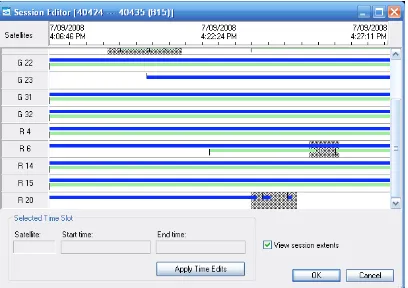
With the flexibility of post-processed static surveying, all of these testing issues can be resolved. As mentioned in section 2.4, GNSS post-processing software has the ability to freely toggle the use of specific satellites for each occupation in a solution. By producing a GNSS solution, then disabling the GLONASS satellites from the solution, a GPS-only solution can be formed. This removes the need for doubling up of equipment and trying to synchronise the start and finish times for two receivers at the same location. The observations will not only be able to be performed by the same make and model of antenna/receiver. It will in be the exact the same unit used for all observations in the occupations. Allowing the testing to be completed at the same time, place and with identical antennas and receivers.
2.7 Conclusions
Through extensive research and development from the instrument manufacturers, all compatibility and interoperability issues can be resolved without direct input of the user segment. Any future changes and possible issues with datums and signal access schemes could theoretically be resolved with firmware upgrades and minor (if at all) hardware upgrades).
for this reason can still be considered somewhat dated, with the recent advances in GNSS positioning technology. This can be observed by the document still referring only to the GPS constellation. However, the document does provide valid frameworks in which to perform GNSS surveys based on the GPS techniques outlined. Ultimately, the use of the same methodology of GPS surveys to perform GNSS surveys will determine if increased productivity and accuracy is achievable with the newer equipment. By providing a framework for manufacturers recommendations to predicate ICSM requirements, the document effectively becomes dynamic with the technological releases.
All of the standards and practices that are set out by the ICSM for GPS surveying have remained relatively unchanged since their inclusion in the document. These standards are based on GPS as the sole constellation being used, and running at a maximum of 24 satellites (FOC). However, with GPS running at 32 satellites and 12 extra satellites available for observation from the GLONASS constellation giving a total of 44 satellites, there is nearly the equivalent of two FOC constellations easily observable by anyone in the user segment with the right equipment.
CHAPTER 3 – TESTING METHODOLOGY
3.1 Introduction
The literature reviewed in Chapter 2 has indentified the fast static survey style as the method for testing in this research. Also analysed was the possible problems with GNSS compatibility, past testing methods and the removal of possible testing ambiguities to ensure the validity of this research.
This chapter will provide a detailed outline of the methods used to test hypothesises outlined in Chapter 1 based on the methods identified in Chapter 2. This will ensure that by using similar equipment and software or accessing the raw data that has been collected by this survey that the replication of the results produced by this research is possible.
For testing in Queensland, the standard practices used should not be different from those recommended by the ICSM and any major alterations would void the validity of the testing and its application to real world scenarios in Australia. To try to maintain the connection of this research to reality, the method used will essentially be identical to a typical static survey performed by any private practice and not anything requiring special testing facilities.
3.2 Testing Location Criteria
The six other stations have been determined by following criteria:
• At least four are to have First Order Horizontal Coordinates
• At least five are to have at least Fourth Order Vertical Levels
• The remaining two may or may not have any Horizontal or Vertical Information
• All are to be existing Permanent Marks in the NRW Survey Control Database (SCDB).
• All sites should be moderate to zero multipath for GNSS observations (where possible).
• Regular spacing (where possible) through the city centre of the Toowoomba and the surrounding suburbs with an area of about 10 square kilometres.
• Easily accessible by a two wheel drive vehicles.
• Easy to locate – a prominent feature.
3.3 Reconnaissance
One of the most important elements of geodetic surveying is planning. Formulating a mission plan will ensure that others have a much better understanding of what you are trying to achieve and how this objective is intended to be reached. In most cases (including this one) the surveyors whom are participating in the static survey will have had nothing to do with the project until the date of the survey.
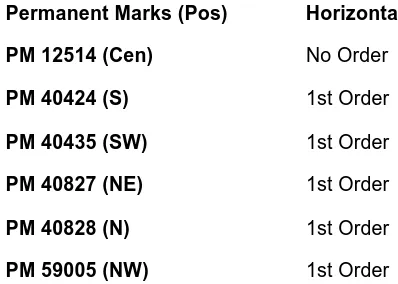
A list of 12 suitable marks was then compiled and their coordinates were uploaded into a Trimble Geo XT (mapping grade GPS seen in figure 3.1) for field inspection. The field inspection eliminated those difficult to find (including one trig station on top of a water tower at Picnic Point) and provided an opportunity to analyse the multipath potential of each location. Subsequently, the list was reduced to five PMs and an extra mark was selected nearby the centriod with “No Order” and “No Class” to increase the total number of PMs to six. A summary of the selected marks is in the table below and their mapped positions can be seen in Appendix Band full Form 6 Permanent Mark details in are Appendix C.
Figure 3.1 - Trimble Geo XT – Mapping Grade GPS
Permanent Marks (Pos) Horizontal Order Vertical Order
PM 12514 (Cen) No Order No Order
PM 40424 (S) 1st Order 4th Order
PM 40435 (SW) 1st Order 4th Order
PM 40827 (NE) 1st Order 4th Order
PM 40828 (N) 1st Order 4th Order
[image:36.595.115.314.84.226.2]PM 59005 (NW) 1st Order 4th Order
Table 3.1 - Selected Permanent Marks Order Details.
3.4 Equipment for Field Survey
The following equipment is available for utilisation in this research and will be used in the field survey:
• 1 x Trimble Net R5 Reference Station
• 1 x Trimble Zephyr Geodetic 2
• 3 x Trimble R8 GNSS Receivers
• 3 x TSC2 Data Collectors (running Trimble Survey Controller v12.22)
• 1 x Computer (Acting as data collector for the Net R5)
• 3 x Tripods
• 3 x Tribrachs
• 3 x Tribrach Adapters and Short Poles
• 3 x Offset Tapes
• 3 x Motor Vehicles
• 3 x Mobile Phones
3.4.1 Trimble GNSS Antennas and Receivers
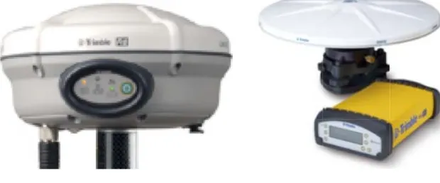
[image:37.595.183.493.333.462.2]Trimble antennas and receivers have been chosen for this study since the university currently only owns this brand of GNSS equipment (An SPS880 and a Net R5). To reduce complications and to follow the recommendation to have all receivers and antennas of the same make and model (USQ 2006), all three roving receivers will be Trimble R8 GNSSs. The SPS880 that was originally intended to be utilised but was not used for the survey since it had difficulty acquiring GLONASS satellites on the scheduled date of the mission. The GNSS equipment used for the survey is in figure 3.2.
Figure 3.2 - Trimble R8 GNSS and Net R5 with Zephyr Geodetic 2
(Source: Trimble Navigation Limited 2007a and 2007b)
All of the abovementioned receivers have the following common task specific features (Trimble Navigation Limited 2006 and 2007a and b):
• R-Track technology
• Claimed Fast Static accuracies:
o Horizontal±5mm + 0.5ppm RMS
o Vertical ±5mm + 1ppm RMS
• 72 channel tracking
• Custom GNSS chips
• Unfiltered, unsmoothed pseudo range measurements data for low noise, low multipath error, low time domain correlation and high dynamic response.
• Low elevation tracking technology
3.5 Mission Plan
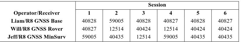
With the testing sites and the equipment all identified, the next step in the process is to formulate the mission plan. While forming a mission plan is not essential all static surveying, like surveys may only use a “base and rover” setup where only one baseline is measured per session. This survey, however, will use three roving receivers to measure two independent baselines per session and it will be necessary to plan the mission. To avoid two field parties arriving at the same mark for the same session, and to optimise the field time (normally the most expensive component) required for the entire survey and for many other logistical and geometrical reasons, the mission is planned.
Based on the testing sites, no baselines in the final solution will be longer than 10 kilometres as per the recommendation of the ICSM (2007) for fast static surveys. The quality of the survey to is aimed to produce Class A results since this is the highest level achievable by the Fast Static survey method. The ICSM recommends that surveys of high order be used mainly for scientific purposes. By choosing the highest class of survey possible for the fast static style, the results should be more revealing and any analogies between the GNSS and the GPS datasets should be more obvious and less prone to be caused by low quality of survey.
more than one baseline per session from the CORS data would produce trivial baselines). Although this step is not necessary, the data logged will be used more like a back up, in case of problems on station occupations and sessions. This data may also be used to replace a PM for the entire survey if it is found to be problematic.
With six stations, the requirement of three independent occupations for 20% of the stations and 100% of the stations to be occupied twice (ICSM 2007), it is mathematically possible to achieve this requisite in five sessions with three receivers. However, since things do not always run smoothly, an additional session will be added to ensure that extra sessions are not necessary on days after the scheduled mission date. Six sessions with three roving receivers will allow all of the stations to be independently occupied three times. If all things go to plan, and following the addition of CORS data, there should be a much higher than required amount of baselines and occupations to compute a tight 3-dimensional least squares network and additional baselines from the CORS data.
Now that all the information regarding the number of receivers and number of session was compiled, a baseline plan was then drafted (Appendix D). The plan aimed to minimise driving time while attempting to avoid having the same mark occupied consecutively in adjacent sessions.
Session Guides
Session
Operator/Receiver 1 2 3 4 5 6 Liam/R8 GNSS Base 40828 59005 40828 40827 40828 40827
Will/R8 GNSS Rover 40827 12514 40424 12514 40424 40424
Jeff/R8 GNSS MinSurv 59005 40435 12514 59005 40435 40435
Session
Station 1 2 3 4 5 6
40828 Liam Liam Liam
40827 Will Liam Liam
59005 Jeff Liam Jeff
12514 Will Jeff Will
40435 Jeff Jeff Jeff
40424 Will Will Will
Total Occupations
Permanent Mark Number
Session 40828 40827 59005 12514 40435 40424
1 1 1 1
2 1 1 1
3 1 1 1
4 1 1 1
5 1 1 1
6 1 1 1
[image:40.595.114.532.125.199.2]Total 3 3 3 3 3 3
Table 3.2 - Session Plan
3.6 Field Survey
The date of the survey was the Sunday the 7th of September 2008. The assisting surveyors were given the allocated GNSS equipment along with the necessary ancillary equipment. They were then given a briefing on the operation of the equipment and procedures to perform the fast static survey.
operating correctly, however the SPS880 was found to be unable to acquire GLONASS signals in all survey styles (Fast Static and RTK). It was also determined that university’s TSC2 was not running a recent enough version of Trimble Survey Controller (others were running v12.22) to be able to log GLONASS observations when in static mode. These issues with the SPS880 were critical, and therefore it was excluded from the survey and subsequently this research. Fortunately, I was able to contact a colleague in Toowoomba who had access to a R8 GNSS receiver and TSC2 also running Trimble Survey Controller 12.22, making all three roving receiver configurations identical. After successfully configuring and checking the new equipment, the survey was able to commence.
Each session in the survey followed the procedure as outlined below:
1. Drive to the PM allocated for the session (An example of two of the PMs sites in Figure 3.3 and 3.4).
2. Setup the R8 GNSS over the survey mark.
3. Measure the height of the antenna to the centre of bumper three times and enter the mean/median height into the controller.
4. The two assisting surveyors contacted me and once all field parties were ready, a “commence session” message was returned and the data logging was initiated. This was to ensure a complete overlap of data.
5. The session was ended after 20 minutes of data was recorded.
Figure 3.3 - R8 GNSS at PM 40435 in Session 2 – Worst Site for Sky Visibility.
[image:42.595.137.504.434.703.2]Despite the initial delays of starting the survey, the entire static mission was completed successfully in a single day. Immediately after the field survey concluded, the data from all the survey controllers/data recovered was transferred to a PC and several backups were made of that data. No post processing was carried out on the day of the survey.
3.7 Post Processing
This section is particularly important since many of the steps have been added to the regular procedures to allow for the GNSS and GPS comparisons. For this project, Trimble Business Centre Advanced (TBC) has seen selected as the software for post processing, since it can process GNSS baselines, perform least squares network adjustments and has advanced reporting functionality. In addition, since all of the GNSS hardware was of Trimble make, Trimble software should present the least compatibility issues.
3.7.1 Zero Constrained Adjustments
Figure 3.5 - Occupation Spreadsheet
The USQ CORS data was then accessed from the web interface at
http://www.usq.edu.au/engineer/surveying/gpsbase/local/liam.htm downloaded and imported into the TBC and all trivial baselines were removed (from the roving and CORS data). The CORS data was temporally disabled so that rover data could be analysed first.
Figure 3.6 - Baselines Processed and Network Adjusted
Figure 3.7 - Session Editor: GLONASS Satellites Disabled
Figure 3.8 - Session Editor: Filtering
The final set of results produced by a zero constrained adjustment was the “GPS Filtered” dataset. Similarly to how the GPS Raw results were produced, using the “GNSS Filtered” dataset and disabling the GLONASS satellites in the session editor the GPS Filtered results were produced after baseline processing and network adjustment.
3.7.2 CORS Data
Despite using only Trimble GNSS hardware and software for the survey, the data formats from the R8 GNSS receivers and the data from the Net R5 was different. The R8 GNSS output *.T01 files for its GNSS data and the Net R5 produced RINEX files. If time were available to debug this issue, the first effort to resolve this issue would be to attempt to convert all the files to the same format (i.e. all RINEX or *.T01) and reprocess the baselines. Next, may be to ensure all baselines are added and processed from the outset (and not disable initially as in this methodology).
3.7.3 Fully Constrained Adjustment
To verify the quality of both the Permanent Marks SCDB and the data collected by the Survey, MGA94 coordinates and AHD elevations of the known marks along with Ausgeoid98 was used to perform a fully constrained adjustment and compute the Local Uncertainties. The details of these marks can be seen in Appendix C. Since QA cannot be performed on the survey through terrestrial observations or EDM measurements due to a lack of line of sight between the marks, using known marks for the majority of the stations will allow QA to be completed through the comparison between the computed and the known coordinates via a fully constrained adjustment.
By individually toggling each remaining horizontal constraint and noting the network adjustment results, it was determined that statistically the best fit was produced by removing the horizontal constraint on PM 40435. Fortunately, this did not cause more geometric distortion than the removal of PM 59005 from the constraints. Finally, constraining both the horizontal and vertical by PM 59005 was tested with the new adjustment, which produced similar errors to when it was included the first time. PM 59005 was then removed from the adjustment. Figure 3.9 shows the final fully constrained network adjustment and its constraint configuration.
3.7.4 Decreasing the Length of Sessions
It was originally intended to make the precision comparisons of the filtered data with the network adjustment results. However, with the results of the GNSS and GPS filtered results being identical, the baseline processing report was the next point of comparisons. The difference between the baseline horizontal and vertical precisions averaged an improvement of about 0.001 metres for GNSS over GPS-only observations. The raw data was not included in this process, since in reality, unfiltered data would never be used for the final positions computed in a post processed geodetic survey.
Figure 3.10 - Removing Exactly 2 Minutes of Session Data
3.8 Conclusion
From the planning of the mission through to the post processing, all of the above procedures use the same methods that would be used to conduct static GPS network surveys in practice. Apart from the GNSS (rather than GPS) receivers used and the numerous extra stages of data processing required to produce the extra results necessary for this research, the above testing procedure conforms to the standards and best practices as recommended in SP1 by the ICSM and should be valid for use in Queensland and all of Australia.
practices) that have recently (in the last two years) purchased GNSS surveying equipment.
CHAPTER 4 – RESULTS
4.1 Introduction
All the procedures outlined in Chapter 3 have produced the required survey and statistical data through the report generation facilities of Trimble Business Centre. With all of the results complied, the data now needs to be presented graphically so any analogies in the data can be more easily identified.
The chapter will present a summary of the results generated in by Chapter 3 and found in Appendices G and F. This summary of data will be the information required to test the hypotheses outlined in section 1.3.1 and the information that surveyors would use from the survey.
This chapter will extract the information in the Baseline Processing Reports and Network Adjustment Reports from the aforementioned appendices. The data was extracted from the reports and the information, and then imported into Microsoft Excel for statistical analysis. The excel data was then imported into Apple’s Numbers to produce the graphs.
4.2 Zero Constrained Adjustments
The data in the graphs of this section is based on the calculated horizontal Positional Uncertainty as specified by the following equations (ICSM 2007):
Where:
q0 = 1.960790
q1 = 0.004071
q2= 0.114276
q3= 0.371625
And for vertical:
1.96 x (elevation error at 1)
Trimble Business Centre defaults to reporting the errors required at the 95% confidence level. Therefore, all of the data in the reports will need to be scaled back to the one-sigma level (i.e. scaled by the inverse of 1.96).
The class of the survey is determined by the technique used, the amount of occupations of each station and an empirically derived formula. With fast static as the method used and all the required amount of independent occupations exceeded, the highest achievable class of the survey is A (ICSM 2007). However, the Class that is achieved by indication of the statistical data will be assigned.
Where “d” is the distance to any station.
And “c” is an empirically derived number that assigns the class. The “c” values for some of the classes of survey follow:
Horizontal: Vertical:
3A = 2 3A = 2
2A = 8 2A = 6
4.2.1 GNSS Raw v GPS Raw
[image:55.595.141.475.202.519.2]The raw data GNSS raw and GPS raw that were produced in section 3.7.1 has been used to compute the positional uncertainties for every PM and the average has been computed are below in figures 4.1 and 4.2.
Figure 4.2 - Vertical Positional Uncertainty - GNSS Raw v GPS Raw
Raw GNSS Class Raw GPS Class PM Horizontal Vertical Horizontal Vertical 12514 2A 2A 2A 2A 40424 2A 2A 2A A 40435 2A 2A 2A A 40827 2A 2A 2A A 40828 2A 2A 2A 2A 59005 2A 2A 2A A
[image:56.595.140.433.482.598.2]4.2.2 GNSS Raw v GNSS and GPS Filtered
[image:57.595.144.434.275.577.2]The GNSS and the GPS filtered network adjustment results produced identical semi-major and semi-minor axes of their error ellipses. It was originally intended to only compare GNSS raw against GPS filtered positional uncertainty but since the two filtered results were the same, both will be compared. These results are in figures 4.3 and 4.4. The classes achieved for the filtered results are in section 4.5.
Figure 4.4 - Vertical Positional Uncertainty - Filtered GNSS/GPS v GNSS Raw
4.2.3 Filtered
Figure 4.5 - Horizontal Baseline Precision
[image:59.595.143.494.425.706.2]4.3 Productivity
For this section it was intended to remove one minute of data in every session, however, with the difference between the GNSS and GPS filtered data being smaller than expected, this required shortening the session lengths by 30 second at a time in order to gain more accurate results. The results remained unchanged until the two-minute mark was reached. To verify that the precisions reached were close to those reached with the GPS filtered data the differences between the baseline precisions were averaged. The average was 0.000m (for both horizontal and vertical) indicating that the precisions, while slightly different, were similar when all of the baselines were taken into account.
[image:60.595.124.479.450.713.2]By decreasing the lengths of the session by 30 seconds at a time, 30 seconds becomes the margin of error of the results. Inclusive of the error margin, with an average of 21 minutes per session and average maximum of two minutes for session length to be reduced, figure 4.7 was produced.
The extra processing time required in the office averaged only 10 seconds per baseline. As originally hypothesised, this extra post processing time is negligible and easily out weighed by the time saved in the fieldwork.
4.4 Fully Constrained Adjustment
The fully constrained adjustment was used as a form of quality assurance for this research, through connections to known high order PMs. The computation of local uncertainty and order are quantifies the fit of the observations to the local control network.
4.4.1 Local Uncertainty
Local uncertainty is calculated by the same formulae as positional uncertainty however; the error ellipse components are derived from a fully constrained adjustment (rather than a zero constrained adjustment). The results of the fully constrained adjustment preformed in section 3.7.3 can be seen in table 4.1. The constraints used in the adjustment are indicated by “Fixed” in the table.
Local Uncertainty
PM Horizontal Vertical
12514 0.009 0.015
40424 Fixed Fixed
40435 0.011 Fixed
40827 Fixed Fixed
40828 Fixed Fixed
[image:61.595.144.519.521.634.2]59005 0.013 0.027
4.4.2 Order of Survey
Order is a function of class, the quality of the fit to the local marks and the quality of the marks coordinates. As with local uncertainty, is the result of a fully constrained adjustment with one caveat, no mark can have an order above the order of the mark in which it was derived.
Order
PM Horizontal Vertical 12514 1st 4th
[image:62.595.145.519.215.336.2]40424 1st 4th 40435 1st 4th 40827 1st 4th 40828 1st 4th 59005 1st 4th
Table 4.3 - Order Assigned to PMs (GNSS Filtered)
4.5 NRW Form 6 Information
Horizontal
PM Datum Latitude Longitude Easting Northing 12514 GDA94 S27°33'52.55197" E151°56'58.95191" 396317.287 6950588.058 40424 GDA94 S27°36'37.83052" E151°56'04.22078" 394860.174 6945489.266 40435 GDA94 S27°35'05.85884" E151°55'46.48617" 394349.533 6948315.233 40827 GDA94 S27°32'56.66936" E151°59'35.40740" 400593.839 6952343.303 40828 GDA94 S27°32'10.37535" E151°57'09.72110" 396586.030 6953734.721 59005 GDA94 S27°33'01.25973" E151°54'10.16304" 391674.508 6952126.284
MGA94: Zone 56 Vertical
PM Datum Height 12514 AHD D 593.542
[image:63.595.110.410.379.622.2]40424 AHD 683.293 40435 AHD 682.050 40827 AHD 614.622 40828 AHD 608.797 59005 AHD D 615.137
Table 4.4 - Survey Coordinate Information
Local Uncertainty Positional Uncertainty PM Horizontal Vertical Horizontal Vertical 12514 0.009 0.015 0.005 0.009 40424 Fixed Fixed 0.008 0.011 40435 0.011 Fixed 0.006 0.010 40827 Fixed Fixed 0.007 0.011 40828 Fixed Fixed 0.005 0.008 59005 0.013 0.027 0.006 0.012
Order Class
PM Horizontal Vertical Horizontal Vertical 12514 1st 4th 3A 2A 40424 1st 4th 2A 2A 40435 1st 4th 3A 2A 40827 1st 4th 2A 2A 40828 1st 4th 3A 2A 59005 1st 4th 3A 2A
4.6 Conclusion
CHAPTER 5 – DATA ANALYSIS
5.1 Introduction
With all the data extracted from the baseline processing reports and the network adjustment reports required to address the aims of the research complied in Chapter 4,this chapter will analyse the data.
Chapter 5 will critically analyse the results generated in Chapter 4. This analysis will investigate the improvements in precision and productivity that GNSS has made over GPS. The magnitude of these gains will be analysed in order to determine their relationship to real word benefits to the end users – surveyors.
Figure 5.1 - Combined Horizontal Positional Uncertainties
[image:66.595.121.403.440.687.2]5.2 Raw - GNSS v GPS
At any one time, the GNSS data had three to five extra GLONASS satellites from which to observe extra raw data. In any occupation, this translated to recording 25 to 35 percent more data. GNSS raw data shows an improved positional uncertainty over GPS raw data by an average of 33% in horizontal results and an average of 26% for the vertical.
It would appear that the site with the optimal sky visibility has gained the most from the additional data (refer to figure 51 and 5.2, PM 40424 has the best sky visibility). Given that much other research has proven that RTK GNSS is more reliable than RTK GPS in areas of high multipath, this result was unexpected. It can be rationalised that the best sites for GNSS surveying will improve the most since minimal noisy data is being observed with extra quality data. While sites that are less than optimal for GNSS surveying may benefit from observing extra clean data, extra noisy data is also observed. However, despite having observed extra noisy data, the consistent improvement in precision of GNSS over GPS suggests that the extra clean data outweighs the noisy data.
5.3 GNSS Raw v Filtered
As mentioned in section 4.2.2, the GNSS and GPS filtered results were identical. By having identical results, the comparisons will be made to both the filtered results against the GNSS raw results. While it can be seen in figures 5.1 and 5.2 that GNSS raw data have had significant gains over GPS raw data, GNSS raw data has still not made it to the quality level of filtered data.
towards the precision of filtered data. Until more satellites come online, there is no substitute for the filtering process that is part of post processing.
5.4 Filtered - GNSS v GPS
The hypothesis reflects that the GNSS filtered was expected to make some gains over GPS filtered. The direct comparison between the filtered GNSS and GPS baseline reports suggest that GNSS was in some cases equal to, but in most cases better than the GPS baseline precision.
While there were precision gains made in the baseline processing reports, the network adjustment reports suggest that the gains made do not add to the overall result of the zero constrained adjustment. Further testing may be required to prove or disprove this hypothesis; therefore the testing in this research regarding the improvement of precision of GNSS filtered results over GPS filtered results is inconclusive.
5.5 Productivity