Anomalous diffusion with linear reaction dynamics: From
continuous time random walks to fractional reaction-diffusion
equations
B.I. Henry∗ and T.A.M. Langlands†
Department of Applied Mathematics, School of Mathematics, University of New South Wales, Sydney NSW 2052, Australia.
S.L. Wearne‡
Center for Biomathematical Sciences,
Abstract
We have revisited the problem of anomalously diffusing species, modelled at the mesoscopic level
using continuous time random walks, to include linear reaction dynamics.
If a constant proportion of walkers are added or removed instantaneously at the start of each
step then the long time asymptotic limit yields a fractional reaction-diffusion equation with a
fractional order temporal derivative operating on both the standard diffusion term and a linear
reaction kinetics term. If the walkers are added or removed at a constant per capita rate during
the waiting time between steps then the long time asymptotic limit has a standard linear reaction
kinetics term but a fractional order temporal derivative operating on a non-standard diffusion term.
Results from the above two models are compared with a phenomenological model with standard
linear reaction kinetics and a fractional order temporal derivative operating on a standard diffusion
term.
We have also developed further extensions of the CTRW model to include more general reaction
dynamics.
PACS numbers: 05.40.-a,05.60.Cd,82.40.Ck,82.39.Rt,89.75.Kd
∗Electronic address: [email protected]
†Electronic address: [email protected]
‡Electronic address: [email protected]; Also at Fishberg Department of Neuroscience.;
I. INTRODUCTION
Reaction-diffusion equations have been studied extensively as mathematical models of systems with reactions and diffusion across a wide range of applications including; nerve cell signalling, animal coat patterns, population dispersal, and chemical waves. The generic form of these equations is [1]
∂n(x, t)
∂t =D∇
2n(x, t) +f(n(x, t)) (1)
wherenis a vector whose components represent the numbers of a particular species per unit volume. The first term on the right hand side accounts for the spatial diffusion of the species and D is a diagonal matrix whose elements are the diffusivities of the different species. The second term on the right hand side, a functional of n, accounts for ‘reactions’ that produce or destroy species. This partial differential equation can be motivated by a mesoscopic description based on a coarse grained representation of space with diffusion between cells and reactions within cells [1]. The cells are considered to be arbitrarily small so that the diffusion of reactants within cells is instantaneous. In this case the reactants within cells are homogeously mixed and the production or destruction of particles in the cells is a reaction-limited process that can be modelled according to the law of mass action. The characteristic length scale `D and time scale τD for the mesoscopic description are defined relative to the following physical scales: the characteristic size of a reaction zone δ`R; the characteristic microscopic diffusion time for encounters between reactants δτD; the microscopic reaction time δτR; the size of the domain L; the time scale of the experiment T. Explicitly (i)
δ`R `D L and (ii) δτD δτR τD T. The length scale `D and the time scale τD are both considered to be arbitrarily small but (in the case of standard Brownian motion) `2
D/τD is finite.
Faster than linear scaling (α > 1) is referred to as super-diffusion and slower than linear scaling (0< α <1) is referred to as sub-diffusion. In recent years the additional motivation for these studies has been stimulated by experimental measurements of sub-diffusion in porous media [5], glass forming materials [6], biological media [7, 8], and Monte Carlo studies of sub-diffusion in materials with trapping or binding sites [9]. One of the most successful theoretical paradigms to emerge from this research has been fractional calculus models for anomalous diffusion justified at a mesoscopic level by Continuous Time Random Walks (CTRWs) [3, 4, 10]. In the CTRW model anomalous sub-diffusion arises when the asymptotic long time limit of the waiting time probability density function is heavy tailed, ie., ψ(t) ∼ t−α−1 with 0 < α < 1. The evolution equation for the concentration of
non-reacting species undergoing sub-diffusion can then be modelled using a fractional diffusion equation which differs from the conventional diffusion equation in that it has a fractional order temporal derivative acting on the spatial Laplacian.
hoc. Very recently, Sokolov, Schmidt and Sagu´es [25] revisted the problem of reactions with sub-diffusion, and in the case of a monomolecular conversion A → B, they found that the fractional reaction-diffusion equation includes the effects of the reactions in both an additive reaction term and a non-standard diffusion term. The latter can not be represented by a temporal fractional order derivative operating on a standard diffusion term.
Here we have revisited the CTRW model to allow for the addition or removal of species via one of three different linear processes: (i) Walkers are added or removed via a source/sink term with linear reaction rate kinetics in the generalized CTRW model introduced by Henry and Wearne [11]. The long time asymptotic limit is a fractional reaction-diffusion equation with standard linear reaction kinetics and a fractional order temporal derivative operating on a standard diffusion term. (ii) A constant proportion of walkers is added or removed instaneously at the start of each step. In this case the long time asymptotic description in terms of fractional reaction-diffusion equations yields a fractional order temporal derivative operating on both the diffusion term and a linear reaction kinetics term. (iii) Walkers are added or removed at a constant per capita rate during the waiting time before a step is made. Here the long time asymptotic limit in terms of fractional reaction-diffusion equations can be represented with standard linear reaction kinetics but a fractional order temporal derivative operating on a non-standard diffusion term.
A sub-diffusive CTRW model for case (ii) with a linear degradation term was considered recently by Hornung, Berkowitz and Barkai [26]. Here we have formulated the CTRW in terms of a fractional diffusion equation with a fractional order temporal derivative operating on both the (Laplacian) diffusion term and the (linear) reaction term. In case (iii) we obtain similar CTRW results to those recently reported by Sokolov, Schmidt and Sagu´es [25] but we have represented the long time asymptotics by a fractional reaction diffusion equation with a linear reaction term and a temporal order fractional derivative operating on a non-standard diffusion term.
We have obtained explicit solutions for the three fractional reaction-diffusion equations considered in these models. The different solutions are informative of different physical processes involving anomalous diffusion with linear reaction dynamics.
subsequent extension to include source and sink terms. In section III we introduce linear reaction dynamics into the CTRW formalism according to the different processes outlined above and we derive the appropriate fractional reaction-diffusion equations for the long time asymptotic behaviour. In section IV we outline further extensions of the CTRW model to include more general reaction dynamics. In section V we present explicit solutions of the fractional reaction-diffusion equations resulting from the different linear models. In section VI we discuss the results.
II. CONTINUOUS TIME RANDOM WALKS
The continuous time random walk (CTRW) was introduced by Montroll and Weiss [27], and Scher and Lax [28], as a generalization of the standard random walk introduced by Pearson in 1905 [29]. In Pearson’s formulation the random walk consists of a sequence of equal length steps taken at regular time intervals. In the CTRW the waiting times between successive steps and the length of the steps are both random variables with the associated probability density Ψ(x, t) for the particle to step a distance x after waiting a time t. In the original formulation by Montroll and Weiss [27] the walk was considered to have taken place on a discrete lattice.
A fundamental quantity to calculate is the conditional probability density p(x, t|x0,0)
that a walker starting from position x0 at time t = 0 is at position x at time t. First it is
useful to consider the conditional probability density qn(x, t|x0,0) that a walker starting at
x0 at time zero arrives at position x at time t after n steps. This latter probability density
satisfies the recursion equation [28]
qn+1(x, t|x0,0) =
X
x0
Z t
0
Ψ(x−x0, t−t0)qn(x0, t0|x0,0)dt0 (2)
where Ψ(x−x0, t
−t0) is the probability density that a random walker jumps a distance x−x0 after waiting a time t
−t0 in a single step. Note that the sum over x0 includes the possibility x0 =x. The initial condition that the walker is at x
0 at time zero,
q0(x, t|x0,0) =δx,x0δ(t), (3)
satisfies the normalization
X
x0
Z ∞
0
The conditional probability density q(x, t|x0,0) that a walker arrives at position xat time t
after any number of steps is given by
q(x, t|x0,0) =
∞
X
n=0
qn(x, t|x0,0). (5)
Note that we can write ∞
X
n=0
qn(x, t|x0,0) =q0(x, t|x0,0) +
∞
X
n=0
qn+1(x, t|x0,0),
so that, after performing a summation overn, the recursion relation, Eq.(2), can be written as [28, 30]
q(x, t|x0,0) =
X
x0
Z t
0
Ψ(x0, t0)q(x−x0, t−t0|x0,0)dt0+δ(t)δx,x0. (6)
In the remainder it is supposed that the probability density Ψ(x, t) decouples in space and time, i.e.,
Ψ(x, t) =ψ(t)λ(x) (7)
where ψ(t) is the waiting time probability density given by
ψ(t) =X x0
Ψ(x0, t) (8)
and λ(x) is the step length probability density given by
λ(x) =
Z ∞
0
Ψ(x, t0)dt0. (9)
It is also useful to define the survival probability distribution Φ(t) that the walker does not take a step in time intervalt
Φ(t) = 1−
Z t
0
ψ(t0)dt0 =
Z ∞
t
ψ(t0)dt0. (10)
The conditional probability density p(x, t|x0,0) that a walker starting from the origin at
time zero is at position x at time t is equivalent to the probability density that the walker arrived at x at any earlier time t0 and thereafter did not take a step, i.e., [27, 28, 30]
p(x, t|x0,0) =
Z t
0
q(x, t−t0
The results in Eq.(6) and Eq.(11) can be combined using Laplace transforms to yield the master equation for the probability density p(x, t|x0,0). The Laplace transform of Eq.(11)
yields
ˆ
p(x, u|x0,0) = ˆq(x, u|x0,0) ˆΦ(u), (12)
and the Laplace transform of Eq.(6) yields
ˆ
q(x, u|x0,0) =
X
x0 ˆ
Ψ(x0, u)ˆq(x−x0, u|x0,0) +δx,x0. (13)
We can combine these two results to obtain
ˆ
p(x, u|x0,0) =
X
x0 ˆ
Ψ(x0, u) ˆΦ(u)ˆq(x−x0, u|x0,0) + ˆΦ(u)δx,x0,
= X
x0 ˆ
Ψ(x0, u)ˆp(x−x0, u|x0,0) + ˆΦ(u)δx,x0. (14)
The inverse Laplace transform of Eq.(14) now yields the master equation [30];
p(x, t|x0,0) = Φ(t)δx,x0 +
X
x0
Z t
0
p(x0, t0
|x0,0)Ψ(x−x0, t−t0)dt0. (15)
Most of the recent literature on CTRWs take Eq.(15), or the continuum version [31]
p(x, t|x0,0) = Φ(t)δx,x0 +
Z t
0
ψ(t−t0)
Z ∞
−∞
λ(x−x0)p(x0, t0
|x0,0)dx0
dt0. (16)
as the starting point for further analysis. For example Mainardi and co-workers [31] motivate this equation on probability arguments with the interpretation that the first term expresses the persistence of a walker at the initial position and the second term is the contribution from a walker being at point x0 at time t0 and then jumping to x and t after waiting a time t−t0.
It follows from Eq.(15), that if there is an initial concentration of c(x0,0|x0,0) random
walkers at x = x0 at time t = 0 and if these walkers do not interact then the expected
concentration c(x, t|x0,0) at position x and time t is given by
c(x, t|x0,0)
c(x0,0|x0,0)
= Φ(t)δx,x0 +
X
x0
Z t
0
c(x0, t0 |x0,0)
c(x0,0|x0,0)
Ψ(x−x0, t
−t0)dt0. (17)
After multiplying by the initial concentration we have
c(x, t|x0,0) = Φ(t)c(x0,0|x0,0)δx,x0+
X
x0
Z t
0
c(x0, t0
Now suppose that we have a different initial concentration at each possible starting point x0 and sum over all possible starting points then
X
x0
c(x, t|x0,0) =
X
x0
Φ(t)c(x0,0|x0,0)δx,x0
+X
x0
Z t
0
X
x0
c(x0, t0|x0,0)Ψ(x−x0, t−t0)dt0 (19)
= Φ(t)c(x,0|x,0) +X x0
Z t
0
X
x0
c(x0, t0
|x0,0)Ψ(x−x0, t−t0)dt0. (20)
We now identify the number density
n(x, t) =X x0
c(x, t|x0,0) (21)
as the total expected concentration of walkers at positionxand time t(independent of their starting locations) and
n(x,0) =c(x,0|x,0) (22)
as the initial concentration of walkers atx. The result in Eq.(20) can now be written as
n(x, t) = Φ(t)n(x,0) +X x0
Z t
0
n(x0, t0)Ψ(x−x0, t−t0)dt0. (23)
III. CONTINUOUS TIME RANDOM WALKS WITH SUB-DIFFUSION AND
LINEAR REACTION KINETICS
In earlier work [11] we considered an extension of the conservation equation, Eq.(23) to incorporate sources and sinks as follows;
n(x, t) = Φ(t)n(x,0) +X x0
Z t
0
n(x0, t0)Ψ(x−x0, t−t0)dt0+
Z t
0
Φ(t−t0)s(x, t0)dt0. (24)
The heuristic interpretation of the additional source/sink term was that it represents the net contribution to the concentration of walkers at x and t due to i) walkers added at x at time t0 < t that then do not jump from x over the time (t
kinetics from the law of mass action. However the resulting phenomenological model has not been justified at the mesoscopic level of the random walks and the physical interpretation is not clear. Nevertheless one of the appealing features of this model is that the asymptotic long time limit yields a fractional reaction-diffusion equation [11] that only differs from the standard reaction-diffusion equation through a fractional temporal order derivative operating on the standard spatial Laplacian. This model can thus be derived phenomenologically from the standard conservation law for reaction-diffusion processes [32] by replacing the general flux transport with a fractional temporal order derivative operating on the gradient of the concentration - a time fractional Fickian process [33]. Similarly the space fractional diffusion equation [34] can be reconciled with a space fractional Fickian process [35]. In the models below we have attempted to move beyond a phenomenological description by incorporating the physical basis of the source/sink terms at the level of the random walks.
A. Instantaneous creation and annihilation processes
In this subsection we consider a simple extension of the standard CTRW model to include the instantaneous addition or removal of a fixed proportion of the walkers at the start of the waiting time before they take their next step. A sub-diffusive CTRW formulation of this problem in the case of removals (physically representing the degradation of morphogens) was considered recently by Hornung, Berkowitz and Barkai [26]. In the derivation below we show that the CTRW for this problem can be formulated as a fractional reaction-diffusion equation. One of the appealing features of this representation is that it provides a ready comparison between standard reaction-diffusion equations and the corresponding problem with anomalous diffusion. Another appealing feature is that standard mathematical methods for partial differential equations and the mathematical tools of fractional calculus can be employed to provide the asymptotic long time behaviour of this problem without further approximation.
The probability density for walkers to arrive at position x at time t at the end of their (n+ 1) th step, given that a fixed proportion are added or removed instantaneously (at the start or end of the step), is now given by
qn+1(x, t) =
Z t
0
X
x0
Here we have increased (+) or reduced (−) the walkers that arrived after n steps by a constant proportion k ∈(0,1). We could of course write r= (1±k) and then
qn+1(x, t) =r
Z t
0
X
x0
qn(x0, t0)ψ(t−t0)λ(x−x0)dt0. (26)
Similar to Eq.(6) we can now sum over n to obtain
q(x, t) =rX
x0
Z t
0
ψ(t−t0)λ(x−x0)q(x0, t0)dt0+δ(t)δx,x0 (27)
where we have included the initial condition that walkers are starting at x0.
We now consider the probability density for walkers to be at x at time t. This is given by
p(x, t) =r
Z t
0
Φ(t−t0)q(x, t0)dt0, (28)
i.e., the walkers at x at time t are those that arrived there at an earlier time t < t0 and then did not jump away, increased or reduced by the constant fraction of arrivals that were added or removed by the source/sink term. Note that in the caser = 1−k, Eq.(28) can be written as [26]
p(x, t) =
Z t
0
Π(t−t0)q(x, t0)dt0 (29)
with
Π(t) = 1−(1−k)
Z t
0
ψ(t0)dt0−k
Z t
0
ψR(t0)dt0 (30)
and ψR(t) =δ(t). In this representation, ψR(t) is a degradation time density (taken to be instantateous here) and k can be considered as the probability for degradation to occur, so that Π(t) is the probability that the walker survives at position x and does not degrade during the time interval t.
It follows from Eq.(27) that we can also write
p(x, t) =r
Z t
0
Φ(t−t0)δ
x,x0δ(t0)dt0+r2
Z t
0
Φ(t−t0) X
x0
Z t0
0
ψ(t0
−t00)λ(x
−x0)q(x0, t00)dt00
!
dt0
(31) We can combine the results of Eq.(28) and Eq.(31) as in the derivation of the master equa-tion, Eq.(15), to obtain
p(x, t) =rΦ(t)δx,x0 +r
X
x0
Z t
0
p(x0, t0)ψ(t
−t0)λ(x
Allowing for walkers starting from different initial positions and proceeding through steps similar to those leading to Eq.(23) we have the following equation for the number density
n(x, t) =rΦ(t)n(x,0) +rX
x0
Z t
0
n(x0, t0)ψ(t
−t0)λ(x
−x0)dt0. (33)
The fractional reaction diffusion equation in Henry and Wearne [11] was derived after a spatial Fourier transform and temporal Laplace transform of the master equation, Eq.(24), with asymptotic expansions for small values of the Fourier and Laplace variables, followed by inverse transforms using the definition of the Riemann-Liouville fractional derivative. We follow this approach here starting with the new balance equation, Eq.(33). The Fourier-Laplace transform of Eq.(33) with Fourier variable q and Laplace variableu yields
ˆˆ
n(q, u) =rΦ(ˆ u)ˆn(q,0) +rψˆ(u)ˆλ(q)ˆˆn(q, u) (34)
The Laplace transform of the survival probability, Eq.(10), can be written as
ˆ
Φ(u) = 1 u −
ˆ ψ(u)
u (35)
and the small q asymptotic expansion of the step length density is given by
ˆ
λ(q)∼1− q
2σ2
2 +O(q
4) (36)
with
σ2 =
Z
r2λ(r)dr (37)
finite. We can thus approximate Eq.(34) as
uˆˆn(q, u) =r1−ψˆ(u)nˆ(q,0) +ruψˆ(u)
1−q
2σ2
2
ˆˆ
n(q, u). (38)
We now consider asymptotic small u results for a heavy tailed waiting time density
ψ(t)∼ κ τD
t τD
−α−1
(39)
that is characteristic of anomalous sub-diffusion (see e.g., [3]). In this expression K is a dimensionless constant and τD is the characteristic mesoscopic time scale. The asymptotic Laplace transform for this density function is obtained from a Tauberian (Abelian) theorem [36, 37] as
ˆ
ψ(u)∼1− κΓ(1−α)
α τ
α
The asymptotic results in Eqs.(39),(40) apply for times t τD. We now substitute the above expansion into Eq.(38) to arrive at
unˆˆ(q, u) = rκΓ(1−α)
α τ
α
Duαnˆ(q,0) +ru
1−κΓ(1−α)
α τ
α
Duα 1−
q2σ2
2
ˆˆ
n(q, u) (41)
If we re-arrange this equation and retain only leading order terms then
unˆˆ(q, u)−nˆ(q,0) =− α κΓ(1−α)τα
D
u1−α
1−r
r nˆˆ(q, u) + q2σ2
2 ˆˆn(q, u)
. (42)
The above equation can also be derived without long time asymptotics in the special case where the waiting time density is given by the derivative of a Mittag-Leffler function [38]. The inverse Laplace transform and inverse Fourier transform of Eq.(42) now yields
∂n
∂t =D(α)D
1−α∂2n
∂x2 +
α κΓ(1−α)τα
D
r−1 r
D1−αn (43)
where the diffusivity
D(α) = σ
2α
2κΓ(1−α)τα D
(44)
and we use the notation
D1−α[y(x, t)] = ∂1
−α
∂t1−αy(x, t) +L
−1
{∂ −α
∂t−αy(x, t)|t=0}, 0< α <1 (45) where
∂1−α
∂t1−αy(x, t) (46)
is the Riemann-Liouville fractional derivative defined as the ordinary derivative of the Riemann-Liouville fractional integral
D−α[y(x, t)] = ∂ −α
∂t−αy(x, t) = 1 Γ(α)
Z t
0
y(x, t)
(t−s)1−αds, 0< α <1. (47) Note that the operator Dγ has a different definition depending on whether γ is positive, Eq.(45), or negative, Eq.(47) (see Appendix A). Note too that the inverse Laplace transform of the fractional integral evaluated at time zero, which appears in the operator D1−α in Eq.(45), will cancel in Eq.(43) if the method of Laplace transforms is applied to find the solution.
consistent with Eq.(10) in [26]. However after representing Eq.(40) by a fractional reaction-diffusion equation in Eq.(43) we can find an explicit solution in this space-time domain without further approximation (see Section V.). By comparison, the authors of [26] obtain an approximate space-time representation of Eq.(10) (see section IV of [39]).
B. Non-instantaneous creation and annihilation processes
We now consider an extension of the CTRW model to include the addition or removal of walkers at a constant per capita rate during the times that they wait before taking their next step. The CTRW model in this case is similar to that recently formulated [25] for monomolecular conversions. The probability density for arrivals at the end of the (n+ 1)th step in this case is given by
qn+1(x, t) =
Z t
0
X
x0
qn(x0, t0)e±k(t−t 0)
ψ(t−t0)λ(x−x0)dt0. (48)
The exponential factor accounts for the constant per capita increase (+) or decrease (−) during time intervals t−t0. In the usual way after summing over n we have
q(x, t) = X x0
Z t
0
ψ(t−t0)λ(x
−x0)q(x0, t0)e±k(t−t0)
dt0+δ(t)δ
x,x0 (49)
The probability for walkers to be atx at time t is now given by
p(x, t) =
Z t
0
Φ(t−t0)q(x, t0)e±k(t−t0)dt0 (50)
=
Z t
0
Φ(t−t0)e±k(t−t0) X x0
Z t0
0
ψ(t0
−t00)λ(x
−x0)q(x0, t00)e±k(t0−t00) dt00
!
dt0
+
Z t
Φ(t−t0)e±k(t−t0)
δx,x0δ(t0)dt0 (51)
= Φ(t)e±ktδx,x0 +
X
x0
Z t
0
p(x0, t0)e±k(t−t0)ψ(t−t0)λ(x−x0)dt0. (52)
The concentration balance equation in this case is
n(x, t) = Φ(t)e±ktn(x,0) +X x0
Z t
0
n(x0, t0)e±k(t−t0)
ψ(t−t0)λ(x
−x0)dt0. (53)
and the Fourier-Laplace transform of the balance equation results in
ˆˆ
From the result in Eq.(35) we can re-write the above equation as
(u∓k)ˆˆn(q, u) = 1−ψˆ(u∓k)nˆ(q,0) + (u∓k)ˆλ(q) ˆψ(u∓k)ˆˆn(q, u). (55)
In the case of anomalous sub-diffusion we use the asymptotic results in Eq.(36) and Eq.(40) to obtain
unˆˆ(q, u)−nˆ(q,0) =− α κΓ(1−α)τα
D
(u∓k)1−αq2σ2
2 nˆˆ(q, u)±knˆˆ(q, u) (56)
and then after taking the inverse Fourier and Laplace transforms,
∂n(x, t) ∂t =L
−1
{D(α)(u∓k)1−α∂
2nˆ(x, u)
∂x2 } ±kn(x, t) (57)
where it remains to evaluate the inverse Laplace transform represented by the operator L−1{}. This step follows from the identity
L−1{u1−αyˆ(u)}=D1−αy(t) (58)
together with the shift theorem
L−1
{z(u±k)}=e∓ktz(t) (59)
so that finally we have
∂n ∂t =e
±kt
D(α)D1−α
e∓kt∂
2n
∂x2
±kn (60)
We note in passing that we can use Leibniz’s formula extended to fractional derivatives [40] to re-write the above equation as
∂n ∂t =e
±ktD(α)
∞
X
j=0
1−α
j
Dje∓kt
D1−α−j∂2n
∂x2
±kn (61)
or equivalently
∂n
∂t = D(α)
D1−α∂2n
∂x2
±kn
+D(α) ∞
X
j=0
Γ(2−α)
Γ(1−α−j)(j+ 1)!(∓k) j+1
D−α−j∂
2n
∂x2
IV. CONTINUOUS TIME RANDOM WALKS WITH SUB-DIFFUSION AND GENERAL REACTION KINETICS
A. Instantaneous creation and annihilation processes
In this subsection we consider arbitrary reaction kinetics coupled with the CTRW model to include the instantaneous addition or removal of walkers at the start of the waiting times between steps. The general equation for the density for walkers to arrive at position x at time t at the end of their (n+ 1)th step in this case can be written
qn+1(x, t) =
Z t
0
X
x0
(qn(x0, t0) +sn(x0, t0))ψ(t−t0)λ(x−x0)dt0. (63)
where sn(x, t) is the density for walkers that are added and/or removed at the start of the waiting time for the (n+ 1)th step.
If we identify s(x, t) =P∞n=0sn(x, t) then the arrival density is given by
q(x, t) =X x0
Z t
0
ψ(t−t0)λ(x−x0) (q(x0, t0) +s(x0, t0)) dt0+δ(t)δx,x0. (64)
The density for a random walker to be at x at timet is now
p(x, t) =
Z t
0
Φ(t−t0) (q(x, t0) +s(x, t0))dt0 (65)
and the balance equation for the concentration of walkers atx and t becomes
n(x, t) = Φ(t)n(x0, t) +
X
x0
Z t
0
ψ(t−t0)λ(x
−x0)n(x0, t0)dt0+
Z t
0
Φ(t−t0)s(x, t0)dt0. (66)
The asymptotic long time behaviour is then governed by the non-homogeneous fractional diffusion equation
∂n
∂t =D(α)D
1−α
∂2n
∂x2
+s(x, t) (67)
The above balance equation, Eq.(66), leading to the non-homogeneous fractional diffusion equation, Eq.(67), was motivated by heuristic arguments in [11]. We could consider these equations with any source or sink term for s(x, t) including reaction terms
s(x, t) =f(n(x, t)) (68)
but the physical interpretation of this is not clear. For example in the case of linear reaction dynamics f(n(x, t) =±kn(x, t) we have
∂n
∂t =D(α)D
1−α
∂2n
∂x2
but this does not equate with the fractional reaction diffusion equation, Eq.(43), correspond-ing to the CTRW model with linear reaction dynamicss(x, t) =P∞n=0±kqn(x, t) =±kq(x, t) that we considered in section III A. To further highlight the difference between the two models it is useful to compare the balance equations directly. Note that we can re-write the balance equation, Eq.(33), as
n(x, t) = Φ(t)n(x,0) +X x0
Z t
0
ψ(t−t0)λ(x
−x0)n(x0, t0)dt0+r−1
r n(x, t). (70)
Thus the source term s(x, t) in the general balance equation, Eq.(66), corresponding to this model is given by equating
Z t
0
Φ(t−t0)s(x, t0)dt0 = r−1
r n(x, t). (71)
It is a simple matter to solve this equation for s(x, t) by the method of Laplace transforms. Explicitly we have
ˆ
s(x, u) = r−1 r
ˆ n(x, u)
ˆ
Φ(u) (72)
and then after using the asymptotic results in, Eqs.(35),(40) we have
s(x, t) = r−1 r
α κΓ(1−α)τα
D
D1−αn, (73)
so that Eq.(43) is again seen as a special case of Eq.(67).
B. Non-instantaneous creation and annihilation processes
In this subsection we consider arbitrary time dependent creation and annihilation pro-cesses coupled with the CTRW model to include the non-instantaneous addition or removal of walkers during the waiting times between steps. There are two generalizations as follows:
1. General linear model
the balance equation can be written as
n(x, t) = Φ(t)f(t)n(x,0) +X x0
t
Z
0
n(x0, t0)ψ(t−t0)λ(x−x0)f(t−t0)dt0. (74)
Taking the Fourier-Laplace transform of Eq. (74) and using Eq. (36) we find
bb
n(q, u) (1− L {ψ(t)f(t)}(u)) =L {Φ(t)f(t)}(u)bn(q,0)
−q2σ
2
2 L {ψ(t)f(t)}(u)bbn(q, u). (75)
This equation can be simplified by exploiting relationships between the transforms L {Φ(t)f(t)}(u) and L {ψ(t)f(t)}(u). First we note
d
dt (Φ(t)f(t)) =−ψ(t)f(t) +f
0(t)Φ(t) (76)
where we have used the identity
dΦ dt =
d dt
∞
Z
t
ψ(t0)dt0
=−ψ(t). (77)
Now taking the Laplace transform of Eq. (76) we find
uL {Φ(t)f(t)}(u)−Φ(0)f(0) =−L {ψ(t)f(t)}(u) +L {Φ(t)f0(t)
}(u) (78)
or
−L {ψ(t)f(t)}(u) =uL {Φ(t)f(t)}(u)−f(0)− L {Φ(t)f0(t)
}(u) (79)
noting Φ(0) = 1. Eq. (75) then becomes after some manipulation and inverting the Fourier transform
L
∂n ∂t
(u) = σ
2
2
L {ψ(t)f(t)}(u) L {Φ(t)f(t)}(u)
∂2nb
∂x2 +
L {Φ(t)f0(t)
}(u) +f(0)−1
L {Φ(t)f(t)}(u) bn. (80)
To simplify further requires detailed information about the small u behaviour of the three transforms L {Φ(t)f(t)}(u), L {ψ(t)f(t)}(u), and L {Φ(t)f0(t)
}(u). In the case of f(t) =ekt, the coefficient of
b
2. General reaction-kinetics model
We finally consider the extension of the CTRW model for general reaction-kinetic equa-tions for reacequa-tions between the end of the nth step and the end of the (n + 1)th step, i.e.,
∂qn
∂t =f(qn). (81)
In this general case we can integrate over the time interval t−t0 to write the arrival density after the (n+ 1)th step as
qn+1(x, t) =
Z t
0
X
x0
F−1(F(qn(x, t0)) + (t−t0))ψ(t−t0)λ(x−x0)dt0 (82)
where
F0(q
n) = 1 f(qn)
. (83)
We can also write
p(x, t) =
Z t
0
Φ(t−t0)F−1(F(q(x, t0)) + (t−t0))dt0 (84)
where q(x, t) = P∞n=0qn(x, t) but it is not clear how to obtain the balance equation from Eqs.(82),(84) except in the special linear case f(qn) =±kqn.
V. COMPARISON OF FRACTIONAL REACTION-DIFFUSION EQUATION
MODELS
In this section we present solutions to the three model systems:
Model I
∂n
∂t =D(α)D
1−α
∂2n
∂x2
±kn (85)
Model II
∂n
∂t =D(α)D
1−α
∂2n
∂x2
± k 1±k
α κΓ(1−α)τα
D
D1−αn (86)
Model III
∂n
∂t =D(α)e ±kt
D1−α
e∓kt∂2n
∂x2
In the infinite domain (Greens solution) the initial condition is taken to be the delta function i.e. n(x,0) =δ(x). It is convenient to re-write the Model I and II equations, Eqs. (85) and (86), in the form
∂n
∂t =D(α)D
1−α∂2n
∂x2 +KD 1−β
n (88)
where β = 1 and K =±k in Model I andβ =α and K =± k
(1±k)
α κΓ(1−α)τκ
D
in Model II. The solutions to the two models can thus be constructed as special cases of Eq.(88). As a further simplification we also write Model III, Eq. (87), as
∂n ∂t =e
Kt
D(α)D1−α
e−Kt∂
2n
∂x2
+Kn (89)
where K =±k.
A. Solution Model I and II
From Appendix B we have the infinite domain (Green’s solution) of Eq. (88) given by
n(x, t) = √ 1 4πDtα
∞
X
j=0
Ktβj
j! H
2,0 1,2
x2
4Dtα
1− α
2 +βj, α
(0,1) 12 +j,1
. (90)
For Model I we set β = 1 andK =±k to give
n(x, t) = √ 1 4πDtα
∞
X
j=0
(±kt)j j! H
2,0 1,2
x2
4Dtα
1−α
2 +j, α
(0,1) 12 +j,1
. (91)
and for Model II we set β =α and K =±k∗ to give
n(x, t) = √ 1 4πDtα
∞
X
j=0
(±k∗tα)j
j! H
2,0 1,2
x2
4Dtα
1− α
2 +αj, α
(0,1) 12 +j,1
, (92)
where
±k∗ = ±k 1±k
α
Γ(1−α). (93)
B. Solution Model III
To find the solution to Eq. (89) we first make the substitution
noting thatn andy have the same initial condition. Eq. (89 ) then becomes after simplifing
∂y
∂t =DD
1−α∂2y
∂x2 (95)
which is the fractional diffusion equation. Eq. (95) has the solution in the infinite domain [3]
y(x, t) = √ 1 4πDtαH
2,0 1,2
x2
4Dtα
1− α2, α
(0,1) 12,1
. (96)
The solution of Model III in the infinite domain then is (with K =±k)
n(x, t) = e ±kt
√
4πDtαH
2,0 1,2
x2
4Dtα
1−α
2, α
(0,1) 12,1
. (97)
C. Particular Results and Moments
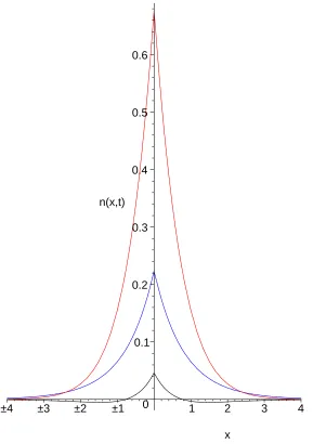
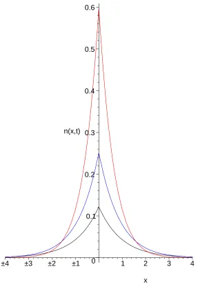
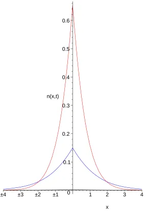
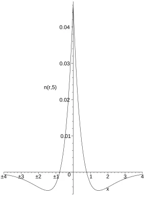
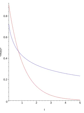
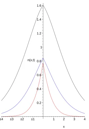
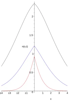
In Figs. 1-3 the infinite domain solution of the equations of Models I, II, and III (Eqs. (88) and (89)) are shown at various times in the case α = 1/2, K = −1, and D = 1. Note that in the case of Model I the solution has become negative and hence is physically unrealistic at t ≈ 5 (Figs. 1 and 4). The reason for this is simply that the reaction term in this model is attempting to remove more walkers than there are available to jump. The solution (Figs. 2 and 3) in the case of the other two models is always positive because we only ever attempt to remove a fraction of the walkers that are available. The solution in the case of Model III decays to zero more rapidly than in the case of Model II.
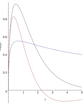
In Figs. 5 and 6, the zeroth order and second order moments are given for each model which are
x(0)(t) =
eKt, Models I, III
Eα,1(Ktα), Model II
(98)
and
x(2)(t) =
2DtαE
1,α(Kt) Model I 2DtαE
α,1(Ktα), Model II
2Dtα Γ (1 +α)e
Kt, Model III
(99)
0 0.1 0.2 0.3 0.4 0.5 0.6
n(x,t)
–4 –3 –2 –1 1 2 3 4
x
FIG. 1: (Color online) The infinite solution for Model I at the dimensionless times t=0.1 (red),
1.0 (blue), and 5.0 (black) with K =−1, D = 1, and α = 1/2. The peak height decreases with
increasing time.
[image:22.595.165.454.69.479.2]0 0.1 0.2 0.3 0.4 0.5 0.6
n(x,t)
–4 –3 –2 –1 1 2 3 4
x
FIG. 2: (Color online) The infinite solution for Model II at the dimensionless times t=0.1 (red),
1.0 (blue), and 5.0 (black) with K =−1, D = 1, and α = 1/2. The peak height decreases with
increasing time.
VI. SUMMARY AND DISCUSSION
[image:23.595.164.454.67.486.2]0 0.1 0.2 0.3 0.4 0.5 0.6
n(x,t)
–4 –3 –2 –1 1 2 3 4
x
FIG. 3: (Color online) The infinite solution for Model III at the dimensionless times t=0.1 (red),
1.0 (blue), and 5.0 (black) with K =−1, D = 1, and α = 1/2. The peak height decreases with
increasing time. The profile att= 5.0 lies along thex axis.
[image:24.595.165.453.69.483.2]0 0.01 0.02 0.03 0.04
n(r,5)
–4 –3 –2 –1 1 2 3 4
x
FIG. 4: (Color online) The infinite solution for Model I at the dimensionless time t=5.0 with
K =−1,D= 1, andα= 1/2.
sub-diffusion with reactions the removal of walkers cannot be performed independent of the diffusion process.
[image:25.595.164.450.69.459.2]0 0.2 0.4 0.6 0.8
<n0(t)>
1 2 3 4 5
t
FIG. 5: (Color online) The zeroth order moments of the infinite solution for Models I and III (red),
and Model II (blue) withK=−1,D= 1, and α= 1/2. The result for Model II is the upper curve
at t= 5.
In Model III the available walkers are added or removed at a constant rate during the time interval between steps. A similar CTRW model was formulated recently for monomolecular reactions [25]. The resultant fractional reaction-diffusion equation that we derived from the CTRW model in this case has a linear reaction dynamics term added to a non standard fractional diffusion term, explicitly, e±ktD(α)
D1−α
e∓kt∂2n
∂x2
. This model equation does not lead to unphysical negative solutions and it recovers the mean field reaction kinetics equation for homogeneous concentrations.
[image:26.595.165.457.62.454.2]0 0.2 0.4 0.6 0.8
<n2(t)>
1 2 3 4 5
t
FIG. 6: (Color online) The second order moments of the infinite solution for Models I (red), II
(blue), and III (black) with K =−1,D = 1, and α= 1/2. Att= 5 the result for Model II is the
upper curve and the result for Model I is the lower curve.
[image:27.595.167.447.65.421.2]0.2 0.4 0.6 0.8 1 1.2 1.4 1.6
n(x,t)
–4 –3 –2 –1 1 2 3 4
x
FIG. 7: (Color online) The infinite solution for Model I at the dimensionless times t=0.1 (red),
1.0 (blue), and 5.0 (black) with K = 1, D = 1, and α = 1/2. The peak height increases with
increasing time.
Acknowledgments
[image:28.595.167.457.62.481.2]0 0.5 1 1.5
2
n(x,t)
–4 –3 –2 –1 1 2 3 4
x
FIG. 8: (Color online) The infinite solution for Model II at the dimensionless times t=0.1 (red),
1.0 (blue), and 2.0 (black) with K = 1, D = 1, and α = 1/2. The peak height increases with
increasing time.
APPENDIX A: RIEMANN-LIOUVILLE FRACTIONAL OPERATORS
The Riemann-Liouville fractional integral is given by ∂−α
∂t−αy(x, t) = 1 Γ(α)
Z t
0
y(x, t)
(t−s)1−αds, α >0. (A1) and the Riemann-Liouville fractional derivative is given by
∂1−α
∂t1−αy(x, t) =
∂ ∂t
1 Γ(α)
Z t
0
y(x, t)
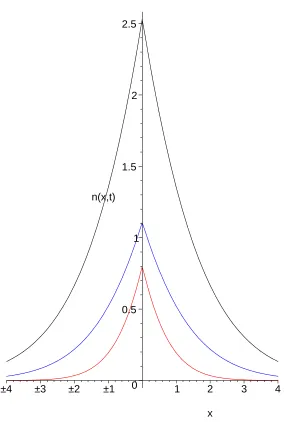
[image:29.595.166.454.65.482.2]0 0.5 1 1.5
2 2.5
n(x,t)
–4 –3 –2 –1 1 2 3 4
x
FIG. 9: (Color online) The infinite solution for Model III at the dimensionless times t=0.1 (red),
1.0 (blue), and 2.0 (black) with K = 1, D = 1, and α = 1/2. The peak height increases with
increasing time.
for 0< α <1. In the paper we have introduced the related operators for 0< α <1,
D1−α[y(x, t)] = ∂1−α
∂t1−αy(x, t) +L
−1
{∂ −α
∂t−αy(x, t)|t=0}, (A3) and
D−α = ∂
−α
[image:30.595.165.455.60.482.2]APPENDIX B: SOLUTION OF LINEAR FRACTIONAL REACTION DIFFU-SION EQUATIONS
In this appendix we consider the infinite domain (Green’s solution) for the general linear fractional reaction-diffusion equation given by
∂n
∂t =D(α)D
1−α∂2n
∂x2 +KD
1−βn (B1)
where the fractional order temporal differential operator D1−α is defined in the paper in Eq.(45).
To solve Models I and II we use an approach similar to that recently described by Lang-lands for modified fractional diffusion equations [41]. First we take the Fourier-Laplace Transform of Eq. (88)
ubbn−bn(q,0) =−D(α)q2u1−αnbb+Ku1−βnbb (B2)
which upon solving for bbn gives
bb
n(q, u) = u
α−1bn(q,0)
uα+Dq2−Kuα−β. (B3)
This can be rewritten in the form (taking into account the initial condition)
bb
n(q, u) = ∞
X
j=0
Kj
j!
j!uα−(1+(β−α)j)
(uα+Dq2)j+1. (B4)
Now from Podlubny [42] we have the Laplace transform of involving the derivative of the Mittag-Leffler function is
Lntαj+β−1E(j)
α,β(−at
α)o(u) = j!uα−β
(uα+a)j+1 (B5)
where the derivative of the Mittag-Leffler function is given by
Eα,β(j)(y) = d jE
α,β(y)
dyj =
∞
X
n=0
(j+n)!yn
n! Γ (α(j+n) +β). (B6)
Setting a=q2, andβ = 1 + (β−α)j in Eq. (B5) we can then invert the Laplace transform
in Eq. (B4) to give
b
n(q, t) = ∞
X
j=0
Ktβj
j! E
(j)
α,1+(β−α)j −q
To invert the Fourier transform we note that the derivative of the Mittag-Leffler function in Eq. (B6) can be written as a Fox function (see e.g., [3])
Eα,β(j)(y) =H11,,21
−y
(−j,1)
(0,1) (1−(αj+β), α)
. (B8)
So to invert the transform in Eq. (B7) we need only to invert, for each j, the term
b
hj(q, t) =E( j)
α,1+(β−α)j −Dq
2tα=H1,1 1,2
Dq2tα
(−j,1)
(0,1) (−βj, α)
. (B9)
To invert the Fourier transform we use the following relation between the Mellin transform of a Fourier transformed function and its Mellin transform in the case of an even function f(x)
M {F [f(x)] (q)}(z) = 2 Γ (z) cosπz 2
M {f(x)}(1−z). (B10)
So to invert the Fourier transform, bhj(q, t), in Eq. (B9) we need to first evaluate its Mellin transform to find the Mellin transform of hj(x, t) using Eq. (B10). The Mellin transform then need only be inverted to find the Fourier inverse, hj(x, t).
Taking the Mellin transform of Eq. (B9) using the Mellin transform of a Fox function [43], the identity [44]
M {φ(axp)
}(z) = 1 pa
−zp
M {φ(x)}
z p
p >0, a >0 (B11)
and Eq. (B10) we find
M {hj(x, t)}(z) = 1 2
1 √
4πDtα
1 √
4Dtα
−z
Γ z
2
Γ 1 2 +j+
z
2
Γ 1− α
2 +βj+
αz
2
. (B12)
Inverting the Mellin transform Eq. (B12) and noting x=|x| we find
hj(x, t) = 1 2
1 √
4πDtαH
2,0 1,2
√|x|
4Dtα
1− α
2 +βj,
α
2
0,1 2
1
2 +j, 1 2
. (B13)
Using the identity
Hm,n p,q x
(ap, αp) (bq, βq)
=cHm,n
p,q
xc
(ap, cαp) (bq, cβq)
(B14)
with c= 12 we arrive at the expression forhj(x, t):
hj(x, t) = 1 √
4πDtαH
2,0 1,2
x2
4Dtα
1− α2 +βj, α
(0,1) 12 +j,1
The infinite domain (Green’s solution) of Eq. (88) by Eqs (B7) and (B15),
n(x, t) = √ 1 4πDtα
∞
X
j=0
Ktβj
j! H
2,0 1,2
x2
4Dtα
1− α
2 +βj, α
(0,1) 12 +j,1
. (B16)
[1] D. ben Avraham S. Havlin,Diffusion and Reactions in Fractals and Disordered Systems
(Cam-bridge University Press, Cam(Cam-bridge, UK, 2000).
[2] J.-P. Bouchard and A. Georges, Phys. Rep. 195, 127 (1990). [3] R. Metzler and J. Klafter, Phys. Rep. 339, 1 (2000).
[4] R. Metzler and J. Klafter, J. Phys. A. 37, R161 (2004). [5] G. Drazer and D.H. Zanette, Phys. Rev. E60, 5858 (1999). [6] E. Weeks and D. Weitz, Chem. Phys.284, 361 (2002).
[7] M. Weiss, H. Hashimoto, and T. Nilsson, Biophys. J. 84, 4043 (2003).
[8] K. Ritchie, X.-Y. Shan, J. Kondo, K. Iwasawa, T. Fujiwara, and A. Kusumi, Biophys. J. 88, 2266 (2005).
[9] M.J. Saxton, Biophys. J.81, 2226 (2001).
[10] I.M. Sokolov and J. Klafter, Chaos15, 026103 (2005). [11] B.I. Henry and S.L. Wearne, Physica A 276, 448 (2000).
[12] B.I. Henry and S.L. Wearne, SIAM Journal of Applied Mathematics 62, 870 (2002). [13] M.O. Vlad and J. Ross, Physical Review E 66, 061908 (2002).
[14] S. Fedotov and V. Mendez, Physical Review E66, 030102(R) (2002).
[15] J. Sung, E. Barkai, R.J. Silbey, and S. Lee, J. Chem. Phys. 116, 2338 (2002). [16] K. Seki, M. Wojcik, and M. Tachiya, Journal of Chemical Physics 119, 2165 (2003). [17] K. Seki, M. Wojcik, and M. Tachiya, Journal of Chemical Physics 119, 7525 (2003). [18] M. Fukunaga, Int. J. Appl. Math 14, 269 (2003).
[19] S.B. Yuste, L. Acedo, and K. Lindenberg, Phys. Rev. E 69, 036126 (2004). [20] V. Mendez, D. Campos, and S. Fedotov, Phys. Rev. E. 70, 036121 (2004). [21] V. Mendez and V. Ortega-Cejas, Phys. Rev. E71, 057105 (2005).
[22] B.I. Henry, T.A.M. Langlands, and S.L. Wearne, Phys. Rev. E72, 026101 (2005).
[23] B.I. Henry, T.A.M. Langlands, and S.L. Wearne, in Proceedings of the First International
Machado, J. Trigeassou, and J. Sabatier (International Federation of Automatic Control,
Bordeaux, France, 2004), pp. 113–120.
[24] T.A.M. Langlands, B.I. Henry, and S.L. Wearne, J. Phys. C (2006, submitted).
[25] I.M. Sokolov, M.G.W. Schmidt, and F. Sagues, Phys. Rev. E73, 031102 (2006). [26] G. Hornung, B. Berkowitz, and N. Barkai, Phys. Rev. E72, 041916 (2005). [27] E. Montroll and G. Weiss, J. Math. Phys.6, 167 (1965).
[28] H. Scher and M. Lax, Phys. Rev. B. 7, 4491 (1973). [29] K. Pearson, Nature72, 294 (1905).
[30] J. Klafter, A. Blumen, and M.F. Shlesinger, Phys. Rev. A 35, 3081 (1987). [31] F. Mainardi, M. Raberto, R. Gorenflo, and E. Scalas, Physica A287, 468 (2000).
[32] J.D. Murray, Mathematical Biology. I: An Introduction (Springer-Verlag, New York, 2003),
3rd ed.
[33] A. Compte and R. Metzler, J. Phys. A 30, 7277 (1997).
[34] B. Beamer, D.A. Benson, and M.M. Meerschaert, Physica A350, 245 (2004). [35] P. Paradisi, R. Cesari, F. Mainardi, and F. Tampieri, Physica A 293, 130 (2001).
[36] W. Feller, An Introduction to Probability Theory and its Applications. Vol II (Wiley, New
York, 1966), 2nd ed.
[37] G. Margolin and B. Berkowitz, Physica A.334, 46 (2004).
[38] E. Scalas, R. Gorenflo, and F. Mainardi, Phys. Rev. E 69, 011107 (2004).
[39] G. Hornung, B. Berkowitz, and N. Barkai, Electronic Physics Auxiliary Publication pp. no.
E–PLEEE8–72–051510 (2005).
[40] K. Miller and B. Ross,An Introduction to the Fractional Calculus and Fractional Differential
Equations (John Wiley & Sons, New York, 1993).
[41] T.A.M. Langlands, Physica A367, 136 (2006).
[42] I. Podlubny, Fractional Differential Equations, vol. 198 ofMathematics in Science and
Engi-neering (Academic Press, New York and London, 1999).
[43] H. Srivastava, K. Gupta, and S. Goyal, The H-Functions of One and Two Variables with
Applications (South Asian Publishers Pvt Ltd, New Delhi, 1982).