Combination of Lidar and Model Data for Studying Deep Gravity Wave Propagation

Combination of Lidar and Model Data for Studying Deep Gravity Wave

Propagation

BENEDIKTEHARD*ANDPEGGYACHTERT1

Department of Meteorology, Stockholm University, Stockholm, Sweden

ANDREASDÖRNBRACK ANDSONJAGISINGER

Deutsches Zentrum fur Luft- und Raumfahrt, Institut f€ ur Physik der Atmosph€ €are, Oberpfaffenhofen, Germany

JÖRGGUMBEL ANDMIKHAILKHAPLANOV

Department of Meteorology, Stockholm University, Stockholm, Sweden

MARKUSRAPP#

Deutsches Zentrum fur Luft- und Raumfahrt, Institut f€ ur Physik der Atmosph€ €are, Oberpfaffenhofen, Germany

JOHANNESWAGNER*

Institute of Meteorology and Geophysics, University of Innsbruck, Innsbruck, Austria

(Manuscript received 8 December 2014, in final form 5 August 2015)

ABSTRACT

The paper presents a feasible method to complement ground-based middle atmospheric Rayleigh lidar temperature observations with numerical simulations in the lower stratosphere and troposphere to study gravity waves. Validated mesoscale numerical simulations are utilized to complement the temperature below 30-km altitude. For this purpose, high-temporal-resolution output of the numerical results was interpolated on the position of the lidar in the lee of the Scandinavian mountain range. Two wintertime cases of oro-graphically induced gravity waves are analyzed. Wave parameters are derived using a wavelet analysis of the combined dataset throughout the entire altitude range from the troposphere to the mesosphere. Although similar in the tropospheric forcings, both cases differ in vertical propagation. The combined dataset reveals stratospheric wave breaking for one case, whereas the mountain waves in the other case could propagate up to about 40-km altitude. The lidar observations reveal an interaction of the vertically propagating gravity waves with the stratopause, leading to a stratopause descent in both cases.

* Current affiliation: Deutsches Zentrum für Luft- und Raumfahrt, Institut für Physik der Atmosphäre, Oberpfaffenhofen, Germany. 1_{Current affiliation: Institute of Climate and Atmospheric Science, School of Earth and Environment, University of Leeds, Leeds,}

United Kingdom.

#_{Additional affiliation: Meteorological Institute Munich, Ludwig-Maximilians-Universität München, Munich, Germany.}

Corresponding author address: Benedikt Ehard, Deutsches Zentrum für Luft und Raumfahrt, Institut für Physik der Atmosphäre, Münchener Str. 20, 82234 Oberpfaffenhofen, Germany.

E-mail: benedikt.ehard@dlr.de Denotes Open Access content.

DOI: 10.1175/MWR-D-14-00405.1

1. Introduction

During the last decades, internal gravity waves have been studied intensely because of their importance for the circulation and structure of the middle atmosphere (Fritts and Alexander 2003). The most energetic part of the gravity wave spectrum is excited in the troposphere, with prominent source mechanisms being the flow over topography (e.g., Smith et al. 2008), convection (e.g., Vadas et al. 2012), flow deformation, and vertical shear at upper-level fronts (Plougonven and Zhang 2014). As in-ternal gravity waves distribute energy and momentum in the atmosphere, they represent a prominent coupling mechanism between the troposphere and the middle at-mosphere (e.g.,Fritts and Alexander 2003).

The amount of gravity wave activity arriving in the middle atmosphere is considerably affected by the back-ground flow in the troposphere and stratosphere. Dissi-pation or reflection can hinder the propagation of gravity waves into the mesosphere (i.e., the deep wave propaga-tion). Vertical levels where the component of the back-ground wind in the direction of wave propagation equals the horizontal phase speed are called critical levels. There, either total or partial critical level filtering (seeTeixeira 2014) impedes the vertical propagation of gravity waves (e.g.,Whiteway and Duck 1996). Often, the waves break and deposit their momentum at these levels (e.g., Dörnbrack 1998). The dissipation leads to deviations from the radiative equilibrium flow state at higher altitudes (e.g., Siskind 2014). Thereby, the wind field and the thermal structure of the middle atmosphere are modified (e.g.,Lindzen 1981;Holton and Alexander 2000).

Internal gravity waves have been measured and ana-lyzed with a large variety of active and passive remote sensing techniques as well as with in situ observations. These observational tools include airborne and ground-based lidars (e.g.,Alexander et al. 2011;Dörnbrack et al 2002;Rauthe et al. 2008;Williams et al. 2006), radars (e.g., Stober et al. 2013), airglow imagers (e.g.,Suzuki et al. 2010), noctilucent cloud images (e.g.,Pautet et al. 2011), satellite measurements (e.g.,Alexander et al. 2008), radiosonde soundings (e.g.,Dörnbrack et al. 1999;Zhang and Yi 2005), and rocket soundings (e.g., Rapp et al. 2004). However, these instruments are limited to par-ticular altitude ranges and are only sensitive to a dis-tinct part of the gravity wave spectrum (Gardner and Taylor 1998;Preusse et al. 2009). Therefore, various instruments and measurement techniques must be com-bined to cover the different altitude ranges and to obtain a comprehensive picture of the gravity wave spectrum (e.g.,Bossert et al. 2014;Goldberg et al. 2004;Takahashi et al. 2014). Furthermore, complementary linear theory or numerical modeling is a necessary prerequisite to

understand the characteristics and propagation properties of the observed gravity waves.

The approach of the Role of the Middle Atmosphere in Climate (ROMIC)1project ‘‘Investigation of the life cycle of gravity waves’’ (GW–LCYCLE) is to combine ground-based, airborne, and spaceborne instruments to measure the excitation, propagation, and dissipation of vertically propagating gravity waves on their way into the middle atmosphere.

A first field campaign (GW–LCYCLE I) was con-ducted in northern Scandinavia from 2 to 14 December 2013. GW–LCYCLE I studied the deep propagation of mountain waves excited by the flow across the Scandi-navian Alps by a variety of ground-based and airborne instruments. The instrumentation comprised airglow imagers, lidars, and radars at Alomar and Esrange; co-ordinated balloon soundings from Andøya (698N, 168E), Esrange (688N, 218E), Kiruna (688N, 208E), and Sodankylä (678N, 278E) (Fig. 1); and in situ and remote sensing in-struments onboard the research aircraft Falcon, operated by the German Aerospace Center (DLR). Of all the in-struments participating in GW–LCYCLE I, the ground-based lidars were so far the only ones that provided the temporal and spatial resolution necessary for resolving low- and medium-frequency gravity waves over the entire altitude range from the lower stratosphere up to the middle atmosphere (Fritts and Alexander 2003;Rauthe et al. 2008). The disturbing presence of aerosols below about 30-km altitude allows a retrieval of temperature or

FIG. 1. Map of the outer domain as used for the mesoscale sim-ulations conducted with the WRF Model. The inner domain is shown by the black square. The red dots represent the observation sites And_øya (A), Kiruna (K), Esrange (E), and Sodankyl_ä(S).

1_{ROMIC is a research initiative funded by the German ministry}

density perturbations from Rayleigh lidar measurements exclusively above this altitude. Therefore, the deep gravity wave propagation from the troposphere into the middle atmosphere could not be studied with these lidars alone.

In this paper, Rayleigh lidar temperatures measured by the Esrange lidar on 3–4 and 13–14 December 2013 are used between 30- and 65-km altitude. Below this altitude range, the lidar observations are complemented with temperatures simulated numerically by the Advanced Research version of the Weather Research and Fore-casting (WRF) Model (ARW; Skamarock and Klemp 2008). Our goal is to determine the wave characteristics from the lower troposphere to the mesosphere. For this purpose, we combine and analyze the lidar tem-perature measurements and the validated mesoscale simulation results.

Prerequisites of this approach are high-resolution numerical simulations in space and time of the tropo-spheric and stratotropo-spheric flow above Scandinavia. Ideally, one would utilize mesoscale simulations up to the maximum altitude of the lidar observations at 65 km. However, most of the recent mesoscale stratospheric simulations extend only up to approximately 40 km or even lower. Additionally sponge layers are necessary to attenuate gravity waves below the model top (e.g., Dörnbrack et al. 2001; Limpasuvan et al. 2007,2011; Plougonven et al. 2015).

Global meteorological analysis and forecast fields constitute an alternative to mesoscale simulations. For example,Khaykin et al. (2015) combined global-scale temperature analysis with Rayleigh lidar temperature measurements to generate a 7-yr climatology of gravity wave activity. In their study, nighttime means are used to calculate weekly and monthly means. For our study, the European Centre for Medium-Range Weather Forecasts (ECMWF) Integrated Forecast System (IFS) could provide hourly vertical temperature profiles above Esrange up to 80-km altitude. However, artificial numer-ical horizontal diffusion2 dampens higher-frequency modes starting already at about 30-km altitude. Be-sides this damping, the 1-h temporal resolution is con-sidered to be insufficient for combination with the 15-min lidar profiles. Therefore, we decided to conduct mesoscale simulations that provide a high spatial (2000 m) and temporal (300 s) resolution up to about 41-km altitude with a 10-km-thick sponge layer. Since there is a lack of an overlapping region between the WRF and the lidar data, no direct intercomparison is pos-sible. Instead, radiosonde and aircraft temperature

data are used to assure that the gravity wave structures contained in the model are realistic.

The feasibility of our approach is demonstrated for two selected cases from GW–LCYCLE I. These cases were observed by the DLR research aircraft Falcon, by extensive radiosoundings, and by lidar measurements on 3–4 December and 13–14 December 2013. The respec-tive periods are characterized by strong-to-moderate tropospheric forcing, which excited mountain waves over northern Scandinavia. Forcing conditions are con-sidered to be moderate if the component of the wind at 700 hPa perpendicular to the Scandinavian mountain ridge is smaller than 15 m s21, whereas strong forcing occurs if the wind component is larger than 15 m s21. Ambient westerly winds in the stratosphere favored the propagation of mountain waves in both cases.

The gravity wave analysis of the combined dataset derives vertical wavelength and gravity wave potential energy density using the observed and simulated tem-perature deviations from the estimated background profiles. Additionally, the WRF Model output provides quantities like wind, vertical energy fluxes, and stability parameters (Richardson number and displacement of isentropic surfaces) in the troposphere and lower stratosphere. Thus, results of the combined dataset enable a more comprehensive characterization of grav-ity wave excitation and propagation. Our results should encourage other scientists to apply this kind of an ap-proach to past and future datasets of middle atmo-spheric lidar measurements.

Section 2provides an overview of the methodological approach of this study, starting with a description of the instruments and tools used. The results are presented in section 3and discussed in detail insection 4. Finally, the conclusions are given insection 5.

2. Methodology

a. Ground-based lidar measurements

The Department of Meteorology of Stockholm Uni-versity operates the Esrange lidar at Esrange (688N, 218E) near the Swedish city of Kiruna. The Esrange lidar uses a frequency doubled neodymium-doped yttrium aluminum garnet (Nd:YAG) solid-state laser as a light source with a pulse repetition rate of 20 Hz and a pulse energy of 900 mJ. A detection range gate of 1ms results in a vertical resolution of 150 m. The parallel polarized Rayleigh signal covers the altitude range between 4 and 80 km. Further technical details of the system can be found in Blum and Fricke (2005) and Achtert et al. (2013). Assuming hydrostatic equilibrium, the measured density profile is integrated downward in order to obtain

an atmospheric temperature profile, as first proposed by Hauchecorne and Chanin (1980). The initialization al-titude of the integration technique was chosen to be the altitude where the count rate is four counts higher than the background count rate. The determination of the temperature profiles is limited to an altitude range between 30 and 65 km. The upper boundary of the temperature measurements suitable for gravity wave analysis was chosen in order to ensure a balance be-tween accuracy and altitude range. The lower boundary arises because of the presence of aerosols in the lower stratosphere, which limits the application of the in-tegration technique. For further details concerning measurement uncertainties, seeEhard et al. (2014).

The measured Rayleigh signal is integrated over 5000 laser pulses (approximately 4.2 min) for noise reduction purposes. Vertical temperature profiles are determined as sliding 1-h averages of the Rayleigh lidar measure-ments every 15 min. To further reduce the noise, these profiles are smoothed vertically with a running mean of a window length of 2 km. The resulting temperature profiles are binned to 2-km-wide altitude intervals, and a sliding cubic spline is used to determine the background temperature (e.g., Duck et al. 2001; Alexander et al. 2011). The background temperature profiles are then subtracted from the temperature profiles to obtain the temperature perturbations.

b. Airborne observations

The in situ temperature measurements onboard the DLR research aircraft Falcon in a temporal resolution of 1 Hz and with an accuracy of 0.5 K are used to verify the mesoscale numerical simulations. Only horizontal flight legs on 3 and 13 December 2013 are analyzed, which results in a total of more than 7 h of measurements (Table 1). Additionally, the temperature measurements are used to estimate the horizontal wavelengths along extended west–east transects across the Scandinavian mountain ridge during the two events.

c. Radiosonde observations

During GW–LCYCLE I balloonborne measurements of temperature, relative humidity, pressure, and wind were conducted at Andøya, Kiruna Airport, Esrange, and Sodankylä, respectively. In this study, the 21 ra-diosondes (Vaisala RS-92) released from Esrange are used to validate the WRF numerical simulations in the lowest 30 km of the atmosphere. The RS-92 has a ca-pacitive temperature sensor with a total accuracy better than 0.5 K and GPS-wind measurement with 0.15 m s21 and 28accuracy in wind speed and wind direction, re-spectively (Vaisala 2014). The mean balloon ascent rate of 5 m s21leads to a vertical resolution of about 10 m.

Because of the large horizontal winds during the mountain wave events, the balloonborne measurements were taken along strongly tilted trajectories. Therefore, the sounding profiles cannot provide pure vertical pro-files like the lidar observations, since they contain a combination of vertical and horizontal information of the atmospheric state. The radiosondes analyzed in this study drifted horizontally up to 270 km, depending on wind conditions.

d. Global meteorological data

Operational analyses of the ECMWF IFS are used to provide meteorological data to characterize the atmo-spheric situation and to serve as initial and boundary data for the mesoscale numerical simulations. The analysis fields of the IFS cycle 40r1 have a horizontal resolution of about 16 km (T1279) and 137 vertical model levels (L137). The model top of the T1279/L137 IFS was located at 0.01 hPa.

e. Mesoscale numerical simulations

To derive gravity wave parameters in the troposphere and the lower stratosphere, mesoscale simulations were performed with the WRF Model, version 3.4 (Skamarock et al. 2008). The numerical model used two nested do-mains over northern Scandinavia with horizontal grid resolutions of 6 and 2 km, respectively (Fig. 1). The inner domain is computed by one-way nesting. In the vertical, 131 terrain-following levels are applied, with level dis-tances reaching from 50 m near the surface to 160 m at about 1.6-km height. In the troposphere (between 1.6- and 10-km height), the level distances are kept

TABLE1. Horizontal flight legs of the DLR Falcon aircraft on 3 and 13 Dec 2013. The legs were generally oriented parallel to the horizontal wind speed and, thus, almost perpendicular to the Scandinavian mountain ridge.

Flight leg Length (km) Altitude (km)

131203_1 184.7 5.6

131203_2 601.8 7.3

131203_3 228.5 5.5

131203_4 472.1 7.2

131203_5 433.5 9.2

131203_6 323.1 10.4

131213_1 239.9 5.7

131213_2 484.3 5.7

131213_3 475.6 7.4

131213_4 246.8 10.1

131213_5 112.5 11.3

131213_6 67.3 11.3

131213_7 317.6 5.7

131213_8 111.4 10.8

131213_9 433.4 7.5

nearly constant between 160 and 180 m. Above 10-km height, the level distances are stretched to level dis-tances of about 600 m at the model top, which is located at 1 hPa, corresponding to about 41 km. To avoid wave reflections at the model top, a Rayleigh damping layer was added at the uppermost 10 km (Klemp et al. 2008). Different model tops and sponge layer depths were tested while conducting this study. Simulations with a model top higher than 1 hPa were found to become unstable. Currently, we do not know why this is the case but will investigate this issue in the future. The initial and boundary conditions for the WRF Model are sup-plied by ECMWF operational analysis on 137 model levels with a temporal resolution of 6 h. Further details about the model setup can be found in theappendix.

The complete WRF output is available every 60 and 30 min for the outer and inner domain, respectively. In addition, the momentary basic fields like wind, pressure, temperature, water vapor mixing ratio, and the Brunt– Väisäläfrequency are stored every 5 min for the inner domain to obtain a temporal resolution similar to the lidar raw data. This high-resolution output enables the combination and comparison of WRF simulations with lidar, aircraft, and radiosonde data.

The numerical WRF Model is commonly used for many different atmospheric phenomena [e.g., polar lows (Wagner et al. 2011), tropical cyclones (Davis et al. 2008), downslope winds (Steinhoff et al. 2013), and nonorographic gravity waves (Plougonven et al. 2015)], and its performance has been validated thoroughly (e.g., Wagner et al. 2011;Hu et al. 2010;Wu and Petty 2010). However, the application to the flow over steep topog-raphy and to the excitation, propagation, and breaking of mountain waves are outstanding challenges, and the success often depends on the appropriate choice of vertical levels, physical parameterizations, domain lo-cations, etc. (e.g.,Doyle et al. 2011).

The accuracy of the WRF simulations is examined by comparing 21 high-vertical-resolution radiosondes launched at Esrange during December 2013 against the WRF simulations. For this purpose, the numerical re-sults are interpolated in time and space to the individual radiosonde trajectories. Another comparison is realized using the flight level in situ data measured by the DLR research aircraft Falcon and the WRF results interpo-lated in space and time along the respective flight legs (Table 1). Both Falcon in situ data and WRF flight level data were averaged over 5 s, resulting in a horizontal resolution of approximately 1 km.

f. Combination of lidar and model data

The high-resolution 5-min WRF data were used to complement the lidar data in the troposphere and lower

stratosphere up to an altitude of 30 km. For this purpose, the three-dimensional temperature fields of the nu-merical model were interpolated on a one-dimensional vertical beam at the location of the Esrange lidar for every output time. The horizontally interpolated verti-cal temperature profiles were then interpolated to the same vertical grid as specified by the Esrange lidar ob-servations and averaged over the same time spans. The WRF vertical temperature profiles are relatively smooth compared to the lidar data because of the numerical scheme minimizing spurious oscillations at grid scale. Thus, no additional smoothing was applied.

Finally, temperature perturbations were determined applying the same method for the combined dataset as described for the lidar data insection 2a. In this way, the combined dataset from lidar and WRF data possesses the same temporal and spatial resolutions. The combi-nation of both datasets enables us to analyze wave pa-rameters and to study the vertical propagation of mountain waves from the troposphere to the middle atmosphere.

g. Analysis method

The gravity wave activity is described by the gravity wave potential energy density (GWPED) per volume calculated from

E_p,vol5r₀1 2 g2 N2 T0 T₀ 2 and (1)

with N25 g T₀ dT₀ dz 1 g c_p ! , (2)

Spectral properties of gravity waves are determined by means of a wavelet transformation (e.g., Torrence and Compo 1998). Wavelet spectra of individual tem-perature perturbation profiles are calculated using the Morlet wavelet of sixth order. To reduce errors at the edges of the finite data series, the end of the data series is padded with zeros before applying the wavelet trans-formation, which assumes the data is cyclic, and calcu-lating the wavelet coefficients. The cone of influence (COI) is the region of the wavelet spectrum where edge effects become important. Outside the COI, the spectral amplitude could be reduced because of the zero padding (Torrence and Compo 1998). The absolute values of the individual spectra are averaged over a given time period to retrieve the mean spectrum for an observational pe-riod. Dominant vertical wavelengths are derived by examining the local maxima in the global mean wavelet spectrum, defined as the wavelet spectrum averaged with altitude (Torrence and Compo 1998).

The vertical fluxes of wave energy,

E_flux,vert5hp0w0i, (3)

with pressure perturbationp0and vertical velocity per-turbationw0, are computed from the WRF simulations according toKruse and Smith (2015): After interpolat-ing the pressure and velocity fields to the desired height levels, a high-pass filter with a filter length of 300 km is applied in Fourier space, which yields the small-scale perturbations p0 and w0. The energy flux field is then obtained by the pointwise multiplication of these per-turbations [Eq.(3)] and applying a low-pass filter with a filter length of 150 km, resulting in a smoothing of the energy flux. The brackets in Eq. (3) denote an aver-aging over the region 668–708N and 108–258E, including the upstream and downstream regions of the northern Scandinavian mountain ridge.

3. Results

a. Meteorological conditions in November and December 2013

In November and December 2013 the westerly flow across the mountains was often aligned with the evolving polar night jet. This flow constellation is known to excite mountain waves and to facilitate their vertical propa-gation into the lower and middle stratosphere (e.g., Dörnbrack et al. 2001).

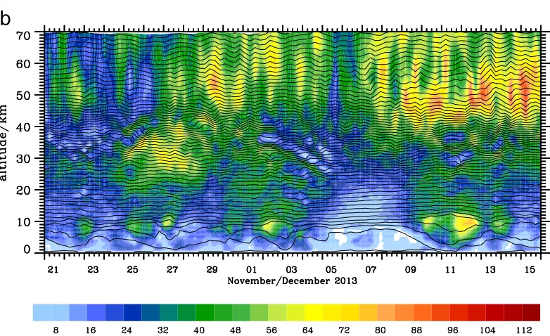
Figure 2presents the temporal evolution of temper-ature and wind above Esrange for the period from 21 November to 15 December 2013. The atmospheric parameters are taken from 6-hourly operational ana-lyses of the IFS. The vertical temperature distribution

shows a cold stratosphere with minimum temperatures of less than 190 K at about 30-km altitude and a warm stratopause above (Fig. 2a). The overall evolution re-veals variations in the absolute values as well as in the altitude of the respective temperature layers indicative of the early formation phase of the polar vortex. Addi-tionally, the stratospheric temperature and potential temperature are often disturbed by wavelike perturba-tions (e.g., around 24–25 November, 27–28 November, 3–4 December, and 11–13 December), which turn out to be periods when mountain waves were excited by the flow across the Scandinavian mountain ridge. These pertur-bations are correlated with an enhanced tropospheric wind and a jet stream near the tropopause (Fig. 2b). Most noticeable are the downward-propagating wind anoma-lies in the period 3–4 December 2013. The upper-stratospheric and mesospheric winds show a remarkable variability, which probably results from planetary waves disturbing the polar vortex during this period.

We selected two cases of enhanced observed wave activity to analyze the wave properties and to demon-strate the feasibility of the data combination. The first period on 3–4 December 2013 represents a case of strong westerly flow of about 30 m s21at 700 hPa (Fig. 3a) and a tropopause jet at 300 hPa with about 40 m s21(Fig. 3b). The meteorological situation on 3–4 December 2013 is characterized by a slowly northeastward propagating trough. This cyclonic flow led to a strong cross-mountain component of the wind. In the lower stratosphere be-tween 30 and 10 hPa (Figs. 3c and 2b), the wind was nearly uniform with about 30 m s21but increased slightly above to values of about 60 m s21 at 1 hPa (Fig. 3d). Those tropospheric and lower-stratospheric winds favor the excitation and vertical propagation of mountain waves. However, the ECMWF analyses only indicate wave patterns up to an altitude of about 30 km (Figs. 2b and3b–d), which is approximately the altitude were the model damping by horizontal diffusion starts. Thus, it remains open if the waves could propagate into the mesosphere.

mountain waves were excited and the stronger strato-spheric winds at the inner edge of the polar vortex fa-vored their vertical propagation (Figs. 4c,d).

b. Validation of the WRF Model simulations

The validation of the high-resolution numerical sim-ulations was conducted for a total of 21 radiosonde

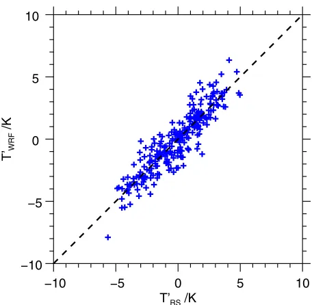
launches. For the comparison, WRF results were inter-polated to the trajectories of the individual radiosondes. Temperature perturbations were calculated for 2-km-wide altitude bins by means of the sliding spline method mentioned above insection 2a. The comparison of WRF and radiosonde temperature perturbations is shown in Fig. 5for data up to 30-km altitude. This reveals that

FIG. 2. Time–height sections of the (a) absolute temperature (K; color coded) and the (b) horizontal wind (m s21_;

temperature perturbations determined from the WRF simulations and radiosoundings are well correlated. The linear Pearson correlation coefficient of WRF and ra-diosonde temperature perturbations is 0.912. Compar-ing the absolute temperatures simulated by the WRF Model and those measured by the radiosondes results in a correlation coefficient of 0.998. The root-mean-square error is defined as

A_RMSE5

ffiffiffiffiffiffiffiffiffiffiffiffiffiffiffiffiffiffiffiffiffiffiffiffiffiffiffiffiffiffiffiffiffiffiffiffiffiffiffiffi

å

i

(A_i,WRF2A_i,RS)2 n

v u u t

, (4)

whereAis eitherT0orT, andnis the total number of values used. The comparison of WRF and radiosonde data yieldsT_RMSE0 50.96 K andTRMSE51.40 K for data up to 30-km altitude. If one considers only values up to

20-km altitude, both values decrease toT_RMSE0 50.76 K andTRMSE50.99 K.

To compare the spectral characteristics of the ob-served and simulated gravity waves, we calculated the wavelet spectrum of the temperature perturbations separately for both datasets. To identify the resolved scales, data with a vertical resolution of 100 m were analyzed.Figures 6a–c show the temperature pertur-bations derived from three radiosonde launches on

3 December 2013 (red lines) and the corresponding WRF simulations (blue lines). Figures 6d–f show the wavelet spectra for these three radiosonde launches, whereas Figs. 6g–i show the corresponding wavelet spectra for the WRF simulations.

Figures 6a–cshow a general agreement of the phase as well as the amplitude between the measured and simu-lated temperature perturbations. Note that the tem-perature perturbations are calculated using a vertical

spacing of 100 m. The agreement between the radio-sonde measurements and the WRF simulations in-creases further if the altitude resolution is reduced to 2 km, which is the altitude resolution used for the com-bination of lidar and model data.

ComparingFigs. 6d–ftoFigs. 6g–i, a strong similarity between the radiosonde and the WRF spectra can be seen. Especially the vertical wavelengths and the cor-responding altitude regions of dominant wave modes agree very well. However, the amplitudes of the domi-nant wave modes differ by about 1–2 K. This difference has the same order of magnitude as the RMSE of the 2-km binned temperature perturbationsT_RMSE0 (Fig. 5). The strong similarity of the vertical wavelet spectra, together with the low values ofT_RMSE0 , indicate that the WRF Model is capable of not only reproducing the vertical wavelength but also the phase of the gravity waves. Furthermore, radiosondes have a larger spectral amplitude and a larger variability than the WRF Model at scales smaller than 4 km (Fig. 6). The representation of small-scale gravity waves by the WRF Model does not affect the analysis of the combined dataset, since the data is averaged over 2 km, as described insection 2a.

Additionally, we compared the Falcon in situ tem-perature measurements and the WRF data interpolated along horizontal flight legs on 3 and 13 December 2013

(seeTable 1for leg details). The RMSE for the com-parison of the 5-s-averaged Falcon in situ and WRF absolute temperature is 0.53 K, which is comparable in magnitude to the measurement accuracy of 0.5 K of the Falcon in situ temperature measurements. The com-parison reveals that the radiosonde and airborne mea-surements are well reproduced by the numerical simulations.

c. Lidar temperature observations

Figure 7provides a time–height section of the tem-peratures determined from the Esrange lidar in the al-titude range of 30–65 km between 24 November and 15 December 2013, thus extending the GW–LCYLCE I campaign. Altogether, there are approximately 130 h of lidar observations suitable for gravity wave analysis. There are several continuous periods of lidar measure-ments showing a perturbed stratopause region. Gener-ally, and in agreement with the ECMWF profiles (Fig. 2a), the stratopause is warmer and exhibits larger altitude variations in December 2013 compared to November 2013.

In the following, the two observational periods of in-terest, as mentioned insection 3a, are described in more detail. Both periods are characterized by a descending stratopause. During 3–4 December 2013, the absolute temperatures measured by the lidar show a cooling of the stratopause (50–60-km altitude range) at the be-ginning of the period until 0000 UTC 4 December. The descending stratopause is followed by a narrower warm downwelling layer above 60-km altitude at around 0200 UTC 4 December 2013 (Fig. 7). The consecutive ECMWF analyses (Fig. 2a) partly reproduce the stra-topause descent but do not simulate the observed tem-perature maximum in the narrow downwelling layer at 65-km altitude. Furthermore, temperatures simulated by ECMWF are slightly lower than the lidar tempera-tures above 50-km altitude.

At the beginning of the last observational period on 13–14 December 2013, the stratopause region is almost isothermal for a period of 6 h. Around 1900 UTC, the stratopause gets warmer at approximately 54-km alti-tude and descends until 0800 UTC 14 December by al-most 10 km. The ECMWF analyses (Fig. 2a) reproduce the isothermal stratopause region, but the descent of the forming stratopause is analyzed at a later time. Also, the stratopause height is lower in the ECMWF analyses compared to the lidar measurements.

d. Wave analysis

In the following, we present the gravity wave analysis of the combined dataset for the two selected cases on 3– 4 December 2013 and 13–14 December 2013.

1) 3–4 DECEMBER2013

As mentioned above, the overall meteorological conditions favored the excitation of mountain waves and their further propagation into the stratosphere. The leeward descent of air led to gaps in the low-level clouds allowing for intermittent lidar observations over a pe-riod of almost 18 h. Figure 8a shows the temperature perturbations obtained by combining the Esrange lidar and the numerical model data on 3–4 December 2013.

The most prominent features ofFig. 8aare the slightly descending bands of positive and negative temperature anomalies throughout the entire altitude range until 0000 UTC 4 December 2013. At 0000 UTC, there is a reduction of amplitudes and a shift in height of

the anomaly bands. Afterward, they remain almost at constant altitudes. After about 0300 UTC, the anom-alies descend again, and the amplitude is increased at altitudes above 30 km. The descending temperature anomalies in time can be interpreted as propagating waves, while the patterns without altitude changes represent standing waves (i.e., stationary mountain waves).

In general, the amplitude of the temperature fluctua-tions grows with altitude. This is mainly caused by the amplification of the gravity waves’ amplitude due to decreasing density. However, other factors, such as the local wind conditions, are potential contributors as well. Moreover, the phase lines above 40 km appear less structured than below this altitude. We hypothesize that

this could be a superposition of internal gravity waves from different sources.

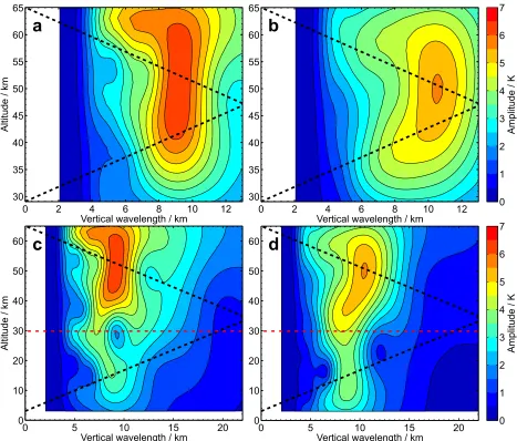
Figure 9ashows the mean wavelet spectrum for the lidar data between 30- and 65-km altitude for this case, whereas Fig. 9cdepicts the corresponding analysis for the combined dataset of the lidar observations and the numerical simulation results. The Rayleigh lidar data above 30 km display a dominant wavelength of lz ’ 9 km. There is a broadening of the spectrum with alti-tude. The combined wavelet spectrum retains the dominant wave mode above 40-km altitude. At lower altitudes, the spectral distribution becomes bimodal, with modes centered aroundlz’7 km andlz’12 km, respectively. Interestingly, the spectral amplitude for lz ’9 km is strongly reduced near 30-km altitude di-rectly below the maximum above.

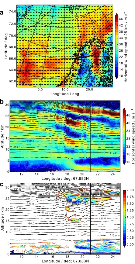
Horizontal and vertical cross sections of the WRF simulation results valid at 0100 UTC 4 December 2013 are presented inFig. 10. The horizontal wind at 25-km

altitude is maximum above the Norwegian coastline and farther downstream between Sweden and Finland. The dominant horizontal wavelength estimated from the difference of consecutive horizontal wind minima amounts tolh’ 400 km.

The vertical cross section of the horizontal wind along 67.8838N, which corresponds to the geographic latitude of Esrange, reveals strong perturbations in the strato-sphere above and in the lee of the Scandinavian mountain ridge (Fig. 10b). Estimates of the vertical wavelength give lz’9 km around an altitude of 15 km and lz’7 km around an altitude of 25 km. This is in agreement with the wavelet analysis (Fig. 9). In the two regions of steepening isentropes (vertical displacements of’2 km) at 17- and 25-km altitude, the horizontal wind is strongly reduced. The Richardson number (Fig. 10c) shows values lower than 1 between 23- and 27-km altitude above the Scan-dinavian mountain ridge, indicating regions susceptible to dynamic instabilities.

Furthermore, this turbulent region coincides with the altitude range at which the dominant vertical wave-length determined from the wavelet analysis is split into smaller and larger values (Fig. 9c). The shift toward smaller vertical wavelengths is also visible in the up-permost part of the radiosonde’s wavelet spectrum at 2300 UTC (Fig. 6). The spectral broadening indicates that nonlinear processes like wave breaking in this alti-tude region are the most likely reason.

The temporal evolution of the horizontal wind above Esrange is displayed inFig. 11. On 3 December 2013, the horizontal wind exhibits a similar vertical structure as in Fig. 10buntil midnight: alternating patterns of high and low wind indicate the vertically propagating mountain waves. The formerly mentioned transition in tempera-ture perturbation patterns (Fig. 8a) is associated with the ceasing low-level wind above Esrange due to the passage of the northeastward-propagating trough (Figs. 2b and 11) after 0000 UTC 4 December. In advance between 2100 and 0000 UTC, the waves start to break (regions at 17- and 25-km altitude with low horizontal wind) and lead to a change of the strato-spheric wave signature.

The transition of the observed gravity wave fields is also revealed by computing wavelets averaged over three segments of the entire observational period on 3– 4 December 2013. In the first segment, ranging from 1330 to 1730 UTC on 3 December (Fig. 12a), the spectral broadening with altitude indicates the existence of a nonmonochromatic wave field above 10-km altitude, probably as a result of different nonlinear processes (wave–wave interaction, wave breaking, and secondary wave generation). The second segment from 2200 UTC 3 December until 0300 UTC 4 December (Fig. 12b)

shows a nearly coherent spectral distribution with lz’9 km up to 25-km altitude. At 30-km altitude, the spectrum broadens toward smaller vertical wavelengths close to 5 km. Above 30-km altitude, the dominant vertical wavelength is shifted back tolz’9 km. In total, the spectral amplitudes are strongly reduced during the second segment. For the last segment starting at 0300 UTC 4 December (Fig. 12c), there is no significant amplitude below 30-km altitude, which is consistent with the decaying low-level forcing (Fig. 11). Above 30-km altitude, the dominant vertical wavelength is 9 km with large amplitudes (’10 K).

2) 13–14 DECEMBER2013

On 13–14 December 2013, the short-wave trough pro-vided moderate northwesterly horizontal winds in the troposphere (Fig. 2b) during a period of approximately 6 h. Mountain waves were excited, and the wind increased with altitude supporting their vertical propagation. Figure 8bdepicts the temperature perturbations obtained from the combination of lidar measurements and WRF results. The moderate forcing is reflected by the stationary bands of low-amplitude temperature perturbations below 25-km altitude. The regular pattern of the temperature perturbations extends to 40-km altitude only until ap-proximately 1900 UTC. Afterward, the stratospheric and mesospheric temperature perturbations turn into more chaotic and nonhomogeneous patterns. This period lasts until 0800 UTC 14 December and coincides with the pronounced descent of the warm stratopause (Fig. 7).

Examining the mean wavelet spectrum of the lidar temperature perturbations between 30 and 65 km (Fig. 9b), a peak in spectral amplitude atlz’10:5 km is determined between 40- and 60-km altitude. The

spectrum of the combined dataset (Fig. 9d) shows a dominant vertical wavelength of 8.5 km from the tropo-pause region up to 30-km altitude. Above 30-km altitude, the wavelet spectrum broadens, and the dominant verti-cal wavelength increases gradually toward lz’10:5 km at 40-km altitude.

As for the first case, the wavelet spectrum changes over time. Four different segments are identified (Fig. 13). The first segment until 1900 UTC 13 December shows large vertical wavelengths of 11 km with moderate amplitudes (,5 K) in the mesosphere. Below the stratopause at 40 km, vertical wavelengths of 8 km and larger ampli-tudes (’10 K) are detected. The second segment from 1900 UTC until 2300 UTC 13 December contains a

continuous spectral maximum atlz’8–10 km from the troposphere into the mesosphere. The third and fourth segment (2300–0400 and 0400–0830 UTC) show decaying spectral amplitudes between 20- and 30-km altitude and a significant broadening of the spectrum above. The caying spectral amplitudes can be attributed to the de-caying forcing of orographic gravity waves (Fig. 2b), whereas the spectral broadening is probably caused by nonlinear interactions of gravity waves coming from other sources in the stratosphere.

e. Analysis of gravity wave energy

To quantify the gravity wave activity during both cases, the temporally averaged GWPED per volume

Epot,volumeis calculated from the combined datasets and displayed by the blue and black solid lines inFig. 14. Surprisingly, the verticalEpot,volumeprofiles of both cases are quite similar. Between 15- and 30-km altitude, Epot,volumevaries around values of about 0.3 J m23. Be-low, 15-km altitude, theEpot,volume values are larger in accordance with the strong-to-moderate excitation of

mountain waves. These vertical profiles indicate nearly conservative vertical propagation of gravity waves up to 30–40-km altitude. The essential difference between both cases is the region around 35-km altitude. There, Epot,volume decreases significantly up to a factor of 3 for the first case, whereas the nearly conservative propa-gation continues for the second case, as Epot,volume re-mains almost constant up to 40-km altitude. For both cases, Epot,volume is highly reduced above this altitude because of dissipation, wave breaking, or wave reflec-tion. The vertical transition from a nearly conservative to a dissipative wave regime on 3–4 December 2013 coincides with the previously noted broadening in the wavelet spectrum (Fig. 9c).

Figure 15illustrates the vertical energy fluxesEflux,vert computed from the WRF simulations for both cases. Their temporal evolutions and the associated Eflux,vert distribution across the different model levels shed light on the excitation and vertical propagation of the simu-lated mountain waves.

For the first case (Fig. 15a), large Eflux,vert values reaching up to 2.3 W m22and 1.8 W m22are simulated at the lowest levels at 4- and 9-km altitude, respectively. As mentioned above, this case is characterized by a long-lasting and strong tropospheric forcing, which reflects in the enhancedEflux,vert values between 4- and 13-km altitude from 1200 to 0000 UTC 4 December 2013. Above the tropopause, these vertical energy fluxes de-crease nearly monotonically with altitude. After 0000 UTC 4 December 2013, Eflux,vert generally decreases at all altitude levels.

The second case is characterized by a distinct peak of vertical energy fluxes at around 1200 UTC 13 December 2013 (Fig. 15b). Although the low-level values are slightly smaller than for the first case, a pronounced Eflux,vertmaximum occurs at 9-km altitude, which can be attributed to the favorable propagation conditions, be-cause of the stronger tropopause jet stream compared to the first case. As a result, the vertical energy fluxes at stratospheric levels are slightly larger, too. Common to both cases is the quick decrease ofEflux,vertat all levels as the horizontal wind ceases in the troposphere and lower stratosphere: that is, with the decaying forcing of gravity waves (Figs. 2band11a).

4. Discussion

Two different cases of excitation and propagation of gravity waves were analyzed using a combination of WRF simulations and lidar measurements. During the first case on 3–4 December 2013, gravity waves with a dominant vertical wavelength of 9 km were detected up to an altitude of 25 km (Fig. 9c). Hence,

the presence of the polar vortex edge above Esrange (Fig. 3d) allowed gravity wave propagation into the middle stratosphere (e.g.,Whiteway et al. 1997). Around 30-km altitude, a broadening of the wavelet spectrum was determined as the dominant vertical wavelength was shifted toward smaller and larger wavelengths.

According to linear theory (e.g.,Lin 2007), the prop-agation characteristics of mountain waves can be de-termined by the relation of the horizontal wavenumber khand the Scorer parameter‘, defined as

‘5

ffiffiffiffiffiffiffiffiffiffiffiffiffiffiffiffiffiffiffiffiffiffiffi

N2 u22

1 u

d2_u dz2

s

, (5)

with the Brunt–VäisäläfrequencyNand the mean hori-zontal wind speed u. Mountain waves can propagate vertically if ‘2_.k2

h or, in other words, if they have a horizontal wavelength larger than the critical horizontal wavelength lh,crit52p/‘. For the hydrostatic regime (‘2_k2

h) the squared vertical wavenumberm2is equal to

‘2_{. Thus, in the case of hydrostatic mountain waves with} lhlh,crit, the vertical wavelengthlzis equal tolh,crit.

Figure 16ashows the critical horizontal wavelength lh,critdetermined from the radiosonde data measured on 3–4 December 2013: lh,crit is 15 km in the lowest 5 km and decreases to lh,crit’10 km above. This value is nearly uniform up to 28-km altitude. Above this level, lh,critdecreases gradually.

The dominant horizontal wavelength determined from the Falcon temperature data for the two flights in this period is generally between 300 and 400 km (not shown) and thus much larger thanlh,crit(Fig. 16a). This finding is in agreement with a horizontal wavelength of lh’400 km determined from the WRF cross sections (Fig. 10a). Hence, lh,crit determined from the radio-soundings is equal to the vertical wavelength of the hydrostatic mountain waves. Comparing Fig. 16a to Fig. 9c, the vertical distribution of lh,crit and the dominant wave mode obtained by the wavelet spec-trum appear to be quite similar. Especially the shift toward shorter vertical wavelengths at around 30-km altitude is striking in both datasets. This indicates that the observed wave field is dominated by hydrostatic mountain waves on 3–4 December 2013.

The change of the dominant vertical wavelength at approximately 30-km altitude coincides with a region of low Richardson number, indicating a turbulent re-gion (Fig. 10c). At the same altitude, the GWPED per volume was reduced (Fig. 14). Together with the very low horizontal wind simulated by the WRF Model (Fig. 10b), these results point to a wave breaking region: The nearly conservative wave propagation reached a level of low background winds. There, the zonal wind perturbation amplitude of the mountain waves became comparable to the ambient wind, the waves steepened, and they locally generated a self-induced critical level.

FIG. 11. WRF time–height sections of horizontal wind speed above Esrange on 3–4 Dec 2013. Black contour lines show potential temperatures (contour interval: 15 K).

The attendant overturning of the isentropes led to wave breaking within this altitude region and resulted in the shift toward smaller vertical wavelengths (Fig. 9c), which is in agreement with the radiosonde data (Fig. 6). Above the breaking region, the dominant vertical wavelength is shifted toward larger values of 9–10 km. This might be caused either by parts of the waves passing through the breaking region, the emission of secondary gravity waves from the breaking region (Satomura and Sato 1999), or waves arriving at this altitude that were excited by another source process.

After 0300 UTC 3–4 December 2013, the ceasing of the tropospheric wind results in a reduction of lower-stratospheric gravity wave activity. However, above 30-km altitude, gravity wave amplitudes are still

considerably large, indicating gravity waves that are either excited around Esrange and still arriving at these altitudes or coming from sources located farther away from Esrange. Additionally, the enhancement of gravity wave amplitude above 30-km altitude coincides with the jump of the stratopause to 60-km altitude around 0200 UTC 4 December 2013 and the following descent of the stratopause (Fig. 7). The coincidence in time suggests an influence of the upward-propagating grav-ity waves on the thermal structure of the stratopause (Hitchman et al. 1989). Currently, this remains a hy-pothesis and will be investigated further in the future. For the second case on 13–14 December 2013 the moderate tropospheric winds provided favorable con-ditions for the excitation of mountain waves in advance

and at the beginning of the measurement period. During the course of the measurements, the tropospheric winds decreased remarkably. The presence of a strong jet around the tropopause, with winds of up to 60 m s21 (Fig. 4b), provided favorable conditions for gravity wave propagation from the troposphere into the stratosphere (Whiteway and Duck 1999). As during the first case, Esrange was located below the inner edge of the polar vortex (Fig. 4d). However, compared to the first case, the core of the polar night jet was closer to northern Scandinavia, resulting in larger winds in the middle stratosphere. The combination of moderate forcing

conditions and stronger stratospheric winds prohibited the formation of a local critical level because of the vertically propagating gravity waves. This situation is very fortunate, as several field campaigns studying the vertical propagation of gravity waves encountered crit-ical levels in the stratosphere (e.g.,Smith et al. 2008).

The GWPED profile and the wavelet analysis revealed conservative wave propagation up to 40-km altitude. With the ceasing of the horizontal wind in the tropo-sphere during the measurement period, the gravity wave activity below 40 km decreased as well. Above 40 km, the wave field was highly inhomogeneous, and strong wave activity was detected even at the end of the measure-ment period (Fig. 13). This could be attributed to gravity waves from other sources propagating to these altitudes above Esrange.

The mean critical horizontal wavelengthlh,critderived from the radiosoundings conducted on 13 December 2013 is plotted as a function of altitude inFig. 16b. In accordance with the moderate tropospheric forcing dur-ing the second case,lh,critis smaller below 5-km altitude, increases to values of lh,crit’15 km at the jet stream level, and is almost constantly equal to 9 km between 15 and 24 km. Above 24 km, lh,crit gradually increases toward lh,crit513 km. Below 15-km altitude, lh,crit shows a larger variability because of the transient forcing conditions during the passage of the short-wave trough.

Horizontal wavelengths estimated from the Falcon in situ measurements show a larger variability than on 3– 4 December 2013 and vary from lh520–200 km (not shown). These values are larger than the critical hori-zontal wavelength depicted in Fig. 16b. However, es-pecially the lower values are not much larger than the

FIG. 14. Vertical profiles of the GWPED per volume during 3–4 Dec 2013 (blue) and during 13–14 Dec 2013 (black), as determined from the combination of Esrange lidar observations and WRF simulations. The red dashed line denotes the transition between the model data and the lidar measurements.

maximum oflh,crit’15 km at 9-km altitude. Hence, in this case,lh,critcannot be equated without a doubt tolz. Thus, it remains unclear if the gravity wave field is dominated by hydrostatic mountain waves on 13–14 December 2013. In fact, it is likely that a superposition of source processes influences the gravity wave spectrum on 13–14 December: The passage of the short-wave trough is expected to excite mountain waves, and the tropospheric jet is likely to influence the gravity wave spectrum as well. Additionally, the transient tropo-spheric forcing of mountain waves, as seen in the strong decrease of vertical energy flux after 1200 UTC 13 De-cember 2013 (Fig. 15b), results in a large temporal var-iability of the gravity wave spectrum (Fig. 13).

5. Summary and conclusions

This study presented a feasible approach to comple-ment middle atmospheric Rayleigh lidar temperature observations. Validated mesoscale numerical simula-tions were applied to complete the temperature mea-surements below an altitude of 30 km. Comparing temperatures simulated by the WRF Model to radio-soundings conducted at Esrange and the Falcon in situ data, we found the model to be in agreement with

the measurements. Spectral characteristics of the ra-diosoundings and the WRF Model examine strong similarities, although the gravity wave amplitudes differ slightly.

The feasibility of the approach to combine mea-surements and numerical simulations was demon-strated for two cases of orographically forced gravity waves above northern Scandinavia. For both cases, we could prove a significant excitation of gravity waves due to the strong-to-moderate flow across the Scandi-navian mountain ridge.

Both cases show waves propagating up to approxi-mately 30–40-km altitude. However, the stratospheric wind minimum in one case led to wave breaking around 30-km altitude. Interestingly, the wave signature rees-tablished above the breaking region. This indicates that the stratospheric wind minimum controls the wave propagation, permitting only a certain part of the grav-ity wave spectrum to propagate vertically. The second case was characterized by a more transient and more moderate forcing. Also, the stratospheric winds were larger, allowing the gravity waves to propagate to higher altitudes.

Hence, the additional information retrieved from the numerical simulations (synoptic situation, wind, Richardson

number, atmospheric stability, etc.) allowed for a more comprehensive characterization of the gravity wave field. Thus, it was possible to study the vertical propa-gation of gravity waves from the troposphere into the middle atmosphere, which is generally not possible with Rayleigh lidar observations alone.

Furthermore, the Rayleigh lidar observations revealed a stratopause layer descending over several kilometers during both cases, indicating an interaction of the vertically propagating gravity waves with the stratopause. A more detailed analysis of the wave propagation and the in-teraction with the stratopause will be the subject of a future study.

Acknowledgments.We thank the Esrange personnel for their support during the GW–LCYCLE I campaign. The lidar activities by Stockholm University were supported by the Swedish Research Council under Grant 2011-4911 and by the Swedish National Space Board under Grant 178/12. Part of this work was sup-ported by the project ‘‘Investigation of the life cycle of gravity waves’’ (GW–LCYCLE) in the framework of the research initiative the Role of the Middle Atmo-sphere in Climate (ROMIC) funded by the German ministry of research under Grant 01LG1206A. Meso-scale simulations were supported by the Austrian Sci-ence Fund (FWF) under Grant P23918-N21 and by the Austrian Ministry of Science BMWF as part of the UniInfrastrukturprogramm of the Research Platform Scientific Computing at the University of Innsbruck. The meteorological data from the ECMWF are pro-vided in the special project ‘‘HALO mission support system.’’

APPENDIX

WRF Model Setup

In this study, mesoscale simulations are performed with the WRF Model, version 3.4. This model was de-veloped by the Mesoscale and Microscale Meteorology Division of the National Center for Atmospheric Re-search (NCAR) and was designed for both operational and research applications. This study uses the ARW dynamic solver, which integrates the nonhydrostatic, fully compressible Euler equations in flux form on terrain-following verticalhcoordinates. The governing equations are expressed in a perturbation form, where the variables compose a hydrostatically balanced ref-erence state, which only depends on height and de-scribes the atmosphere at rest, and a perturbation part (Skamarock et al. 2008). The vertical dry-hydrostatic pressurehlevels are defined as

h5ph2pht

p_hs2p_ht, (A1)

wherephis the hydrostatic pressure component at the corresponding level, andpht andphs are the model top and surface pressures, respectively. The values ofhvary between 0 at the model top and 1 at the model surface. Asm(x,y)5phs2phtrepresents the mass per unit area at the location (x,y), theh-level system is also called a mass vertical coordinate system. In this study, a verti-cally stretched grid is defined by 131hlevels with line-arly increasing level distances from 50 m near the surface to 160 m at about 1.6-km altitude. In the tropo-sphere (between 1.6- and 10-km height), the level dis-tances are kept nearly constant between 160 and 180 m. Above 10-km height, the level distances are stretched to level distances of about 600 m at an altitude of 41 km. The model top is defined at 1 hPa (about 41 km). As the vertical levels are pressure based, the chosen level dis-tances are valid for a surface potential temperature of 270 K and a sea level pressure of 1000 hPa.

The WRF Model uses a horizontally staggered Ara-kawa C grid. Thermodynamic variables like potential temperature u or pressure p are defined on full grid points, called mass points, whereas the horizontal wind componentsuandyare staggered one-half grid lengths from the mass points in thexandydirection, respectively. Staggering in the vertical direction implies that the geo-potentialfand vertical wind componentware defined on half hlevels, whereas thermodynamic variables are lo-cated on fullhlevels. The horizontal computational grid with constant gridpoint distances ofDx56 and 2 km for the outer and inner domain, respectively, is defined by a polar stereographic projection, which is centered at 70.48N and 108E. The computational domains consist of 3503300 and 3433226 grid points for the outer and inner domain, re-spectively. The topographies in the model domains are based on terrain datasets with 20 and 3000 horizontal reso-lution, which are interpolated to the polar stereographic grid by the WRF Preprocessing System (WPS).

The time integration is performed with a third-order Runge–Kutta (RK3) time-split integration scheme (Wicker and Skamarock 2002;Klemp et al. 2007). In this scheme, the RK3 time integration consists of two integration loops with a largeDtand a small (acoustic)Dttime step, re-spectively. Thereby meteorologically significant low-frequency modes are integrated with the large RK3 time step, whereas high-frequency acoustic modes and gravity waves are integrated over smaller time steps to maintain numeric stability. In this study, a large time stepDtof 15 s is used.

(Mlawer et al. 1997), the Goddard shortwave scheme (Chou and Suarez 1994), the Mellor–Yamada–Nakanishi– Niino planetary boundary layer scheme (Nakanishi and Niino 2009), the WRF single-moment 6-class micro-physics scheme (WSM6; Hong and Lim 2006), Noah land surface model (Chen and Dudhia 2001), and the Kain–Fritsch cumulus parameterization scheme (Kain and Fritsch 1990).

The initial and boundary conditions for the WRF Model are supplied by ECMWF operational analysis on 137 model levels with a temporal resolution of 6 h. This means that, at the initial time, variables at all grid points of the WRF domain are defined by ECMWF data, whereas ECMWF data are only used to define the domain boundaries during the simula-tion runs.

REFERENCES

Achtert, P., M. Khaplanov, F. Khosrawi, and J. Gumbel, 2013: Pure rotational-Raman channels of the Esrange lidar for temperature and particle extinction measurements in the troposphere and lower stratosphere.Atmos. Meas. Tech.,6, 91–98, doi:10.5194/ amt-6-91-2013.

Alexander, M., and Coauthors, 2008: Global estimates of gravity wave momentum flux from High Resolution Dynamics Limb Sounder observations.J. Geophys. Res.,113, D15S18, doi:10.1029/ 2007JD008807.

Alexander, S., A. Klekociuk, and D. Murphy, 2011: Rayleigh lidar observations of gravity wave activity in the winter upper stratosphere and lower mesosphere above Davis, Antarctica (698S, 788E). J. Geophys. Res., 116, D13109, doi:10.1029/ 2010JD015164.

Blum, U., and K. Fricke, 2005: The Bonn University lidar at Esrange: Technical description and capabilities for atmo-spheric research.Ann. Geophys.,23, 1645–1658, doi:10.5194/ angeo-23-1645-2005.

Bossert, K., D. Fritts, P.-D. Pautet, M. Taylor, B. Williams, and W. Pendelton, 2014: Investigation of a mesospheric gravity wave ducting event using coordinated sodium lidar and Me-sospheric Temperature Mapper measurements at ALOMAR, Norway (698N). J. Geophys. Res. Atmos., 119, 9765–9778, doi:10.1002/2014JD021460.

Chen, F., and J. Dudhia, 2001: Coupling an advanced land surface– hydrology model with the Penn State–NCAR MM5 modeling system. Part I: Model implementation and sensitivity. Mon. Wea. Rev.,129, 569–585, doi:10.1175/1520-0493(2001)129,0569: CAALSH.2.0.CO;2.

Chou, M., and M. Suarez, 1994: An efficient thermal infrared ra-diation parameterization for use in general circulation models. NASA Tech. Memo.104606, 85 pp.

Davis, C., and Coauthors, 2008: Prediction of landfalling hurri-canes with the Advanced Hurricane WRF Model.Mon. Wea. Rev.,136, 1990–2005, doi:10.1175/2007MWR2085.1. Dörnbrack, A., 1998: Turbulent mixing of breaking waves.J. Fluid

Mech.,375, 113–141, doi:10.1017/S0022112098002833. ——, M. Leutbecher, R. Kivi, and E. Kyrö, 1999:

Mountain-wave-induced record low stratospheric temperatures above northern Scandinavia. Tellus, 51A, 951–963, doi:10.1034/ j.1600-0870.1999.00028.x.

——, ——, J. R. A. Behrend, K. P. M_üller, and G. Baumgarten, 2001: Relevance of mountain wave cooling for the formation of polar stratospheric clouds over Scandinavia: Mesoscale dynamics and observations for January 1997.J. Geophys. Res., 106, 1569–1581, doi:10.1029/2000JD900194.

——, T. Birner, A. Fix, H. Flentje, A. Meister, H. Schmid, E. V. Browell, and M. J. Mahoney, 2002: Evidence for intertia gravity waves forming polar stratospheric clouds over Scandinavia.J. Geophys. Res. Atmos.,107, 8287–8295, doi:10.1029/2001JD000452. Doyle, J., and Coauthors, 2011: An intercomparison of T-REX

mountain-wave simulations and implications for mesoscale predictability.Mon. Wea. Rev.,139, 2811–2831, doi:10.1175/ MWR-D-10-05042.1.

Duck, T., J. Whiteway, and A. Carswell, 2001: The gravity wave–arctic stratospheric vortex interaction.J. Atmos. Sci.,58, 3581–3596, doi:10.1175/1520-0469(2001)058,3581:TGWASV.2.0.CO;2. Ehard, B., P. Achtert, and J. Gumbel, 2014: Long-term lidar

obser-vations of wintertime gravity wave activity over northern Sweden.

Ann. Geophys.,32, 1395–1405, doi:10.5194/angeo-32-1395-2014. Fritts, D., and M. Alexander, 2003: Gravity wave dynamics and

effects in the middle atmosphere. Rev. Geophys.,41, 1003, doi:10.1029/2001RG000106.

Gardner, C., and M. Taylor, 1998: Observational limits for lidar, radar, and airglow imager measurements of gravity wave pa-rameters. J. Geophys. Res., 103, 6427–6437, doi:10.1029/ 97JD03378.

Goldberg, R., and Coauthors, 2004: The MaCWAVE/MIDAS rocket and ground-based measurements of polar summer dy-namics: Overview and mean state structure. Geophys. Res. Lett.,31, L24S02, doi:10.1029/2004GL019411.

Hauchecorne, A., and M. Chanin, 1980: Density and temperature profiles obtained by lidar between 35 and 70 km. Geophys. Res. Lett.,7, 565–568, doi:10.1029/GL007i008p00565. Hedin, A. E., 1991: Extension of the MSIS Thermosphere Model

into the middle and lower atmosphere.J. Geophys. Res.,96, 1159–1172, doi:10.1029/90JA02125.

Hitchman, M., J. Gille, C. Rodgers, and G. Brasseur, 1989: The separated polar winter stratopause: A gravity wave driven climatological feature.J. Atmos. Sci.,46, 410–422, doi:10.1175/ 1520-0469(1989)046,0410:TSPWSA.2.0.CO;2.

Holton, J., and M. Alexander, 2000: The role of waves in the transport circulation of the middle atmosphere.Atmospheric Science across the Stratopause,Geophys. Monogr., Vol. 123, Amer. Geophys. Union, 21–35.

Hong, S.-Y., and J.-O. Lim, 2006: The WRF single-moment 6-class microphysics scheme (WSM6). J. Korean Meteor. Soc.,42, 129–151.

Hu, X.-M., J. Nielsen-Gammon, and F. Zhang, 2010: Evaluation of three planetary boundary layer schemes in the WRF Model.

J. Appl. Meteor.,49, 1831–1844, doi:10.1175/2010JAMC2432.1. Kain, J., and J. Fritsch, 1990: A one-dimensional entraining/ detraining plume model and its application in convective pa-rameterization. J. Atmos. Sci., 47, 2784–2802, doi:10.1175/ 1520-0469(1990)047,2784:AODEPM.2.0.CO;2.

Khaykin, S., A. Hauchecorne, N. Mzé, and P. Keckhut, 2015: Seasonal variation of gravity wave activity at midlatitudes from 7 years of COSMIC GPS and Rayleigh temperature observations.Geophys. Res. Lett.,42, 1251–1258, doi:10.1002/ 2014GL062891.

——, J. Dudhia, and A. Hassiotis, 2008: An upper gravity-wave absorbing layer for NWP applications.Mon. Wea. Rev.,136, 3987–4004, doi:10.1175/2008MWR2596.1.

Kruse, C., and R. Smith, 2015: Gravity wave diagnostics and characteristics in mesoscale fields.J. Atmos. Sci.,72, 4372– 4392, doi:10.1175/JAS-D-15-0079.1.

Limpasuvan, V., D. Wu, M. Alexander, M. Xue, M. Hu, S. Pawson, and J. Perkins, 2007: Stratospheric gravity wave simulation over Greenland during 24 January 2005.J. Geophys. Res.,112, D10115, doi:10.1029/2006JD007823.

——, M. Alexander, Y. Orsolini, D. Wu, M. Xue, J. Richter, and C. Yamashita, 2011: Mesoscale simulations of gravity waves during the 2008–2009 major stratospheric sudden warming.

J. Geophys. Res.,116, D17104, doi:10.1029/2010JD015190. Lin, Y., 2007:Mesoscale Dynamics.Cambridge University Press,

646 pp.

Lindzen, R., 1981: Turbulence and stress owing to gravity wave and tidal breakdown.J. Geophys. Res.,86, 9707–9714, doi:10.1029/ JC086iC10p09707.

Mlawer, E., S. Taubman, P. Brown, M. Iacono, and S. Cloug, 1997: Radiative transfer for inhomogeneous atmospheres: RRTM, a validated correlated-k model for the longwave.J. Geophys. Res.,102, 16 663–16 682, doi:10.1029/97JD00237.

Nakanishi, M., and H. Niino, 2009: Development of an improved turbulence closure model for the atmospheric boundary layer.

J. Meteor. Soc. Japan,87, 895–912, doi:10.2151/jmsj.87.895. Pautet, P.-D., J. Stegman, C. Wrasse, K. Nielsen, H. Takahashi,

M. Taylor, K. Hoppel, and S. Eckermann, 2011: Analysis of gravity waves structures visible in noctilucent cloud images.J. Atmos. Sol.-Terr. Phys.,73, 2082–2090, doi:10.1016/j.jastp.2010.06.001. Plougonven, R., and F. Zhang, 2014: Internal gravity waves from

atmospheric jets and fronts.Rev. Geophys.,52, 33–76, doi:10.1002/ 2012RG000419.

——, A. Hertzog, and M. J. Alexander, 2015: Case studies of nonorographic gravity waves over the Southern Ocean em-phasize the role of moisture.J. Geophys. Res.,120, 1278–1299, doi:10.1002/2014JD022332.

Preusse, P., and Coauthors, 2009: New perspectives on gravity wave remote sensing by spaceborne infrared limb imaging.

Atmos. Meas. Tech.,2, 299–311, doi:10.5194/amt-2-299-2009. Rapp, M., B. Strelnikov, A. Müllemann, F.-J. Lübken, and

D. Fritts, 2004: Turbulence measurements and implications for gravity wave dissipation during the MaCWAVE/MIDAS rocket program.Geophys. Res. Lett.,31, L24S07, doi:10.1029/ 2003GL019325.

Rauthe, M., M. Gerding, and F.-J. Lübken, 2008: Seasonal changes in gravity wave activity measured by lidars at mid-latitudes. At-mos. Chem. Phys.,8, 6775–6787, doi:10.5194/acp-8-6775-2008. Satomura, T., and K. Sato, 1999: Secondary generation of

gravity waves associated with the breaking of mountain waves. J. Atmos. Sci., 56, 3847–3858, doi:10.1175/ 1520-0469(1999)056,3847:SGOGWA.2.0.CO;2. Siskind, D., 2014: Simulations of the winter stratopause and

sum-mer mesopause at varying spatial resolutions.J. Geophys. Res. Atmos.,119, 461–470, doi:10.1002/2013JD020985.

Skamarock, W., and J. B. Klemp, 2008: A time-split nonhydrostatic atmospheric model for weather research and forecasting ap-plications. J. Comput. Phys., 227, 3465–3485, doi:10.1016/ j.jcp.2007.01.037.

——, and Coauthors, 2008: A description of the Advanced Re-search WRF version 3. NCAR Tech. Note NCAR/TN-4751STR, 113 pp., doi:10.5065/D68S4MVH.

Smith, R., B. Woods, J. Jensen, W. Cooper, J. Doyle, Q. Jiang, and V. Grubisic, 2008: Mountain waves entering the stratosphere. J. Atmos. Sci., 65, 2543–2562, doi:10.1175/ 2007JAS2598.1.

Steinhoff, D., D. Bromwich, and A. Monaghan, 2013: Dynamics of the Foehn Mechanism in the McMurdo Dry Valleys of Ant-arctica from Polar WRF.Quart. J. Roy. Meteor. Soc.,139, 1615–1631, doi:10.1002/qj.2038.

Stober, G., S. Sommer, M. Rapp, and R. Latteck, 2013: Investiga-tion of gravity waves using horizontally resolved radial ve-locity measurements. Atmos. Meas. Tech., 6, 2893–2905, doi:10.5194/amt-6-2893-2013.

Suzuki, S., T. Nakamura, M. K. Ejiri, M. Tsutsumi, K. Shiokawa, and T. D. Kawahara, 2010: Simultaneous airglow, lidar, and radar measurements of mesospheric gravity waves over Japan.

J. Geophys. Res.,115, D24113, doi:10.1029/2010JD014674. Takahashi, T., and Coauthors, 2014: A case study of gravity

wave dissipation in the polar MLT region using sodium LIDAR and radar data. Ann. Geophys., 32, 1195–1205, doi:10.5194/angeo-32-1195-2014.

Teixeira, M., 2014: The physics of orographic gravity wave drag.

Front. Phys.,2, 43, doi:10.3389/fphy.2014.00043.

Torrence, C., and G. P. Compo, 1998: A practical guide to wavelet analysis. Bull. Amer. Meteor. Soc., 79, 61–78, doi:10.1175/ 1520-0477(1998)079,0061:APGTWA.2.0.CO;2.

Vadas, S., J. Yue, and T. Nakamura, 2012: Mesospheric concentric gravity waves generated by multiple convective storms over the North American Great Plain. J. Geophys. Res., 117, D07113, doi:10.1029/2011JD017025.

Vaisala, 2014: Vaisala Radiosonde RS92-SGP. Accessed 20 October 2014. [Available online at http://www.vaisala.com/Vaisala% 20Documents/Brochures%20and%20Datasheets/RS92SGP-Datasheet-B210358EN-F-LOW.pdf.]

Wagner, J., A. Gohm, A. Dörnbrack, and A. Schäfler, 2011: The mesoscale structure of a polar low: Airborne lidar measure-ments and simulations.Quart. J. Roy. Meteor. Soc.,137, 1516– 1531, doi:10.1002/qj.857.

Whiteway, J., and T. Duck, 1996: Evidence for critical level filtering of atmospheric gravity waves.Geophys. Res. Lett.,23, 145– 148, doi:10.1029/95GL03784.

——, and ——, 1999: Enhanced Arctic stratospheric gravity wave activity above a tropospheric jet. Geophys. Res. Lett., 26, 2453–2456, doi:10.1029/1999GL900548.

——, ——, D. Donovan, J. Bird, S. Pal, and A. Carswell, 1997: Measurements of gravity wave activity within and around the Arctic stratospheric vortex.Geophys. Res. Lett.,24, 1387– 1390, doi:10.1029/97GL01322.

Wicker, L., and W. Skamarock, 2002: Time-splitting methods for elastic models using forward time schemes.Mon. Wea. Rev., 130, 2088–2097, doi:10.1175/1520-0493(2002)130,2088: TSMFEM.2.0.CO;2.

Williams, B., D. Fritts, C. She, and R. Goldberg, 2006: Gravity wave propagation through a large semidiurnal tide and in-stabilities in the mesosphere and lower thermosphere during the winter 2003 MaCWAVE rocket campaign.Ann. Geophys., 24, 1199–1208, doi:10.5194/angeo-24-1199-2006.

Wu, L., and G. Petty, 2010: Intercomparison of bulk microphysics schemes in model simulations of polar lows.Mon. Wea. Rev., 138, 2211–2228, doi:10.1175/2010MWR3122.1.