shear-dependent slip length
.
White Rose Research Online URL for this paper:
http://eprints.whiterose.ac.uk/137017/
Version: Accepted Version
Article:
Khosh Aghdam, S. and Ricco, P. orcid.org/0000-0003-1537-1667 (2016) Laminar and
turbulent flows over hydrophobic surfaces with shear-dependent slip length. Physics of
Fluids, 28 (3). 035109. ISSN 1070-6631
https://doi.org/10.1063/1.4943671
© 2016 AIP Publishing LLC. This is an author produced version of a paper subsequently
published in Physics of Fluids. Uploaded in accordance with the publisher's self-archiving
policy. Physics of Fluids 28, 035109 (2016); https://doi.org/10.1063/1.4943671
eprints@whiterose.ac.uk https://eprints.whiterose.ac.uk/ Reuse
Items deposited in White Rose Research Online are protected by copyright, with all rights reserved unless indicated otherwise. They may be downloaded and/or printed for private study, or other acts as permitted by national copyright laws. The publisher or other rights holders may allow further reproduction and re-use of the full text version. This is indicated by the licence information on the White Rose Research Online record for the item.
Takedown
If you consider content in White Rose Research Online to be in breach of UK law, please notify us by
with shear-dependent slip length
2
Sohrab Khosh Aghdam and Pierre Ricco∗
3
Department of Mechanical Engineering, The University of Sheffield,
4
Mappin Street, S1 3JD Sheffield, United Kingdom
5
2016 Khosh, S.K. Ricco, P. Laminar and turbulent flows over hydrophobic surfaces with shear-dependent slip length, Phys. Fluids, 28, 035109.
Motivated by extensive discussion in the literature, by experimental evidence and by recent direct numerical simulations, we study flows over hydrophobic surfaces with shear-dependent slip lengths and we report their drag-reduction properties. The laminar channel-flow and pipe-flow solutions are derived and the effects of hydrophobicity are quantified by the decrease of the streamwise pressure gradient for constant mass flow rate and by the increase of the mass flow rate for constant streamwise pressure gradient. The nonlinear Lyapunov stability analysis, first applied to a two-dimensional channel flow by A. Balogh, W. Liu, and M. Krstic [“Stability enhancement by boundary control in 2-D channel flow” IEEE Trans. Autom. Control, 2001, vol. 46, pp. 1696-1711], is employed on the three-dimensional channel flow with walls featuring shear-dependent slip lengths. The feedback law extracted through the stability analysis is recognized for the first time to coincide with the slip-length model used to represent the hydrophobic surfaces, thereby providing a precise physical interpretation for the feedback law advanced by Baloghet al. (2001). The theoretical framework by K. Fukagata, N. Kasagi, and P. Koumoutsakos [“A theoretical prediction of friction drag reduction in turbulent flow by superhydrophobic surfaces” Phys. Fluids, 2006, vol. 18, 051703] is employed to model the drag-reduction effect engendered by the shear-dependent slip-length surfaces and the theoretical drag-reduction values are in very good agreement with our direct numerical simulation data. The turbulent drag reduction is measured as a function of the hydrophobic-surface parameters and is found to be a function of the time- and space-averaged slip length, irrespectively of the local and instantaneous slip behaviour at the wall. For slip parameters and flow conditions that could be realized in the laboratory, the maximum computed turbulent drag reduction is 50% and the drag reduction effect degrades when slip along the spanwise direction is considered. The power spent by the turbulent flow on the hydrophobic walls is computed for the first time and is found to be a non-negligible portion of the power saved through drag reduction, thereby recognizing the hydrophobic surfaces as a passive-absorbing drag-reduction method. The turbulent flow is further investigated through flow visualizations and statistics of the relevant quantities, such as vorticity and strain rates. When rescaled in drag-reduction viscous units, the streamwise vortices over the hydrophobic surface are strongly altered, while the low-speed streaks maintain their characteristic spanwise spacing. We finally show that the reduction of vortex stretching and enstrophy production is primarily caused by the eigenvectors of the strain rate tensor orienting perpendicularly to the vorticity vector.
I. INTRODUCTION
6
Turbulence is one of the most challenging problems in classical physics and has been studied for more than a century
7
with the aim to understand its underlying principles. A key area of turbulence research has been flow control, i.e.,
8
the development of methods that modify the flow to achieve a beneficial effect, such as the attenuation of turbulent
9
kinetic energy to obtain drag reduction [1].
10
Our research interest is on hydrophobic surfaces, whose main characteristic is a finite effective slip velocity at the
11
wall [2]. These surfaces may achieve drag reduction for both laminar and turbulent flows [3, 4], delay the transition
12
to turbulence [5], and operate over a wide range of Reynolds numbers relevant for technological applications, such as
13
flows over marine vessels [6]. In particular, we are motivated by recent experimental and numerical research works
14
that suggest that the characteristic slip length of the wall velocity may be a function of the wall-shear stress [4, 7–9].
15
The crucial observation is that this dependence is likely to be true especially for liquids in the turbulent regime flowing
16
past hydrophobic surfaces because these flows exert shear stresses that are much larger than in the laminar regime.
17
Most of hydrophobic surfaces feature alternating patches of solid wall and trapped air pockets. The interaction
18
between the viscous flow and the air pockets gives rise to the drag reduction effect. The inspiration for their design
19
comes from the water-repellent lotus leaves [10]. More recently, liquid-infused rigid porous surfaces, the so-called
20
Slippery Liquid-Infused Porous Surfaces (SLIPS) [11, 12] mimicking the features of the nepenthes pitcher plant, have
21
shown very interesting hydrophobic, anti-biofouling and self-cleaning properties. Drag reduction over SLIPS has been
22
reported in laminar [13, 14] and turbulent regimes [15].
23
A. Laminar and transitional flows over hydrophobic surfaces
24
The remarkable hydrophobic properties of these surfaces have spurred scientists to investigate their effect on laminar
25
flows with the aim of reducing the friction drag [7, 16, 17]. One of the first experimental works of a laminar flow over
26
superhydrophobic surfaces showed that 14% drag reduction could be attained [3], while Ouet al.[18] reported a 40%
27
drag reduction.
28
The effect of hydrophobic surfaces has mainly been modelled in two ways. In the first model, which traces back to
29
Navier [19], the fluid obtains a finite slip velocity at the boundary and a linear relation between the local wall velocity
30
and the shear-rate has been assumed to exist, i.e.,uwall=b ∂u/∂y|wall, where the constantb is called the slip length.
31
The second model distinguishes between the interaction of the liquid with the solid portions of the wall, modelled
32
by the standard no-slip condition, and the dynamics between the liquid and the trapped air pockets, often modelled
33
simply through a shear-free boundary. Philip [2] used the second framework and extracted analytical solutions for
34
the laminar Poiseuille pipe flow. Lauga and Stone [7] extended Philip [2]’s work to the pipe-flow case with different
35
orientation of the micro-patterns and correlated these analytical results with the effective slip length for the first time.
36
The research works on stability and transition to turbulence are more limited. The most notable effort is by Min and
37
Kim [5], who demonstrated numerically that the critical channel-flow Reynolds number for linear stability increases
38
when the walls are hydrophobic and that the laminar-turbulent transition can be significantly delayed.
39
B. Turbulent flows over hydrophobic surfaces
40
Inspired by the success of hydrophobic surfaces to reduce laminar drag, research efforts were soon directed toward
41
turbulent drag reduction. Daniello et al. [20] proved experimentally that turbulent drag reduction as high as 50%
42
can be obtained with hydrophobic surfaces. Drag reduction experiments in free-stream transitional and turbulent
43
boundary layer flows over flat surfaces sprayed with hydrophobic nanoparticles were carried out by Aljalliset al.[21].
44
A crucial observation was the eventual depletion of the surface at high-shear rates and the subsequent drag increase.
45
The experimental work by Bidkar et al. [22] showed that sustained turbulent drag reduction of up to 30% can be
46
achieved over random-textured hydrophobic surfaces. Turbulent drag reduction of 14% over the SLIPS has been
47
measured experimentally by Rosenberget al.[15].
48
In the direct numerical simulations (DNS) by Min and Kim [4], the hydrophobic surface was implemented through
49
Navier [19]’s model, thereby enforcing an effective slip length. Maximum drag reduction occurred for slip in the
50
streamwise direction only, while slip along the spanwise direction was detrimental for drag reduction. Min and Kim
51
[4]’s parametric study on the influence of slip lengths was extended in the DNS work of Busse and Sandham [9]. In a
52
later work, Hasegawaet al.[23] numerically studied a turbulent channel flow with streamwise-varying micro-grooves.
53
The boundary conditions were expressed through a mobility tensor, relating the slip velocity and the wall-shear stress,
54
in line with other works on flows over anisotropic hydrophobic patterns [24, 25].
55
The DNS by Martellet al.[26] modelled a superhydrophobic surface through periodically patterned micro-cavities
56
filled with trapped air, confirming most of the experimental findings by Daniello et al. [20]. Martell et al. [27]
57
numerically simulated flows at three Reynolds numbers, demonstrating that, even though the Reynolds number
58
changed, the same drag reduction is obtained as long as the scales of the wall texture are the same in wall units.
59
Martellet al.[27] and Leeet al.[28] both proved that the drag reduction performance improves as the bulk Reynolds
60
number increases if the texture scales are kept constant when scaled in outer units.
61
Fukagata et al.[6] proposed a theoretical formula that analytically predicts the dependence of drag reduction on
62
the slip length and the Reynolds number. They showed that increasing the Reynolds number leads to a weak decrease
63
of the drag-reducing effect when slip is along the streamwise direction only. This negligible effect was also reported
64
by Busse and Sandham [9]. Further discussion on the physics of turbulent drag reduction by hydrophobic surfaces
65
can be found in Rothstein [29] and in the more recent DNS works by Jellyet al.[30] and Leeet al.[28], who reported
66
the changes of turbulent kinetic energy balance, in particular the strengthening of the energy production near the slip
67
patches and a detailed study of secondary and tertiary flows induced by the wall texture.
C. Motivation behind the study of hydrophobic surfaces featuring shear-dependent slip length
69
In this paper, for the first time theoretical and numerical results of laminar and turbulent flows bounded by
hy-70
drophobic walls exhibiting shear-dependent slip lengths are presented. We have been motivated by several discussions
71
in experimental articles [31–34] and numerical articles [4, 7, 9, 35], from which it emerges that a shear-dependent slip
72
length is likely to occur especially in the turbulent regime as the wall-shear stress can reach high values. Churaev
73
et al.[33] first experimentally reported slip lengths increasing with the shear rate. Lauga and Stone [7] point out that
74
the high wall shear may stretch the air pockets, thereby increasing the portion of the wall surface covered by air and
75
causing the effective slip length to depend on the shear stress. Choi and Kim [8] show that, in both water and mixed
76
water-glycerin flows, the slip length depends on the wall shear, although they state that this effect may be influenced
77
by viscous heating at high shear rates. Shear-dependent slip lengths were also shown by Choiet al. [32] at smaller
78
scales. Although the linear Navier’s model was used by Min and Kim [4], they remark that experimental works show
79
that the slip length in general depends on the shear rate. Busse and Sandham [9] further advocate that future research
80
ought to consider this dependence to improve the modelling of hydrophobic surfaces under high-shear turbulent flows.
81
Sch¨onecker et al.[35] point out that the hydrophobic slip depends on the dynamics of the enclosed gas and that the
82
gas viscosity impacts on the slip length, implying that the latter depends on the shear rate. In the laminar case, steps
83
in this direction have been taken by Sch¨onecker and Hardt [36], who computed a streamwise-dependent slip length for
84
flows over rectangular air-filled cavities. More recently, the direct numerical simulation study by Junget al. [37] of a
85
turbulent flow over thin air layers showed that in high-drag-reduction cases the computed slip length may depend on
86
the shear at the water-air interface.
87
Furthermore, the SLIPS hydrophobic surfaces [11, 12], studied for the first time below a turbulent flow by Rosenberg
88
et al. [15], may also exhibit shear-dependent slip lengths. The liquid trapped in the porous substrate is usually
89
a Newtonian oil, but non-Newtonian liquids could also be a sensible choice because they would stick well to the
90
porous rigid substrate, an essential requirement for these textures to function properly. It is therefore likely that the
91
interaction between the flowing water and the trapped oil would be characterized by shear-dependent slip lengths.
92
Sch¨onecker and Hardt [38] further remark that the viscosity of the trapped oil in the SLIPS, and consequently the
93
shear at the liquid-oil interface, must be considered to model these surfaces. Furthermore, when representing the
94
SLIPS by the slip-length model, the issue of capturing accurately the near-wall spatially inhomogeneous interaction
95
with the air-pockets pattern is avoided because the liquid infusing the substrate is uniformly distributed below the
96
flowing liquid.
97
As a first study on laminar and turbulent flows over hydrophobic surfaces which show wall-slip properties that
98
depend on the wall-shear stress, we have chosen to extend the slip-length model employed by Min and Kim [4] and
99
Busse and Sandham [9]. This approach clearly implies that, when representing surfaces with trapped air pockets, the
100
precise texture features are not modelled and that the characteristic lengths of the hydrophobic surface are smaller
101
than the near-wall viscous scales of the turbulence. The other option to model these surfaces would have been to resolve
102
the complex interaction between the turbulent flows and the textured patterns of alternating patches of solid surfaces
103
and air pockets. The modelling of the slip/no-slip pattern would have been more realistic, but, in order to synthesize
104
the dependence of the wall slip on the wall shear, the widely-adopted boundary conditions of zero velocity over the
105
solid wall and of zero shear over the air pockets would not have been adequate because the corresponding effective
106
slip length would not have been shear dependent. This approach would have required the precise characterization of
107
the interaction between the liquid flow and the gas, i.e., the resolution of the flow dynamics of the air motion in the
108
pockets, as amply discussed by Sch¨oneckeret al.[35].
109
D. Objectives of the present work
110
A linear dependence between the slip length and the wall shear has been chosen, motivated by the experimental
111
findings by Churaev et al. [33] and Choi and Kim [8]. Although slip is considered along both the streamwise and
112
spanwise directions, the shear-dependence of the slip length is only modelled along the streamwise direction because
113
this direction experiences the highest shear. The turbulent flow is studied numerically by DNS, carried out by the
114
Incompact3d code [39, 40].
115
The first objective is to solve the Navier-Stokes equations analytically for the laminar flows in the confined
channel-116
flow and pipe-flow geometries. The laminar channel flow is then studied through nonlinear Lyapunov stability analysis.
117
The rigorous two-dimensional approach by Baloghet al.[41] is extended to the three-dimensional case and the
shear-118
dependent laminar solution is chosen as the base flow. We stress that, although not useful to explain the physics of
119
drag reduction in the turbulent regime because of the very small critical Reynolds number, the stability analysis is
120
useful to arrive at rigorous nonlinear stability conditions. The feedback-control wall boundary conditions found from
121
the stability analysis coincide with the hydrophobic slip-length model. For the first time, the conceptual link between
the extracted feedback-law boundary conditions and the hydrophobic-surface model is advanced.
123
Other objectives are to extend the theory of Fukagataet al.[6] to the shear-dependent slip-length case, to evince
124
how the parameters describing the hydrophobic surface affect the drag reduction rate, and to carry out a comparison
125
between Fukagata et al. [6]’s theoretical results and the DNS results. The final aim is to study the drag-reducing
126
turbulent flow through statistical analysis. The power exerted by the liquid turbulent flow on the hydrophobic
127
surface is investigated and the principal strain rates of the near-wall turbulent flow are studied for the first time in a
128
drag-reducing flow.
129
In §II, the laminar-flow analysis is presented. The laminar flow solutions for the channel-flow and the pipe-flow
130
geometries are found in §II A and the Lyapunov stability analysis is discussed in §II B. In §III, the turbulent-flow
131
analysis is presented. The Fukagataet al.[6]’s theory for drag-reduction prediction is contained in §III B, the results
132
on the drag reduction properties and turbulence statistics are found in §III C, and the power spent on the hydrophobic
133
surface is discussed in §III D. In §III E, the numerical results on the turbulent vorticity are presented and the study
134
of the principal strain rates is found in §III F. In §IV a summary of the results is given.
135
II. LAMINAR FLOW
136
This section presents the analytical results for laminar flows over hydrophobic surfaces in §II A and the nonlinear
137
Lyapunov stability analysis of the laminar channel flow in §II B.
138
A. Analytical laminar solutions
139
The laminar channel-flow solution with shear-dependent slip-length hydrophobic walls is first derived analytically.
140
Lengths are scaled by the channel half-heighth∗
, velocities by the maximum Poiseuille velocityU∗
p with uncontrolled 141
walls, and the timet∗byh∗/U∗
p. Quantities non-dimensionalized through these units are not indicated by any symbol 142
and dimensional quantities are marked by the superscript ∗. The Reynolds number is defined asRp = Up∗h∗/ν∗, 143
whereν∗ is the kinematic viscosity of the fluid. The streamwise, wall-normal, and spanwise directions arex∗,y∗, and
144
z∗, respectively, andy
∈[0,2]. The velocity vector field is defined asW= (U(x, y, z, t), V(x, y, z, t), W(x, y, z, t)) and
145
the pressure is P(x, y, z, t). The velocity and the pressure satisfy the incompressible continuity and Navier-Stokes
146
equations. The hydrophobic surface is modelled through the following boundary condition at the bottom wall:
147
U(0) =ls
∂U ∂y
y=0
=a ∂U ∂y
y=0
!2 +b ∂U
∂y
y=0
, (1)
and analogously for the upper wall aty= 2. The constant bis positive and, as suggested by experiments [8, 32, 33],
148
ais also positive. The boundary condition (1) is also consistent with the shear-dependent slip length computed from
149
the molecular dynamics simulations carried out by Thompson and Troian [42], i.e.,ls=ls0(1−γ/˙ γ˙c)−1/2, where ˙γ 150
and ˙γcare the scaled shear rate and a critical shear rate, respectively. Indeed, the Taylor expansion for small ˙γ leads 151
tols=ls0+ls0γ/˙ (2 ˙γc) +O( ˙γ2). As the flow is symmetric along the channel centreline, the other boundary condition 152
may be chosen as:
153
∂U ∂y
y=1= 0. (2)
In the case of fully-developed two-dimensional laminar channel flow, W= (U(y),0,0)). The streamwise velocityU
154
satisfies a simplified form of thex-momentum equation,
155
1 Rp
d2U dy2 −
dP
dx = 0. (3)
The solution is
156
U(y) =Rp
dP dx
y2
2 −y+aRp dP dx −b
It is useful to introduce the bulk velocity,
157
Ub= 1
2
Z 2
0
U(y)dy=RpdP
dx
aRpdP
dx −b− 1 3
. (5)
The special case of constant slip length (a=0) is first studied. In the constant-bulk-velocity case, Ub = 2/3. The 158
streamwise pressure gradient is
159
dP dx =
−2
Rp(3b+ 1). (6)
To enforce the same mass flow rate, the hydrophobic surface leads to a smaller pressure gradient than in the
un-160
controlled case. The pressure gradient tends to zero as b increases. By substituting (6) into (4), for a = 0 one
161
finds
162
U(y) = −2 3b+ 1
y2
2 −y−b
, (7)
which was also derived by Min and Kim [5]. In the limit of large slip length, b → ∞, the plug flow case is found,
163
U =Ub. For the case of constant pressure gradient, dP/dx=−2/Rp. Fora= 0,Ub increases linearly with the slip 164
length,Ub= 2b+ 2/3. 165
In the shear-dependent slip-length case,a6= 0, and whenUb is constant, the pressure gradient is found as follows. 166
Expression (5) is first solved for the pressure gradient,
167
dP dx
1,2
=3b+ 1 6aRp
"
1±
s
1 + 36aUb (3b+ 1)2
#
. (8)
The minus-sign solution is selected by Taylor expansion of the square-root term in (8) for smallaandb=O(1), i.e.,
168
[1 + 36aUb/(3b+ 1)2]1/2= 1 + 18aUb/(3b+ 1)2+O(a2), to match (8) with the pressure-gradient solution (6) for the 169
constant-slip-length case. We further setUb= 2/3 and the result is 170
dP dx =
3b+ 1 6aRp
"
1−
s
1 + 24a (3b+ 1)2
#
. (9)
Forb=O(1) and a→ ∞,
171
dP dx ∼
1 Rp
r
2
3a, (10)
i.e., the pressure gradient is independent of b and decreases as a increases more slowly than when b increases and
172
a= 0, as shown by (6). When the pressure gradient is constant,Ub= 4a+ 2b+ 2/3, that is the bulk velocity increases 173
linearly with both a andb, and the growth rate is larger fora. The equivalent slip length can be computed in the
174
laminar case by substituting (4) into (1), i.e.,
175
ls=b−aRpdP
dx. (11)
The solution for the laminar flow in a pipe with a hydrophobic wall featuring a shear-dependent slip length is studied
176
in Appendix A. The bulk velocity is related to the pressure gradient as follows
177
Ub = 2
Z 1
0
U(r)rdr=Rp 8
dP dx
2aRpdP
dx −4b−1
, (12)
where the pipe-flow quantities in (12) are defined in Appendix A. The relationship (12) is useful to compute the
178
slip-length parametersaandbfrom the experimental data of mass flow rate of mercury in thin quartz capillaries as a
179
function of the pressure gradient reported by Churaevet al.[33] in their figure 4 on page 579 and reproduced in figure
180
1 (left). It is clear that a constant-slip-length behaviour only occurs at small pressure gradients (dashed line), while
181
a quadratic behaviour as that predicted by (12) ensues for larger pressure gradients (solid line). By rescaling (12)
0 10 20 30 40 50 0
0.5 1 1.5 2 2.5 3 3.5 4
˙
m
∗
(
×
10
−
7)
(g
s
−
1)
∆P∗ (atms)
0 50 100 150 200
10 20 30 40 50 60 70
l
∗ s
(µ
m
)
[image:7.595.104.528.82.277.2]S∗(s−1)
FIG. 1: Left: Mass flow rate as a function of pressure difference for mercury flow in thin quartz capillary tubes, measured by Churaevet al.[33] (refer to their figure 4 on page 579). Right: Slip length as a function of shear rate for water flow in a cone-and-plate rheometer, measured by Choi and Kim [8] (refer to their figure 4).
and fitting the experimental data,a∗=7
·10−6µm s andb∗=0.16µm are found. We are also interested in laminar flows
183
over surfaces characterized by larger slip lengths[3], i.e., of the order of tens of µm. To the best of our knowledge, the
184
cone-and-plate rheometer data for a NanoTurf superhydrophobic surface reported by Choi and Kim [8] are the only
185
ones that show shear-dependent slip lengths of this magnitude in the laminar regime (refer to their figure 4 (bottom)).
186
As shown in figure 1 (right), the dependence of the slip length on the shear rate is linear with a∗=0.12µm s and
187
b∗=36µm. Note that, although featuring slip lengths of different orders of magnitude, both Churaev
et al.[33] and
188
Choi and Kim [8] show a linear dependence of the slip length on the wall-shear stress, i.e., consistent with our model
189
(1).
190
B. Nonlinear Lyapunov stability analysis
191
The Lyapunov nonlinear stability analysis of the laminar flow studied in §II A is performed in this section. The
192
objective is to stabilize the channel flow around the chosen equilibrium point, i.e., (4), the solution of the laminar
193
channel flow with hydrophobic walls featuring a shear-dependent slip length. The work by Balogh et al.[41] on the
194
stabilization of a two-dimensional channel flow is extended to the three-dimensional space. At the end of the analysis,
195
this approach allows the specification of an a-priori-unknown feedback-control boundary conditions at the wall. We
196
find that these feedback-control boundary conditions are the same as those of the slip-length hydrophobic model.
197
The flow domain is Ω = {(x, y, z) ∈ [0, Lx)×[0,2]×[0, Lz)}. Periodic boundary conditions are applied to the 198
homogeneousxandz directions. TheL2 norm of a vector fis defined as
199
||f ||L2 =
q
[|f |2]I
xyz, (13)
where
200
[·]Ixyz =
Lz Z
0 2
Z
0
Lx Z
0
·dxdydz. (14)
The perturbation velocity vector,w= (u, v, w), and the perturbation pressurepare defined as:
201
where
202
b
U,Pb=U ,b V ,b cW ,Pb=Ub(y),0,0,Pb(x). (16)
b
U(y) is given by (4) andPb(x) =xdP/dx, where dP/dxis given in (9). We operate under constant mass flow rate
203
conditions to have bounded Ub(y). Upon substitution of (15) in the incompressible Navier-Stokes equations, the
204
nonlinear perturbation equations are found,
205
∇ ·w= 0, (17)
206
∂w
∂t + (w· ∇)
w+Ub+Ub · ∇w=−∇p+ 1
Rp∇
2w. (18)
The perturbation energy is defined through theL2 norm of the perturbed velocity, i.e., E(w) = ||w||2
L2. The time 207
derivative ofE(w) is
208
1 2
dE(w) dt =
u∂u
∂t
Ixyz
+
v∂v
∂t
Ixyz
+
w∂w
∂t
Ixyz
. (19)
Each term in (19) is expanded separately using (17)-(18) and periodicity in the homogeneous directions. An upper
209
bound is derived for the time derivative of the energy,
210
dE(w) dt ≤ −
αE(w)
2 +
2 Rp
u2(x,0, z, t) +w2(x,0, z, t)Ixz+ 2 Rp
" u∂u
∂y +w ∂w
∂y 2
0
#
Ixz
, (20)
where
211
[·]Ixz= Lz Z
0
Lx Z
0
·dxdz, (21)
and α = Rp−1−4 +Rp−1Lx−2+Rp−1L−z2. The details of the derivation of (20) are found in Appendix B. The 212
dimensions of the domain along the homogeneous directions,LxandLz, can be taken as infinitely large, which leads 213
to α=Rp
−1
−4. In the uncontrolled case (u(x,0, z, t) =w(x,0, z, t) = 0 andu(x,2, z, t) = w(x,2, z, t) = 0),E(w)
214
decays exponentially in time ifα >0, i.e.,Rp<1/4. As in Baloghet al.[41], global stability is achieved not only by 215
choosing the right range forRp, but also by modifying the integral terms, which pertain to the boundaries. Following 216
Baloghet al. [41]:
217
u(x, yw, z, t) = (1−yw)k
∂u
∂y(x, yw, z, t), w(x, yw, z, t) = (1−yw)k ∂w
∂y(x, yw, z, t), (22)
whereyw=0 for the lower wall andyw=2 for the upper wall. Substitution of (22) into (20) leads to 218
dE(w) dt ≤ −
αE(w)
2 −
2 Rp
1
k −1
u2(x,0, z) +w2(x,0, z)Ixz
−k2
Rp
u2(x,2, z, t) +w2(x,2, z, t)Ixz. (23)
By settingk∈(0,1], the perturbation energyE decays exponentially, thus achieving global asymptotic stabilization.
219
It is remarkable to note that the controller found in (22), i.e., based on distributed actuation that linearly relates
220
the in-plane wall velocity to the wall-normal velocity gradient, coincides with the widely-used Navier’s model of
221
hydrophobic surfaces (Min and Kim [4], where both streamwise and spanwise slip velocities are considered). The
222
constant k agrees with the slip lengthls, given in (1). To the best of our knowledge, this is the first time that this 223
conceptual link between these two apparently unrelated areas has been advanced.
224
A further interesting observation can be put forward. In the stability analysis, boundary terms involving the
225
perturbation pressurep, i.e., proportional topu,pv, andpw, vanish either by periodicity alongxandzor through the
226
no-penetration condition imposed on the wall-normal velocity. If the latter condition is relaxed while the periodicity
along x and z is maintained, a wall-based controller of the type v = Ap can be designed, which has been used
228
by Baloghet al.[43] to maximize mixing in a three-dimensional pipe flow. We note here that this wall-based linear
229
relationship between the wall-normal velocity and pressure has also been employed successfully to model the interaction
230
between the compressible flow of air and porous surfaces [44], whereAplays the role of the admittance. High-precision
231
experiments of these acoustic absorbing coatings [45, 46] have been shown to lead to the attenuation of the growth rate
232
of the acoustic mode in high-Mach-number compressible laminar boundary layers. The velocity-pressure boundary
233
condition has also been used to simulate an incompressible turbulent flow over porous surfaces [47]. This problem is
234
obviously out of the scope of the present study, but, similar to the wall-parallel controller case, it is worthwhile to
235
notice how a purely mathematical exercise, such as the stability analysis, helps us educe boundary conditions that
236
synthesize controllers with precise counterparts in Nature.
237
The shear-dependent slip-length condition is now derived from (20). The boundary conditions are
238
u(x, yw, z, t) =a
∂u ∂y
2
(x, yw, z, t) + (1−yw)b∂u
∂y(x, yw, z, t) (24)
and corresponding ones for the spanwise velocity componentw. Note that the different signs only apply toband not
239
to abecauseamultiplies (∂u/∂y)2 and therefore the symmetrical condition over the two channel walls is respected.
240
Following the same reasoning as in the constantk case, expressions for ∂u/∂y and∂w/∂y are found from (24) and
241
from the corresponding ones forw. In the shear-dependent slip-length case, the inequality for the perturbation energy
242
is:
243
dE(w) dt ≤ −
αE(w)
2 −
2 Rp
2
b+√b2+ 4a −1
u2(x,0, z, t) +w2(x,0, z, t)Ixz
− 4
Rp b+ √
b2+ 4a
u2(x,2, z, t) +w2(x,2, z, t)Ixz. (25)
The derivation is detailed in Appendix C. In the limita→0, (23) is recovered from (25). As the limits Lx, Lz→ ∞ 244
have been taken,u2(x,0, z, t) +w2(x,0, z, t) Ixz=
u2(x,2, z, t) +w2(x,2, z, t)
Ixz. It follows that (25) simplifies to: 245
dE(w) dt ≤ −
αE(w)
2 −
2 Rp
4−b−√b2+ 4a b+√b2+ 4a
!
u2(x,0, z, t) +w2(x,0, z, t)
Ixz. (26)
In summary, the stability conditions are
246
Rp< 1
4, a≤4−2b, a≤b
2/4. (27)
The first stability condition relating the positiveaandbin (27) is found by imposing the coefficient multiplying the
247
second term on the right-hand-side in (26) to be negative. The inequality changes to the more restrictivea≤1−bif
248
(25) is used. The last stability condition in (27) is derived in Appendix C (refer to analysis leading to (C4)). As in
249
the two-dimensional case studied by Baloghet al.[41], the condition on the Reynolds number is very restrictive and
250
proper of laminar microfluidic flows. Therefore, the nonlinear stability analysis does not provide information on the
251
physical mechanism that leads to the attenuation of the turbulent kinetic energy.
252
We can verify whether the flow parameters in Choi and Kim [8], pertaining to a laminar flow in a thin gap between
253
a stationary plate and a spinning cone (i.e., a very good model for the idealized Couette flow), satisfy our stability
254
conditions (27) because these are also valid for Couette flow (which is verified by substituting the Couette constant
255
shear in inequality (B17)). A Reynolds number of 1/4, based on their rheometer’s gap and tip speed, is found for an
256
angular velocity of 0.15 rad/s, which is in the range of values that the rheometer can achieve. By scaling their slip
257
parameters,a∗
=0.12µm s andb∗
=36µm, by the rheometer’s tip speed and gap thickness, the first stability condition,
258
a≤4−2b, is always satisfied. The second condition,a≤b2/4, is satisfied when the rheometer’s tip speed is smaller
259
than 0.029 m/s (angular velocity smaller than 0.6 rad/s), which again is in the realizable range of Choi and Kim [8]’s
260
experimental rig.
261
III. TURBULENT FLOW
262
The turbulent flow decomposition and the numerical procedures are contained in §III A and the
Fukagata-Kasagi-263
Koumoutsakos theory for drag reduction prodiction is described in §III B. The numerical results are found in the
264
remaining §III C-§III F.
A. Turbulent flow decomposition and numerical procedures
266
The turbulent flow is decomposed into a mean and a fluctuating component,
267
(U, V, W) = (U(y),0,0) + (u′, v′, w′), (28)
where the mean streamwise flow is
268
U(y) = (LxLz)−1UIxz, (29)
269
·= 1 tf−ti
Z tf
ti
·dt, (30)
andti andtf are the initial and finish times defining the interval for the time averaging. The skin-friction coefficient 270
is defined as usual,
271
Cf =
2ν∗
U∗2
b
dU∗ dy∗
y=0
= 2
RpUb2
dU
dy
y=0
, (31)
where the turbulent bulk velocityUb in (31) is obtained by replacingU forU in (5). Unless otherwise specified, the 272
notationy= 0 hereinafter indicates a quantity averaged over the two walls. The turbulent drag reductionRis
273
R(%) = 100
1−CCf f,r
, (32)
where the subscript r hereinafter denotes a quantity in the reference case of channel flow with uncontrolled walls.
274
The friction Reynolds number is
275
Rτ =
u∗
τh∗
ν∗ =uτRp, (33)
where
276
uτ =
s
1 Rp
dU
dy
y=0 (34)
is the friction velocity. Scaling by viscous units of the uncontrolled wall, i.e.,u∗
τ,randν∗, is denoted by the superscript 277
+0 and scaling by viscous units of the hydrophobic wall is indicated by the superscript +.
278
The root-mean-square (rms) of a fluctuating velocity componentq′ is defined as:
279
qrms=
r
(LxLz)
−1h q′2i
Ixz. (35)
The Reynolds stresses are defined as
280
uvrey= (LxLz)
−1 u′v′
Ixz. (36)
The power balance within the channel can be written as:
281
Px+W+D= 0, (37)
where Px is the power spent to pump the fluid along x, W is the power spent by the viscous action of the fluid on 282
the hydrophobic surface, and Dis the viscous dissipation of kinetic energy into heat. For cases for which the wall
283
no-penetration condition is imposed on the wall-normal velocity component and slip is considered only along the
284
streamwise direction, the three quantities in (37) are:
285
Px= 2UbLxLz
Rτ
Rp
2
W=−R2 p
"
U(0) ∂U ∂y
y=0
#
Ixz
, (39)
and
286
D=−R1 p
" ∂Ui
∂xj
+∂Uj ∂xi
∂U
i
∂xj
#
Ixyz
, (40)
where the Einstein summation convention of repeated indices is used. The percent power used by the fluid on the
287
surface isPsp(%) = 100W/Px,r. Appendix D details the derivation of the energy terms (38), (39), and (40). 288
The pressure-driven turbulent flow between infinite parallel flat plates with hydrophobic properties has been studied
289
by DNS at low Reynolds number. The open-source Navier-Stokes solver Incompact3d [39, 40], freely available on the
290
Internet at http://www.incompact3d.com/, has been modified to model the hydrophobic surfaces characterized by
291
constant and shear-dependent slip lengths. The present simulations have been performed on the Polaris cluster at the
292
University of Leeds and the ARCHER UK National Supercomputing Service.
293
The simulations have been carried out atRp= 4200 at constant mass flow rate, i.e.,Ub= 2/3, and the uncontrolled 294
friction Reynolds number is Rτ,r = 179.5. The dimensions of the computational domain areLx = 4π, Ly=2, and 295
Lz = 4π/3. The time step is ∆t = 0.0025 (∆t+0 = 0.019). The grid sizes are ∆x+0 = 8.5 and ∆z+0 = 3, and the 296
minimum ∆y+0= 0.4 near the wall. The simulations with hydrophobic walls have been started from a fully-developed
297
turbulent flow with the no-slip condition. As in Ricco and Hahn [48], the turbulence statistics are computed after
298
discarding the initial temporal transient during which the flow adapts to the new drag-reducing regime. The duration
299
of the transient is estimated by direct observation of the time history of the space-averaged wall-shear stress and is
300
typically of the order of 100h∗ /U∗
p (1150ν
∗ /u∗2
τ,r). The statistics are calculated by averaging instantaneous flow fields 301
saved at intervals of 10ν∗/u∗2
τ,r for a total time window of 850h∗/Up∗(6520ν∗/u∗2τ,r). 302
In the code, 6th-order compact finite difference schemes are used for the spatial derivatives in the convective and
303
diffusive terms. For the modelling of the hydrophobic surfaces, the wall boundary conditions (24) are implemented
304
through single-sided two- and three-point formulas. Both schemes have been tested thoroughly without notable
305
differences. The constant-slip-length results have been compared successfully with Min and Kim [4]’s and Busse and
306
Sandham [9]’s.
307
B. Fukagata-Kasagi-Koumoutsakos theory for a turbulent flow over shear-dependent slip-length surfaces
308
The theoretical analysis by Fukagataet al. [6] (FKK hereinafter) is extended to the case of shear-dependent slip
309
length. As in the constant-slip-length case used in FKK, the starting point is to express the mean streamwise slip
310
velocityU(0) as a function of the wall-normal gradient of the mean velocity:
311
U(0) =a dU dy
y=0
!2 +b dU
dy
y=0
. (41)
Note that in the constant-slip-length case (a= 0), (41) is found from (1) because the order of the integral operators
312
used in (29) and the wall-normal derivative operator can be switched as the relationship is linear. In the
shear-313
dependent case, this is obviously not possible because of the square of the wall-normal gradient. To make progress
314
and continue along the lines of FKK’s theoretical formulation, (41) is nevertheless assumed to hold. Appendix E
315
proves that the error in assuming (41) to be valid is less than 1%.
316
Equation (41) is first transformed into:
317
U(0)+=auτ,r Rτ,r
dU+ dy+
y=0
!2 u+0τ
3 +b dU
+
dy+
y=0u+0τ Rτ,r. (42)
As dU+/dy+|
y=0= 1, then usinguτ =u+0τ uτ,r andU(0) =U(0)+u+0τ uτ,r, (42) becomes 318
U(0) =a u+0τ
4
(uτ,rRτ,r)2+b u+0τ
2
The bulk velocity,Ub, is expressed as the sum of the mean slip velocity and an effective bulk velocityUbe, 319
Ub=U(0) +Ube. (44)
The bulk velocity is assumed to satisfy Dean [49]’s formula,
320
Ub = κ−1lnRτ,r+Fuτ,r, (45)
where both the constantF and the von K´arm´an constantκare assumed to be independent of the Reynolds number.
321
Formula (45) follows directly from the assumption that the mean-velocity profile is logarithmic in the channel core.
322
As amply verified by experimental and numerical data [50–52], this is not the case at the low Reynolds number of
323
the present study and it has been argued that a truly logarithmic behaviour is only obtained at an infinite Reynolds
324
number [52]. Nevertheless, the use of (45) has proved to be successful in the constant-slip-length cases as excellent
325
theoretical predictions forRwere obtained by FKK. Therefore, the logarithmic behaviour is also assumed to hold in
326
the present shear-dependent slip-length cases and the predictive power of the framework is checked a posteriori when
327
the theoretical results are compared with the DNS data in §III C.
328
As suggested by Busse and Sandham [9],κandF are computed from our DNS data. The von K´arm´an constantκ
329
is estimated through the diagnostic function [50, 52]:
330
κ−1=y+dU+
dy+. (46)
Once κis known, F is computed via (45). We findκ= 0.4 and F = 2.67. As in FKK, the effective bulk velocity is
331
also assumed to follow the logarithmic law,
332
Ube=κ−1ln u+0τ Rτ,r+Fu+0τ uτ,r. (47)
Combining equations (43) and (47), one finds
333
κ−1lnRτ,r+F
1−u+0
τ
u+0τ
2 =a u +0
τ
2
uτ,rRτ,r2+bRτ,r+
lnu+0
τ
κu+0τ
. (48)
Usingu+0
τ = √
1− R⋆,R⋆=R/100 andu
τ,r=Rτ,r/Rp, (48) becomes 334
a(1− R⋆)R2τ,r Rp
+b= κ−1lnRτ,r+F
1−√1− R⋆
Rτ,r(1− R⋆)−
ln (1− R⋆)
2κRτ,r√1− R⋆
. (49)
The value ofR⋆ is found through a Monte Carlo simulation [53]. As expected, the constant-slip-length formula (13) 335
in FKK is recovered from (49) whena= 0. There is an interesting interpretation of the left-hand-side of (49). It can
336
be written as follows:
337
a(1− R⋆)R2
τ,r
Rp
+b=a dU dy
y=0
+b=b−adP
dxRp=L1. (50)
It represents the averaged slip length L1, as defined in (E4). Therefore the extended FKK equation (49) has the
338
same form of the original FKK equation whereL1 replaces the constant slip lengthb. Also, once written in terms of
339
the pressure gradient dP/dx, the average slip length has the same form of the equivalent slip length of the laminar
340
case given in (11). It follows that turbulent flows with the same averaged slip length are characterized by the same
341
reduction of wall friction. In §III C, this property is successfully checked via DNS and the Rvalues computed from
342
(49) for differentaandb values are compared with the DNS data.
343
C. Turbulent drag reduction and velocity statistics
344
Numerical simulations in the shear-dependent slip-length cases are carried out by first varyingaandb, the constants
345
for the hydrophobic model along the streamwise direction. Figure 2 shows the very good comparison between the
346
Rvalues computed via DNS (black circles) and the theoretical predictions obtained through the FKK theory (solid
347
lines), studied in §III B.
The drag reduction increases monotonically withafor fixedband withbfor fixeda. For fixeda, the growth ofRas
349
bincreases is more intense for smallavalues and the drag reduction has a very weak dependence onafora≤10−4.
350
Forb= 0.02 andaincreasing froma= 0.001 toa= 0.01, the drag reduction increases fromR= 33.4% toR= 51%,
351
which is the maximumRcomputed in our study.
352
As discussed in §III B, an averaged slip lengthL is defined (refer to Appendix E). Forb= 0.02 andaincreasing
353
from a = 0.001 to a = 0.01, the average slip length L increases from 0.025 (L+0 = 4.52) to 0.06 (L+0 = 10.5).
354
Flows with the sameLhave the same drag reduction, which is verified even when two extreme cases at the maximum
355
R=51% with the sameL= 0.06, one witha= 0.0159 andb= 0 and the other witha= 0 andb= 0.06, are compared.
356
For this to occur, we notice that L∗ is scaled in outer units and not in viscous units of the hydrophobic case. Our
357
results witha6= 0 agree with the constant-slip-length ones by Min and Kim [4] and Busse and Sandham [9] for the
358
sameL.
359
These numerical results confirm the theoretical prediction of monotonic growth ofR with L, given by the FKK
360
equation (49) once (50) is used. From the definition ofL given in Appendix E and from the agreement of Rvalues
361
for the sameL, it also follows that flows with the same Lhave the same averaged wall-slip velocityU(0). From the
362
Fukagata-Iwamoto-Kasagi (FIK) identity [54], herein extended to include the effect of wall hydrophobicity [23, 28],
363
Cf = 6 UbRp −
6
U2
b
Z 1
0
(1−y)uvreydy−6U(0)
RpUb2
, (51)
it is found that flows with the same R and U(0) must have an equally weighted y-integrated contribution of the
364
Reynolds stressesuvrey. Our numerical calculations confirm this and further show that that theuvreyprofiles agree 365
throughout the channel. However, despite the sameuvrey, the rms profiles of the velocity components do not overlap. 366
For the cases with maximumR=51% (a= 0.0159,b= 0 anda= 0, b= 0.06), theurms profiles differ up toy=h/3, 367
their peaks show a 14% difference, and urms(0) differ by 30%. This demonstrates that locally the behaviour of 368
wall turbulence over these surfaces is markedly different and that the property of same Rfor same L is only to be
369
considered in spatial and temporal averaged terms.
370
In the constant-slip case (a=0), the space- and time-averaged wall velocityU(0) has also been verified to agree with
371
the following
372
U(0) = 3b 3b+ 1
Ub−Rp
Z 1
0
(1−y)uvreydy
, (52)
which is found by averaging the wall boundary conditions (1) witha= 0, and by substitution of (31) into (51). As
373
expected, lim
b→∞U(0) =Ub, i.e., the laminar plug-flow found in §II A is recovered because the Reynolds stresses vanish
374
slowly when the turbulent production decreases as the mean-flow wall-normal gradient drops, as shown by Busse and
375
Sandham [9].
376
The effect of slip along the spanwise direction is also considered. Alongz, a constant slip length is considered (a= 0)
377
because the wall-shear stress is smaller than along the streamwise direction. In all the tested cases, degradation of
378
drag reduction is found, which confirms the original result by Min and Kim [4] for constant slip length along both
379
directions. This effect is more intense for small L. Rdecreases from 29% to 21.5% when, along x, a= 0.0036 and
380
b= 0, and theb value alongz changes from null to 0.02. Rchanges only from 51% to 48% when, alongx,a= 0.01
381
andb= 0.02, andb alongz again increases from null to 0.02.
382
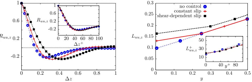
The rms of the three velocity components and the Reynolds stresses are shown in figure 3 for increasing values ofa
383
andb= 0.02. The value ofurms at the wall increases withaand the effect of the hydrophobic surface is to attenuate 384
the turbulence activity through the domain, confirming the main results by Min and Kim [4] for the
constant-slip-385
length case. The modification is strengthened asaincreases, which is consistent withRbecoming larger as the average
386
slip length increases. The streamwise velocity is the less affected, while the wall-normal and the spanwise velocities are
387
attenuated by the same amount. The Reynolds stressesuvreyare the most affected, with the peak decreasing by more 388
than 50%. Figure 4 shows theurms anduvrey scaled with the viscous units of the hydrophobic flow. Near the wall, 389
where the streamwise-velocity boundary conditions are altered, theurms display a marked differences, i.e., u+rms(0) 390
and the peak ofu+
rms grow withL as expected. The changes at higher wall-normal locations are less significant and 391
are thus mostly due to the modification of the Reynolds number. The collapse of the Reynolds stresses is confined
392
very near the wall.
393
It is paramount to verify that the cases studied above can be realized experimentally. The maximum Rcase is
394
considered, for whichL+0= 10.5. It is assumed that this scaled value corresponds toL∗
= 100µm, which is a sensible
395
choice according to several experimental and theoretical works [7, 8, 20]. From these values ofL+0 andL∗ the ratio
396
u∗
τ/ν∗ can first be found. Assuming the liquid to be water (ν∗=10−6 m2s−1), the channel height 2h∗ = 3.4mm and 397
the bulk velocityU∗
10
30
50
10
−810
−610
−410
−2R
(%
)
[image:14.595.182.418.84.245.2]a
b
= 0
b
= 0
.
01
b
= 0
.
02
FIG. 2: Comparison between theRvalues computed via DNS (white circles fora→0 and black circles for finitea) and the theoretical prediction obtained through the modified FKK formula (49) (lines).
0 4 8 12
0 0.1 0.2 0.3 0.4 0.5
ur
m
s
(
×
10
−
2)
y
no control
b= 0.02
a= 0.001, b= 0.02
a= 0.005, b= 0.02
a= 0.01, b= 0.02
0 1 2 3 4
0 0.1 0.2 0.3 0.4 0.5
vrm
s
(
×
10
−
2)
y
0 1 2 3 4 5
0 0.1 0.2 0.3 0.4 0.5
wr
m
s
(
×
10
−
2)
y
0 4 8 12
0 0.1 0.2 0.3 0.4 0.5
−
u
vr
ey
(
×
10
−
4)
y
[image:14.595.87.495.368.664.2]0 0.5 1 1.5 2 2.5 3
0 10 20 30 40 50 60 70 80 90 100
u
+ rm
s
y+
no control b= 0.02 a= 0.01, b= 0.02
0 0.2 0.4 0.6 0.8
0 10 20 30 40 50 60 70 80 90 100
−
u
v
+ rey
[image:15.595.90.494.78.213.2]y+
FIG. 4: Profiles of the rms of the streamwise velocity component (left) and of the Reynolds stresses (right), scaled with the viscous units of the hydrophobic flow.
fluid ν∗
(m2s−1) R
τ,r Rp 2h∗ (mm) Ub (ms−1)
water 10−6 180 4200 3.4 1.6
30% water+ glycerin 2.5×10⁻⁶ 180 4200 3.4 4.1
water 10−6 400 10400 7.6 1.8
30% water+ glycerin 2.5×10⁻⁶ 400 10400 7.6 4.6
water 10−6 1100 33060 20 2.1
30% water+ glycerin 2.5×10⁻⁶ 1100 33060 20 5.3
TABLE I: Estimates for the channel heights and the bulk velocities for different fluids and Reynolds numbers for
L∗
= 100µm andL+0= 10.5.
can be realized in a laboratory. Table I shows more estimated values for channel-flow experiments, where the same
399
slip lengths in viscous units and in physical dimensions are assumed (the empirical relationshipRp= 11.05R1τ,r.143was 400
used for the estimates at higher Reynolds numbers[55]). Our estimated flow quantities are comparable with those of
401
Rosenberget al.[15], who, for the first time, measured turbulent drag reduction (maximum R= 14%) in a Couette
402
flow over SLIPS. The friction Reynolds number was Rτ = 140, the maximum velocity was 4.4 m/s, and the gap 403
thickness was 2 mm. Although no information was reported on whether their slip length depended on the shear rate,
404
L∗=138
±55 µm (L+≈10) is comparable to ours and to Choi and Kim [8]’s.
405 406
A further comment is due on the results by Choi and Kim [8], shown in figure 1 (right). By extrapolating the
407
data, such surface would produce a slip length of 100µm when S∗
=450s−1. We compare these quantities with our
408
predictions in table I. For the first case in table I, b∗
=36µm is assumed, S∗
is about 10,000s−1 and a∗
=0.01µm s.
409
The shear rate is about 20 times larger Choi and Kim [8]’s and the constant of proportionality a∗ is one order of
410
magnitude smaller than Choi and Kim [8]’s. It follows that in a turbulent flow a much lower athan that found by
411
Choi and Kim [8] would lead to significant shear-dependent effects because the wall-shear stress is much larger. This
412
analysis proves that in wall-bounded turbulent flows, where the shear rate are orders of magnitude larger than in the
413
laminar flows, hydrophobic surfaces are likely to feature slip lengths with shear dependence.
414
Further evidence of shear-dependent slip lengths emerges from the recent DNS investigation by Jung et al. [37],
415
where turbulent channel flows atRτ,r = 180 over thin air layers have been simulated for the first time. Their figure 5f 416
demonstrates that the slip length depends on the wall-shear stress for high-drag-reduction cases with zero mass flow
417
rate in the air layer (refer to their figure 1b for a schematic of the flow domain). We have interpolated the data in
418
their figure 5f with a power law, i.e., u+0
s =aj(0.01µr∂u+0/∂y
y=0)
β, where µ
r is the ratio between the viscosities 419
of water and air. The least squares fitting method leads toaj = 0.006 andβ = 2.02. This means that for this type 420
of idealized hydrophobic surfaces our boundary condition (24) with b= 0 and a= 0.04 (computed by rescalingaj) 421
is a very good model relating the instantaneous streamwise slip velocity and the streamwise velocity gradient at the
422
water-air interface. According to our figure 2, this value ofawould lead toRabove 60%, which is consistent with the
423
wall-shear stress reduction computed by Junget al.[37]. It is certainly necessary to carry out further experimental and
424
modeling work for flows at high wall-shear stress, especially in the turbulent flow regime, in line with the numerical
[image:15.595.161.455.260.357.2]