The performance of the jet trigger for the ATLAS detector during 2011 data taking

DOI 10.1140/epjc/s10052-016-4325-0 Regular Article - Experimental Physics

The performance of the jet trigger for the ATLAS detector during

2011 data taking

ATLAS Collaboration CERN, 1211 Geneva 23, Switzerland

Received: 27 June 2016 / Accepted: 18 August 2016

© CERN for the benefit of the ATLAS collaboration 2016. This article is published with open access at Springerlink.com

Abstract The performance of the jet trigger for the ATLAS detector at the LHC during the 2011 data taking period is described. During 2011 the LHC provided proton–proton collisions with a centre-of-mass energy of 7 TeV and heavy ion collisions with a 2.76 TeV per nucleon–nucleon collision energy. The ATLAS trigger is a three level system designed to reduce the rate of events from the 40 MHz nominal max-imum bunch crossing rate to the approximate 400 Hz which can be written to offline storage. The ATLAS jet trigger is the primary means for the online selection of events containing jets. Events are accepted by the trigger if they contain one or more jets above some transverse energy threshold. Dur-ing 2011 data takDur-ing the jet trigger was fully efficient for jets with transverse energy above 25 GeV for triggers seeded randomly at Level 1. For triggers which require a jet to be identified at each of the three trigger levels, full efficiency is reached for offline jets with transverse energy above 60 GeV. Jets reconstructed in the final trigger level and correspond-ing to offline jets with transverse energy greater than 60 GeV, are reconstructed with a resolution in transverse energy with respect to offline jets, of better than 4 % in the central region and better than 2.5 % in the forward direction.

Contents

1 Introduction . . . . 1.1 The ATLAS detector and trigger system . . . . . 2 Jet trigger design overview. . . . 2.1 Level 1. . . . 2.2 Level 2. . . . 2.2.1 Level 2 data preparation . . . . 2.2.2 Level 2 jet reconstruction algorithm . . . . 2.2.3 Level 2 full scan trigger . . . . 2.3 Event filter. . . . 2.3.1 Event filter data preparation . . . . 2.3.2 Pile-up noise suppression. . . .

_{e-mail:[email protected]}

2.3.3 Jet finding and hypothesis testing . . . . . 3 The jet trigger menu . . . . 4 Timing . . . . 4.1 Level 1. . . . 4.2 High level trigger . . . . 5 Comparison of trigger and offline performance . . . . 5.1 Data samples and event selection . . . . 5.2 Jet trigger performance metrics . . . . 5.2.1 Efficiency definition . . . . 5.2.2 Trigger efficiency behaviour near threshold 5.2.3 Definition of transverse energy

resolu-tions and offsets. . . . 5.3 Transverse energy offsets and resolutions. . . . . 5.3.1 Central jets . . . . 5.3.2 Forward jets. . . . 5.3.3 The performance with respect to offline

EM scale jets . . . . 5.4 Jet trigger reconstruction efficiency . . . . 5.4.1 The single inclusive jet trigger efficiency . 5.4.2 Trigger efficiency versus pseudorapidity . . 5.4.3 The multi-jet trigger efficiency . . . . 6 Jet identification forppcollisions performed by

spe-cialised jet triggers . . . . 6.1 HTtriggers . . . . 6.2 Large-Rjet triggers . . . . 7 Jet identification for heavy ion collisions . . . . 7.1 Performance of the heavy ion triggers . . . . 8 Summary . . . . References. . . .

1 Introduction

ATLAS [1] is one of two general purpose detectors at the Large Hadron Collider (LHC) [2]. During the 2011 run-ning period the LHC operated with a collision energy of

√

centre-of-mass energy of 2.76 TeV for each pair of colliding nucle-ons in the interaction.

The large event rate at the LHC makes the online selec-tion of interesting physics events essential for achieving the physics goals of the LHC programme. During the 2011 data taking period, the LHC ran with a bunch spacing of 50 ns pro-viding a nominal rate of 20 MHz, and with a mean of more than 20 separateppinteractions per bunch crossing (known as pile-up) towards the end of data taking. To reduce the rate of events to be read out from the detector to a rate of around 400 Hz which can be written to offline storage, a rejection factor greater than 105is required. This is achieved by the ATLAS trigger [3] which is divided into the Level 1 (L1) trigger and the High Level Trigger (HLT). In 2011 the HLT itself consisted of two levels: Level 2 (L2) followed by the event filter (EF).

The jet trigger system of the ATLAS detector is the pri-mary means to select events containing jets with high trans-verse energy (ET). It selects collision events to be used in

jet physics analyses [4–11], as well as in many other anal-yses where one or more jets may be required, perhaps in conjunction with additional physics signatures such as an isolated lepton candidate. In this paper, the design and perfor-mance of the ATLAS jet trigger during the 2011 data taking is described.

The outline of this paper is as follows: Sect.2describes the design of the ATLAS jet trigger. Section 3 provides an overview of the jet based event selection defined in the ATLAS trigger menu and explains the nomenclature used for trigger names. The timing, or CPU budget, of each trig-ger level is outlined in Sect.4. Various aspects of jet trig-ger performance are described in Sect.5, which outlines the measures used for the evaluation of the trigger performance, and includes the selection efficiencies for inclusive single jet and multi-jet triggers. Descriptions of specialised trig-gers designed for specific physics selections are provided in Sect.6. These include selections for triggering on large summed scalarETor boosted objects that can decay into

mul-tiple narrow jets. Event selection in the Pb+Pb programme is described in Sect.7.

1.1 The ATLAS detector and trigger system

The ATLAS detector is a multi-purpose particle detector with a forward-backward symmetric cylindrical geometry and a near 4π coverage in solid angle.1Owing to the cylindrical

1_{ATLAS uses a right-handed coordinate system with its origin at the}

nominal interaction point (IP) in the centre of the detector and thez-axis along the beam pipe. Thex-axis points from the IP to the centre of the LHC ring, and they-axis points upwards. Cylindrical coordinates(r, φ)

are used in the transverse plane,φbeing the azimuthal angle around the

z-axis. The pseudorapidity is defined in terms of the polar angleθas η= −ln tan(θ/2).

geometry, subdetector components are described as being in thecentral region, if they are part of the barrel, at small abso-lute pseudorapidity, or described as forward, if part of the endcaps at large absolute pseudorapidity. Outwards from the beam pipe, ATLAS consists of an inner tracking detector sur-rounded by a thin superconducting solenoid providing a 2 T axial magnetic field, electromagnetic and hadronic calorime-ters, and a muon spectrometer. The inner tracking detector covers the pseudorapidity range|η|<2.5 and consists of sili-con pixel, silisili-con microstrip, and transition radiation tracking detectors.

The calorimeters cover the region |η| < 4.9 and con-sist of electromagnetic (EM), and hadronic subsystems. The EM, the hadronic endcap (HEC), and the forward calorime-ters (FCal) use liquid argon (LAr) as the active medium, and either a lead, copper or tungsten absorber technology. The EM calorimeter is divided into a barrel part,|η|<1.475, and two endcap components with 1.375 <|η| <3.2. The cen-tral hadronic calorimeter, referred to as the tile calorimeter, uses steel absorber layers interleaved with plastic scintillator covering the pseudorapidity range|η| <1.7. A presampler is installed in front of the EM calorimeter for|η|<1.8. For the calorimeter subsystems, there are two separate readout paths: the first, a very fast readout of combined towers of calorimeter cells, is used at Level 1, while the second is the slower readout of the full calorimeter cell information for use in the HLT and offline.

Event Filter 1800 PCs < t > ~ 4 s

Event Builder

processing HLT

Full Event Buffers Readout Buffers Requested Data in RoI

Access to full event

< 75 kHz

~ 3 kHz

~ 400 Hz ~ 600 MBs-1 Tracking

Detectors

Front End Pipelines Calorimeter,

Muon, Specialised Detectors

Level 1 Fast Custom Electronics t < 2.5 s

Level 2 500 PCs < t > ~ 40 ms

Fig. 1 The ATLAS trigger system

Following the L2 processing, all events with RoIs that satisfy a set of predefined selection criteria are passed to the event builder which reads out the detector at full granularity. These fully built events are then processed by the EF, which also consists of a farm of commodity CPUs. The EF farm runs modified versions of the offline reconstruction algorithms, simplified to improve the speed of execution. Although the full event data are available at the EF, for many trigger sig-natures the EF trigger reconstruction takes place within RoIs for reasons of speed. This is not the case for the jet trig-ger, for which the whole detector is read out. The rate of L2 accepted events passed to the EF during 2011 was approx-imately 3 kHz, and the rate at which events were read out for offline storage was approximately 400 Hz. The ATLAS trigger is illustrated in Fig.1.

In 2011 the full jet trigger was operated in rejection mode for the first time, allowing events to be discarded at each of the three trigger levels. Prior to 2011, the ATLAS trigger selection for events containing jets was based purely on the algorithms running at L1 and L2, with the EF algorithms executed in commissioning mode only. In this mode, events were processed by the EF but not rejected should they have failed the EF requirements. The resulting trigger decision was stored in the event stream for commissioning purposes.

2 Jet trigger design overview

The jet trigger is an integral part of the ATLAS trigger system, processing events based on successively more detailed detec-tor information at the L1, L2 and EF stages. Hadronic and electromagnetic energy deposits in the calorimeter subsys-tems are used to reconstruct jets; fast, custom jet algorithms are used at L1 and L2; and for the EF, the anti-kt [14]

algo-rithm in the four-momentum recombination scheme, imple-mented in theFastJet[15] package is used. In each of the three stages, the bandwidth allocated to the jet trigger is about 10 % of the total. Jet trigger signatures, simply referred to as jet triggers, are divided into eithercentralorforward, with the central jet triggers using detector data from the central and endcap calorimeters (|η|<3.2) and the forward jet trig-gers in the region 3.2<|η|<4.9 using data from the FCal. Different electronics are used for each to take account [16] of the more coarse FCal detector granularity in the forward direction.

The L1 calorimeter trigger system (L1Calo) [17], is the first stage of the jet trigger. This reconstructs jets from the combined energy deposits in the LAr and tile calorimeters, using collections of calorimeter cells projecting back to the nominal interaction point, known astrigger towers. A square sliding window of 0.8×0.8 inη×φis used to identify regions where the summed transverse energy within the cen-tral 0.4×0.4 region of the window is large and corresponds to a local maximum [18,19].

The jet candidateETvalues are then compared to a set of

predefinedETthresholds to decide which candidates should

form an RoI. The trigger thresholds are discussed in Sect.3. Information about the regions of the detector that contain jet candidates – specifically the multiplicity of candidates exceeding each threshold – is sent to the central trigger pro-cessor (CTP) and used in the generation of the global L1 decision. This is then distributed to the detector front-end electronics, to initiate the data readout, and the subsequent stages of the trigger. Information on which jet thresholds from L1 have been satisfied can also be combined with informa-tion from other L1 trigger subsystems, such as electron or muon triggers, to produce multi-object triggers.

found using the iterative cone algorithm are tested with a hypothesis algorithmto determine if they fulfil the prede-termined L2 trigger selection criteria. These criteria may include minimum values for the jet transverse energy, and selection on the jet pseudorapidity and quality. Each event selected at L2 is then fully built from the various fragments temporarily stored in memory in the data acquisition sys-tem.

The final stage of the trigger, the EF, must perform jet reconstruction in the full event within approximately 4 s before making a decision on whether to write the event to offline storage. Due to the larger available latency at the EF compared to L2, more sophisticated reconstruction algo-rithms can be applied. To the maximum extent possible, the EF uses standard ATLAS event reconstruction algorithms developed for offline analysis, as well as final offline detec-tor calibrations. Since the EF runs after the full event has been built by the event builder, it is able to access informa-tion from the complete detector, rather than just that from detector elements in an RoI. The EF jet trigger reconstructs anti-kt jets in the full calorimeter, in the same manner as

the standard offline jet reconstruction, rather than separately processing data within individual RoIs.

The ability of the EF to operate on the full calorimeter data permits seeding by triggers which select, at random, some fraction of events from L1 at a predefined rate irrespective of whether any RoI is present. Using the random trigger in this way allows the EF to trigger on jets free from any bias that might be introduced by the jet reconstruction at either the L1 or L2 stages. This is particularly useful for lowerET

jet thresholds, where such biases can be large.

2.1 Level 1

The L1 trigger decision is based on analogue sums of signals from calorimeter elements within 7168 projective regions (trigger towers), independent of the precision readout used in the HLT and offline. Trigger towers have a size of approx-imatelyη×φ = 0.1×0.1 in the central part of the calorimeter within|η|<2.5, and are larger and less regular in the more forward regions. Electromagnetic and hadronic calorimeters have separate trigger towers. The 7168 analogue inputs to the L1 calorimeter trigger are first digitised and then assigned to a particular LHC bunch crossing.

Two separate processor systems, working in parallel, run the trigger algorithms. One system, the cluster processor, uses the full L1 trigger granularity information in the central region to look for small localised calorimeter energy clusters typical of electrons, photons or the products of tau lepton decays. The other, used for jet and missing energy triggers, uses coarser granularityjet elements, to identify jet candi-dates and form global ET sums: missingET, totalET, and

the scalar sum of all jetET. The jet elements consist of 2×2

arrays of trigger towers in the central region and fewer in the foward region where the trigger towers are larger. TheETof

individual energy depositions and theETsums are compared

to preprogrammed trigger thresholds to form the trigger deci-sion. Jet RoIs are defined as 4×4 jet element windows for which the summed electromagnetic and hadronic calorime-terETexceeds predefined thresholds and which encompass

a 2×2 jet element core where the hadronic calorimeterET

is a local maximum. The location of the centre of this 2×2 array defines the coordinates of the jet RoI.

2.2 Level 2

In order to handle the large event rate from the detector, following a decision to accept an event at L1, the L2 deci-sion must arrive within approximately 40 ms. Even with the reduction in data volume from reading out only those data corresponding to the RoIs identified by L1, the data prepara-tion at L2 still represents a large contribuprepara-tion to the overall processing time. In this section the data preparation and jet finding stages of the L2 system are discussed.

2.2.1 Level 2 data preparation

The data preparation for the L2 jet trigger is a crucial part of the L2 processing. It provides the collection of data from detector readout drivers (RODs) [12], delivery to the L2 pro-cessing units, and the conversion from the raw data into the objects used by the HLT algorithms. The RODs receive data from the calorimeter front-end boards via optical fibres. These boards are installed on the detector and contain elec-tronics for the amplification, shaping, sampling, pipelining, and digitisation of the calorimeter signals [20,21]. Due to the large number of calorimeter readout channels, approximately 2×105_{, and in order to meet the L2 timing performance goal}

of 40 ms per event, the data volume read out should be kept to the minimum required to avoid compromising algorithm performance. For each detector element (calorimeter cell) within the RoI window, the direction from the nominal inter-action point to the element position is binned in a grid in the

η–φplane, for use in the L2 jet reconstruction algorithm.

2.2.2 Level 2 jet reconstruction algorithm

At L2, jets are defined as cone-shaped objects [16] in theη–φ plane with a given radius, R, such that they contain energy deposits with a separation R ≡ (η)2_+(φ)2 _{< R,}

• First, an initial reference jet, j0, is defined by the L1 jet

RoI position with the predefined cone radiusR. Note that the possible directions of the reference jet are discrete due to the 0.2×0.2 granularity at L1.

• The k elements from the binned distribution that fall within the (η,φ) region encompassed by the reference jet, j0, are used to recalculate the jet energy and the energy

weighted average position of the jet, to define a new, updated reference jet j1, according to

Ej1 = k

i=1

Ei, (1)

ηj1 =

k

i=1Eiηi

k

i=1Ei

, (2)

φj1 =φj0+

k

i₌1Ei×(φi−φj0)

k

i=1Ei

. (3)

where the sum runs over thekgrid elements whose cen-troids are contained within the cone of radiusRcentred on the reference jet j0. The total energy, and coordinates

ηj1andφj1, are computed from Eqs. (1), (2) and (3). • The previous step is repeated with j0replaced by j1in

Eqs. (2) and (3), and so on to form jet ji from jet ji−1,

updating the jet energy Eji and the coordinatesηji and φji. The iteration is repeatedNtimes to create jet jN. A configurable number of iterations are executed. Typically, N =3 is used, having been found sufficient to achieve the required performance [16].

The result of this algorithm is a jet defined by the recon-structed (η,φ) direction, and the total jet energy. This energy is evaluated at the electromagnetic calorimeter energy scale, by summing the energy depositions in the electromagnetic and hadronic parts of the calorimeter without applying any further calibration.

For the central jet trigger,R=0.4 is used. For the forward jet trigger, because of the coarse granularity of the FCal, the radii used for the first and second iterations are 1.0 and 0.7 respectively, to ensure that the energy deposits are fully contained given the coarse position available for the L1 jet. For the final iteration, the radiusR=0.4 is used.

2.2.3 Level 2 full scan trigger

Towards the end of data taking in 2011 a newLevel 2 full scan trigger [22,23], using the lower granularity trigger tower data from Level 1, was introduced. Here, the trigger tower data for the full calorimeter for each event was read out by the Level 2 system and processed on the Level 2 CPU farm with the anti-ktalgorithm. This trigger was running in commissioning

mode only during the heavy ion run at the end of 2011 and

was not deployed for production data taking in the proton– proton jet trigger until 2012.

2.3 Event filter

The EF is the last stage in the trigger and is responsible for the final decision of whether an event should be sent to offline storage or discarded. The jet trigger at the EF is modular and makes use of three general stages; data preparation (calorime-ter unpacking and pre-clus(calorime-tering), jet finding, and hypothesis testing.

In contrast to the RoI-based approach used at L2, the EF runs the jet finding algorithm once per event for each con-figured jet radius, using data from the complete calorimeter. This is referred to as afull scan. The full scan approach has several advantages for jet reconstruction with respect to the RoI based approach used at L2. The large RoIs required at L2 to ensure that any jet is completely contained has the unfor-tunate disadvantage that RoIs may overlap in events with high jet multiplicity, resulting in some parts of the detector being processed multiple times. This can result in jets being fully, or partially reconstructed in several RoIs, which may cause the double counting of energy deposits and jets, which would affect the multi-jet signatures. The full scan approach completely eliminates the multiple processing of regions of the detector and, as a consequence, leads to faster process-ing in high occupancy events, although it takes longer in low occupancy events, where the processing time is in any case low.

Since the output from L2 is in the form of lists of RoIs passing each trigger threshold, a slightly different approach is required to seed the EF processing. In this case, the first jet RoI to be processed by the EF initiates the creation of a dummy, full scan RoI, encompassing the entire detector, required to ensure that the entire calorimeter is processed. The calorimeter cell data for this full detector RoI is then extracted by the cell maker and processed to provide the objects upon which the jet finding will then run. Following the jet finding, hypothesis algorithms are executed. These determine whether any specific jet selection signatures are satisfied, for example, typical selections are those based on specific jetETthresholds.

The objects from both the data preparation and the jet find-ing stages are cached for this full scan RoI. When evaluatfind-ing any additional trigger signature requiring jets passing a dif-ferentETthreshold in the same event, the trigger can

estab-lish that this dummy RoI has already been created and will not start the sequence for the data preparation and jet finding again, instead simply retrieving the jets from the cache. The hypothesis algorithm for this differentETthreshold will then

be executed.

> 30 GeV ET > 40 GeV

Jet

ET > 100 GeV

Jet Hypothesis

Hypotheses

Jet reconstruction Jet reconstruction

Dummy RoI

Creator Cell Maker

Topological Clustering

Data preparation

anti-k Radius = 0.4

> 30 GeV ET > 40 GeV

Jet

ET > 100 GeV

Jet Hypothesis

Hypotheses

anti-k Radius = 1.0

t t

ET

ET

Fig. 2 The stages of algorithm processing in the Event Filter for several inclusive single jet triggers with differentETthresholds. The case illustrated

shows two sets of signatures, each set with a different jet radius parameter

run over the cached data and only the jet finding itself will be executed again for each different required radius. In this way the data preparation is common to all jet finding, which is in turn executed only once for each jet radius required. The full sequence for multiple thresholds and multiple jet radius parameters is illustrated in Fig.2and the individual stages are discussed in more detail below.

2.3.1 Event filter data preparation

The jet finder stage can operate with a number of differ-ent types of input objects produced by the data preparation from the raw cell data. In early 2011 the primary objects used as input to jet finding were projective calorimeter tow-ers constructed from the raw calorimeter cell information. From May 2011, so-called topological clusters [18] were used. These are discussed later. Since the offline jet recon-struction also uses topological clusters, this improves the EF jet resolutions with respect to offline reconstruction, although the topological clustering algorithm does add additional pro-cessing time to the data preparation stage.

The topological clustering algorithm creates clusters of topologically related energy deposits. The algorithm starts with a seed calorimeter cell, with an energy deposit with absolute value greater than four standard deviations above the expected noise. All cells directly neighbouring these seed cells, in all three dimensions, are collected into the cluster. Cells adjacent to the cluster are then added, if they have an energy with an absolute value exceeding the noise by two standard deviations, iterating until all such adjacent cells have been used. Finally, a ring of guard cells is added to complete the cluster. After the initial clusters have been formed, they

are analysed to identify local maxima, and split should more than one such maxima be found in a cluster [18].

2.3.2 Pile-up noise suppression

Jet reconstruction in the trigger is affected by the presence of pile-up interactions, which give rise to energy deposits in the calorimeter that are unrelated to the primary interaction of interest. The overlap of these energy deposits with those of the jets of interest can distort the reconstructed direction and ETof the jet. Due to the long integration time of the

calorime-ter electronics – up to 600 ns [1] – the detector response is also dependent on energy deposits arriving earlier or later than the nominal beam crossing. The size and likelihood of contributions due to pile-up depend on the number of inter-actions per bunch crossing. To account for this, the noise thresholds applied during the topological clustering process were tuned at the start of the 2011 running period to reflect the expected mean number of interactions per bunch cross-ing.

2.3.3 Jet finding and hypothesis testing

Jet finding can be performed using any of the available offline jet algorithms. Due to problems with the infrared and collinear safety of cone algorithms [24], ATLAS has adopted k_⊥-ordered sequential combination algorithms [25,26], and specifically the anti-kt[14] algorithm in the four-momentum

recombination scheme as the jet algorithm of choice for physics analyses [4–6,8]. To match this offline choice, the anti-kt algorithm was chosen for use in the EF for 2011

algo-rithm used in the trigger prior to 2011. Two different values of the radius parameter,R, were used in the EF trigger recon-struction in 2011, R =0.4 and 1.0, the larger radius being useful for the study of hadronic decays of boosted heavy particles.

Should any additional calibrations be required for the final jets themselves, the jet reconstruction process can run a post-processing stage to apply them to jets. As in the case of the offline processing, the EF jet algorithm runs on the full calorimeter information. Differences between the trigger and offline jets generally only arise because the final offline cal-ibrations are not normally available at the time of data tak-ing. During the 2011 data taking the jet trigger was oper-ated at the electromagnetic scale, i.e. with no jet calibration applied.

For an inclusive single jet trigger, the hypothesis algo-rithm that executes following the jet finding, accepts events which have at least one jet which satisfies the required crite-ria. Since the jets for each event are cached in memory, subse-quent calls to hypothesis algorithms with different selection thresholds simply use this cached jet collection. Identify-ing multi-jet events is also simply a case of iteratIdentify-ing over the reconstructed jets to identify combinations which pass the relevant selections for each signature. Different multi-jet signatures are possible, including those where theETof each

jet in the event is required to exceed a differentETthreshold.

The hypothesis algorithm takes as parameters the required jet multiplicity,n, theηrange within which the jets must lie,

ηmin ≤ |ηjet| < ηmax, and the required ET thresholds for

each of the requirednjets.

3 The jet trigger menu

The trigger system is configured via a menu which includes the specification of the list of event signatures to be accepted for events written to offline storage. For the jet trigger, this includes the number of jets, ET thresholds, η ranges, and

other parameters such as jet-quality criteria, to be applied at each of the three trigger levels. The aim of the menu design is to deploy a complementary and robust set of selections for physics channels of interest, compatible with the given bandwidth limitations. The trigger menu determines the con-figuration of the L1 firmware and the algorithms executed at the HLT. Corresponding triggers in each of the three trigger levels constitute a triggerchain.

The names of the trigger selections used in this document consist of the jet multiplicity followed by theETthreshold

separated with ajfor L2 and the EF, or Jfor L1. This is preceded by the trigger level separated by an underscore, so for instanceEF_j100would be a 100 GeV single-jet trigger at the EF, andL1_5J10 would be a five jet trigger at L1 with a 10 GeV transverse energy requirement on each jet.

Addi-tional items may be included in the name for specialised trig-gers, such asFJfor forward jets which are required to have

|η| > 3.2. Typically the item names also include informa-tion regarding the specific jet algorithm. For instance a4tc or a10tcindicate that the anti-kt algorithm was used, with

radius parameters 0.4 or 1.0 respectively, and running on topological clusters (tc). Where this string is omitted, anti-kt jets with radius parameter R = 0.4 should be assumed.

All the jet triggers used at the EF during 2011 were full scan triggers, and as such had names appended byEFFSto indicate the EF full scan; however, for the following discus-sion, the EFFSmay be omitted from the trigger name for brevity.

Trigger selections at each level are designed to reduce the CPU usage at later trigger levels by maximising event rejec-tion at early stages. Trigger thresholds in the higher levels are tightened to avoid the distortion of the efficiency curve from the slower-rising efficiency of previous levels. Trig-gers can operate inpass-through mode, which entails exe-cuting the trigger algorithms but accepting the event irre-spective of the algorithm decision. This allows the trigger selections and algorithms to be validated, to ensure that they are robust against the varying beam and detector conditions, which are hard to predict before data taking. Partial pass-through mode allows only a certain percentage of events to be passed through the trigger in this way, the rest being sub-ject to the usual trigger selection. This operational mode was used during data taking for several triggers. Passing events through in this way allows data to be collected by the higher threshold triggers for performance evaluation and debugging, with as little bias as possible.

Further flexibility is provided by definingbunch groups, which allow triggers to include specific requirements on the LHC bunches colliding in ATLAS. Not all bunch crossings contain protons; those that do are calledfilledbunches. For the random trigger, filled bunch crossings were required, indi-cated in the trigger name byFILLEDat L1, andfilledat L2. Non-collision triggers require a coincidence with anempty orunpairedbunch crossing, which correspond respectively to no protons in either LHC beam or a filled bunch in only one beam. For some of the lowest threshold physics trig-gers, a corresponding non-collision trigger was included in the chain for background studies.

As well as the trigger chains selecting jets at both L1 and L2, there were chains running at the EF, which were seeded by a random trigger at L1, and passed the events through L2 without running a selection algorithm. These allowed trig-gering on very lowETjets at the EF without the biases

intro-duced by the L1 jet reconstruction at lowET.

Day in 2011 28/02 02/04 05/05 08/06 11/07 14/08 16/09 20/10 22/11

]

-1

s

-2

cm

33

Peak Luminosity per Fill [10

0 0.5 1 1.5 2 2.5 3 3.5 4

4.5 Online Luminosity s = 7 TeV LHC Stable Beams

-1

s

-2

cm

33

10

×

Peak Lumi: 3.65

(a)

Day in 2011 28/02 30/04 30/06 30/08 31/10

]

-1

T

o

tal Inte

gra

ted L

u

m

in

o

sity [fb

0 1 2 3 4 5 6

7 Online Luminosity s = 7 TeV LHC Delivered

ATLAS Recorded

-1

Total Delivered: 5.61 fb

-1

Total Recorded: 5.25 fb

(b)

Fig. 3 The luminosity measurement at the ATLAS interaction region

for 2011 data taking [29]:athe maximum instantaneous luminosity versus day delivered to ATLAS during stable beam operation;bthe cumulative luminosity versus day delivered to (green), and recorded by (yellow) ATLAS during stable beam operation for ppcollisions at 7 TeV centre-of-mass energy

• Event Filter triggers that reconstructHT, the total scalar

sum ofETof all jets in an event. Such triggers are useful

for physics analyses which study or search for events with a large summedETin the final state, as the requirement

of largeHTcan help to control the trigger rate without

requiring e.g. a very energetic leading jet;

• jet triggers where the jet algorithm is executed with a large-Rparameter, useful for searching for heavy parti-cles decaying into boosted hadronic final states; the anti-kt algorithm was used withR=1.0 (denoteda10); • heavy ion triggers, used for the Pb+Pb data taking period

at the end of 2011, having a total transverse energy requirement in GeV denoted byTE, differing with respect to the HTrequirement used in proton runs in that TE is

the sum of all transverse energy in the calorimeter, not only of that clustered in jets.

The first time ATLAS used both the L2 and EF stages of the HLT in event rejection mode was in 2011. A number of key improvements were introduced during that year, including the ability to use topological clusters rather than calorimeter towers at the EF, as discussed in Sect.2.3.1, which was found to increase the stability of the algorithm in the presence of pile-up. During the 2011 data taking period the LHC peak instantaneous luminosity increased by more than an order of magnitude, from 1032_cm−2_s−1_{to 3.6×10}33_cm−2_s−1_.

Figure3shows the maximum instantaneous luminosity and the integrated luminosity delivered to ATLAS during 2011 as a function of time. The highest values for the mean num-ber of interactions per bunch crossing reached∼20 towards the end of running in 2011. The jet trigger menu evolved during this period to adapt to the changing LHC condi-tions.

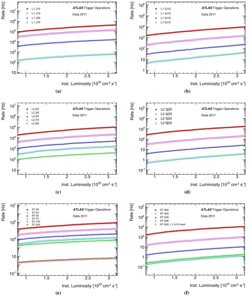
In order to keep the rate from the jet trigger within the allowed bandwidth, prescale factors are used to suppress the rates from signatures with lower thresholds. A prescaled trigger selects only a fraction, 1/prescale, of events that would otherwise pass the trigger. For the best expected sta-tistical significance, wherever possible, triggers intended for searches or analyses requiring the highest possible number of data events, should not be prescaled. As the luminos-ity increased during 2011 data taking, the prescale factors applied to the triggers with lower thresholds were increased accordingly, to ensure that the output rate remained within the available bandwidth for writing to offline storage. Figure 4 illustrates the evolution of jet trigger rates with instanta-neous luminosity for a selection of single inclusive jet and multi-jet triggers operating in 2011 at each of the three trig-ger levels. The rates shown are before application of any prescales. Typical prescale factors for the inclusive jet signa-tures applied on two separate dates during 2011 can be seen in Table1.

In addition to applying prescale factors to low-threshold triggers, the EF ETthreshold of the lowest-ETunprescaled

] -1 s -2 cm 33 Inst. Luminosity [10

1 1.5 2 2.5 3

Rate [Hz] 10 2 10 3 10 4 10 5 10 6 10 7

10 L1 J10_{L1 J15}

L1 J30 L1 J75

Trigger Operations

Data 2011

(a)

] -1 s -2 cm 33 Inst. Luminosity [10

1 1.5 2 2.5 3

Rate [Hz] 1 10 2 10 3 10 4 10 5 10 6 10 L1 3J10 L1 4J10 L1 5J10 L1 6J10 Trigger Operations Data 2011 (b) ] -1 s -2 cm 33 Inst. Luminosity [10

1 1.5 2 2.5 3

Rate [Hz] 10 2 10 3 10 4 10 5 10 6 10 7 10 L2 j25 L2 j35 L2 j50 L2 j70 L2 j95 Trigger Operations Data 2011 (c) ] -1 s -2 cm 33 Inst. Luminosity [10

1 1.5 2 2.5 3

Rate [Hz] -1 10 1 10 2 10 3 10 4 10 5

10 L2 3j25

L2 4j25 L2 5j25 L2 6j25

Trigger Operations

Data 2011

(d)

] -1 s -2 cm 33 Inst. Luminosity [10

1 1.5 2 2.5 3

Rate [Hz] -1 10 10 3 10 5 10 7 10 EF j30 EF j40 EF j55 EF j75 EF j100 EF j240 Trigger Operations Data 2011 (e) ] -1 s -2 cm 33 Inst. Luminosity [10

1 1.5 2 2.5 3

Rate [Hz] -1 10 1 10 2 10 3 10 4 10 5

10 _{EF 3j30}

EF 4j30 EF 5j30 EF 6j30 EF 6j30, L1 5J10 seed

Trigger Operations

Data 2011

(f)

Fig. 4 The jet trigger rates versus instantaneous luminosity, before application of prescale factors, for triggers operating in 2011a,c,efor several

Table 1 Typical values for the L1 and HLT prescales for the inclusive jet signatures, here denoted by the EF signatures, on two dates from different running periods. Also shown is the effective full chain prescale obtained by multiplying the L1 and HLT prescales. The three lowestETsignatures are seeded

by a random trigger at L1 with the same prescale, but have separate prescales at the HLT to control the rate. The remaining signatures are seeded by a jet trigger at both L1 and L2

Apr 28th _{Oct 22}nd

Trigger L1 prescale HLT prescale Combined L1 prescale HLT prescale Combined

EF_j10_a4tc† _{2 710 60.9 165 039 58 600 18.6 1 089 960}

EF_j15_a4tc† _{2 710 12.4 33 604 58 600 4.3 251 980}

EF_j20_a4tc† _{2 710 3.8 10 298 58 600 1.2 70 320}

EF_j30_a4tc 7 550 1 7 550 39 300 1 39 300

EF_j40_a4tc 5 080 1 5 080 25 300 1 25 300

EF_j55_a4tc 1 110 1.3 1 443 3 940 1.8 7 092

EF_j75_a4tc 404 1 404 1 910 1 1 910

EF_j100_a4tc 1 116 116 1 529 529

EF_j135_a4tc 1 3 3 1 135 135

EF_j180_a4tc 1 1 1 1 31.6 31.6

EF_j240_a4tc 1 1 1 1 1 1

EF_j320_a4tc‡ _{1 1 1}

EF_j425_a4tc‡ _{1 1 1}

†_{Randomly seeded at L1, passthrough at L2} ‡_{Not active during early running}

Table 2 The evolution of the lowestET, unprescaled EF threshold for

single-jet triggers during 2011 data taking Instantaneous Luminosity

[1033cm−2s−1]

Lowest unprescaled trigger

ETthreshold [GeV]

0 – 0.16 100

0.16 – 0.25 135

0 8 1 1

. 1 – 5 2 . 0

1.1 – 3.6 240

4 Timing

As a hardware system, the L1 trigger operates with a fixed latency, whereas the L2 and EF systems operate with a vari-able processing time, and must complete their respective pro-cessing within the constraints provided by the L1 rate, the rate at which events can be recorded offline, and the number of available CPU nodes in each HLT farm. In this section, the time taken to process events for the L1 system and the HLT is discussed.

4.1 Level 1

The L1 jet trigger is a fixed latency, hardware based trigger operating synchronously with the LHC bunch clock and the rest of the L1 system. The pipelines in the detector front-end electronics are typically 120 bunch crossings deep and as such the latency from the complete L1 processing must fit within the corresponding time. Throughout the L1 system each step is handled in parallel with other steps. Data trans-fers between parts of the system are performed concurrently with the processing of the data that has already been

trans-ferred. The analogue data are digitised and sent as input to a jet algorithm, and the final decision is sent from the L1 calorimeter system to the central trigger processor (CTP). The jet algorithm processing itself is very fast and takes only approximately 50 ns, but represents only part of the process-ing necessary to reconstruct jet candidates, the rest beprocess-ing in formatting the input and output data such that the algorithm can execute quickly. The overall time for all these stages including the transmission of the results of the calorimeter trigger reconstruction to the CTP is approximately 1.5µs. The additional time required for the subsequent CTP pro-cessing to determine the global L1 decision, and the time taken for transmission of this decision back to the detec-tor front-end is approximately 0.5µs so that the full latency of the entire L1 system is within the required maximum 2.5µs.

4.2 High level trigger

pro-Algorithm time [ms]

0 20 40 60 80 100

]

-1

Dif

ferential counts [ms

1 10

2

10

3

10

4

10 _ATLAS

ata 2011

Level 2 jet reconstruction

< t > = 13.8 ms : per event

< t > = 6.5 ms : per RoI

(a)

Algorithm time [ms]

0 20 40 60 80 100

]

-1

Dif

ferential counts [ms

1 10

2

10

3

10

4

10 ATLAS

ata 2011

Level 2 jet reconstruction

< t > = 8.0 ms : per event

< t > = 3.7 ms : per RoI

(b)

Algorithm CPU time [ms]

0 5 10 15 20 25

]

-1

Dif

ferential counts [ms

10

2

10

3

10

4

10 ATLAS_{ata 2011}

Level 2 jet reconstruction

< t > = 5.9 ms : per event

< t > = 2.8 ms : per RoI

(c)

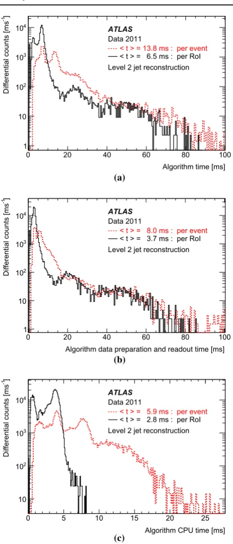
Fig. 5 The processing time for the L2 jet trigger:athe full algorithm

time;bthe data preparation time;cthe algorithm processing CPU time. The full algorithm time includes both the data preparation and algorithm processing times. Thesolid linesshow the processing time per call, and thedashed linesshow the processing times per event

cessing mean time of 2.8 ms and a combined data preparation and readout time with a mean of 3.7 ms which also provides the long tail.

The execution time of the algorithm per event, rather than per RoI shows a clear peak around 6 ms and a second peak around 12 ms, due to events containing two RoIs. The data preparation time for the full event has a peak at around 3 ms for single RoI events and another from the two-RoI events around 6 ms. The algorithm CPU time has corresponding peaks around 4 and 8 ms.

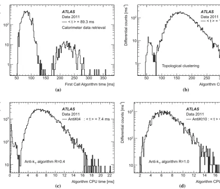
At the EF, following the data preparation steps – the retrieval of calorimeter cell information from memory and building of topological clusters – a single instance of the anti-ktjet finder is executed for each of the required jet radii,

R=0.4 andR=1.0. The times for each of the data prepa-ration stages and the two jet radii are shown in Fig. 6, for the same 2011 run. For the data retrieval stage, before the topological clustering, two distinct peaks are observed. The first, with a mean around 80 ms, represents the processing of the complete event. The second broader peak, with a mean of approximately 220 ms, is due to an artefact of the trigger processing by the EF farm: each CPU in the EF farm runs a separate instance of the EF software and performs some addi-tional initialisation for the first event each receives, increas-ing the processincreas-ing time for the first event processed by each CPU node. The number of events in this second peak then corresponds to the number of individual CPUs in the farm. The most time consuming part of the full EF processing is the topological clustering, with a mean of approximately 170 ms. The jet finding itself is comparatively fast, requiring approx-imately 7 ms per instance. Due to the different prescales and thresholds used for the triggers for the different jet radii, the event topology andETspectrum is slightly different for

the events processed by each instance of the anti-kt

algo-rithm, resulting in the slightly different distributions seen in Fig. 6c, d. The peaks seen at short times in the topologi-cal clustering and R = 0.4 anti-kt jet finding are due to

the low threshold EF triggers seeded by the random trigger at L1 which therefore may contain fewer calorimeter cells with significant energy and so do not take as long to process. The anti-kt jet finding usingR=1.0 only processes events

seeded by jets found both at L1 and L2, where these jets pass the 95 GeV L2 threshold, so this peak is largely absent in Fig.6d.

After the jet finding has completed, the selection hypoth-esis algorithms are executed both at L2 and the EF. For the single inclusive and multi-jet triggers the hypothesis algo-rithm typically executes in approximately 10 µs for each signature.

5 Comparison of trigger and offline performance

First Call Algorithm time [ms] 50 100 150 200 250 300 350

]

-1

Dif

ferential counts [ms

1 10 2 10

ATLAS

ata 2011

Calorimeter data retrieval < t > = 89.3 ms

(a)

Algorithm CPU time [ms] 50 100 150 200 250 300 350

]

-1

Dif

ferential counts [ms

1 10 2 10

ATLAS

ata 2011

Topological clustering

< t > = 169.6 ms

(b)

Algorithm CPU time [ms] 0 2 4 6 8 10 12 14 16 18 20 22

]

-1

Dif

ferential counts [ms

10 2 10

3 10

ATLAS

ata 2011

algorithm R=0.4 T

Anti-k

AntiKt4 : < t > = 7.4 ms

(c) Algorithm CPU time [ms]

2 4 6 8 10 12 14 16 18 20

]

-1

Dif

ferential counts [ms

10 2 10

3

10 ATLAS

ata 2011

algorithm R=1.0 T

Anti-k

AntiKt10 : < t > = 7.0 ms

(d)

Fig. 6 The processing times for the Event Filter jet trigger:athe time

for the data preparation for the full calorimeter data;bthe process-ing time for the topological clusterprocess-ing;c,dthe times for the actual jet

finding for the anti-ktalgorithm, for instances with radius parameters cR=0.4, anddR=1.0

later reconstructed offline, to allow informed event selection with high efficiency while minimising any increase in the trigger rate. This is achieved by reducing any finite trigger– offline resolution or bias so that any selection of objects on the basis of trigger quantities more closely corresponds to the offline selection used for physics analyses. For this reason, the performance of the jet trigger during 2011 data taking has been evaluated with respect to the offline jet reconstruc-tion. The offline reference jets have been reconstructed using the infrared and collinear safe anti-kt algorithm [14]

imple-mented in the FASTJET [15] package. The same values of the radius parameter are used offline:R =0.4 for the stan-dard analyses, andR=1.0 used for the analysis of boosted objects.

The trigger performance is defined in terms of specific metrics, comparing offline and trigger reconstructed jets, such as jet selection efficiency, and the transverse energy or angular resolution with respect to offline jets. Comparisons

of the same metrics with Monte Carlo simulated samples are shown in this and the following sections to illustrate how well the simulation describes the data and where disagreements appear. It should be emphasised, however, that the focus is on performance indicators determined from collision data, and detailed comparisons of different simulation configurations are beyond the scope of this paper.

5.1 Data samples and event selection

kine-matics, hadronisation, treatment of underlying event, or to differences in the simulation of the detector response or the detector conditions.

Because of these potential sources of differences between data and simulation, for jet physics analyses, trigger selection and trigger related calibrations are generally obtained using the data rather than relying on the trigger performance from the Monte Carlo simulation. Therefore, while it is desirable for the simulation to accurately reproduce the behaviour of the trigger, it is by no means essential.

For the evaluation of the trigger performance, events are selected from those written offline that are free from known problems with the detector or beam conditions. From these events, offline reconstructed jets which satisfy standard ATLAS jet selection criteria used in physics analyses [4– 6] are selected to provide a reference jet sample. Besides the kinematic selection, these criteria also include jet-quality selections [10,30,31] to reject fake jets reconstructed from non-collision signals, such as beam-related background, cos-mic rays or detector noise. Similar jet quality criteria are applied online to the trigger jets.

The efficiency for each specific chain has been evaluated using events selected by an alternative chain which is unbi-ased by the selection of the chain being evaluated. There-fore, wherever possible, the efficiencies have been evaluated using trigger chains seeded by a random trigger at L1, pass-ing through L2 and EF without additional trigger selection. Where this was not possible, the standard chains have been used, but selecting only thosepass throughevents, where the trigger accepted the event irrespective of the trigger jet selection, as discussed in Sect.3.

There are a number of general purpose event genera-tors for LHC physics: for more complete review, see else-where [32]. In the following studies, data are compared with simulated events produced using either theHerwig[33] or

Pythia_{[34] Monte Carlo generators. Each simulates}

com-plete physics events using a hard subprocess with a leading logarithmic parton shower followed by a soft hadronisation model to generate the outgoing hadrons. Both include mod-els for the underlying event: InHerwig, the formation of hadrons from the final state quarks and gluons produced in the parton shower is described using a cluster hadronisation model [35], whereas thePythia generator uses the Lund string fragmentation model [36,37].

In the following discussion the central and the forward jets triggers are discussed separately. For central jet triggers in the range|ηjet|<3.2, offline jets are required to lie in the range |ηjet| <2.8 in order to completely contain jets with radius parameter 0.4. Similarly, for the forward jet triggers, which lie in the range 3.2 < |ηjet| < 4.9, offline jets satisfying 3.6<|ηjet|<4.5 are required.

For offline analyses, jets are corrected for the differ-ence between electromagnetic and hadronic responses in the

calorimeter. Therefore jets can be defined either at the elec-tromagnetic (EM) scale, which correctly measures the energy deposited by electromagnetic showers in the calorimeter, or after the full hadronic jet energy scale (JES) calibra-tion [31,38]. In the trigger, the JES calibration was not applied in 2011 since the full calibration was not available during data taking. The standard calibration of the reference offline jets is referred to as EM+JES, meaning jets built from (electromagnetic-scale) topological clusters, with jet energy corrected by the application of the JES calibration.

5.2 Jet trigger performance metrics

Descriptions of the metrics used to assess the jet trigger per-formance can be found in this section: specifically for the efficiency measurement, and the evaluation of the resolu-tion and bias arising from any offset between the trigger and offline reconstructed quantities.

5.2.1 Efficiency definition

Unless otherwise stated, the inclusive single jet efficiencies presented in this paper are of the form ofper jetefficiencies with respect to the corresponding jet reconstructed offline. This represents the probability that an offline jet will have a corresponding jet reconstructed in the trigger that satisfies the trigger selection. Efficienciesper eventcan also be defined, in terms of global event properties, such as the ET of the

leading jet in the event. These are more sensitive to the event topology and more difficult to interpret, since, for example, any other jet might cause the event to be accepted, even if the leading offline jet does not. For a multi-jet trigger however, where the selection depends on the properties of many jets, theseper eventselections may be very informative; this is discussed further in Sect.5.4.3.

The jet reconstruction efficiency,ε, for a sample of jets can be defined as the ratio of the number of offline jets, N, passing some selection which defines the sample, and the number of those jets,m, which are also reconstructed in the trigger to within some appropriate matching criteria, such thatε≡m/N.

The choice of matching criteria must be considered as an important aspect of the definition of the efficiency, since a tighter matching will necessarily result in a lower efficiency andvice versa. This is important since the correspondence of offline jets to trigger jets is not one-to-one.

The binned differential efficiency,εi, in some generic

vari-able xjet, where xi ≤ xjet < (xi +x), is defined

analo-gously,

εi =

m(xi ≤xjet< (xi +x))

N(xi ≤xjet < (xi+x)).

R(L1-Offline)

Δ

0 0.05 0.1 0.15 0.2 0.25 0.3 0.35 0.4 0.45 0.5

R Δ / d jets ) dN jets (1/N -3 10 -2 10 -1 10 1 10 Data 2011

> 60 GeV

Offline T

L1_J10: p

> 80 GeV

Offline T

L1_J15: p

> 100 GeV

Offline T

L1_J30: p

> 130 GeV

Offline T

L1_J50: p

> 160 GeV

Offline T

L1_J75: p

ATLAS

√s = 7 TeV

(a)

R(L2-Offline)

Δ

0 0.05 0.1 0.15 0.2 0.25 0.3

R Δ / d jets ) dN jets (1/N -3 10 -2 10 -1 10 1 10 2 10 R(L2-Offline) Δ

0 0.01 0.02 0.03 0.04 0.05

R Δ / d jets ) dN jets (1/N 0 20 40 60 80 100 120 140 160 180 ATLAS Data 2011

> 60 GeV Offline T L2_j25: p

> 80 GeV Offline T L2_j35: p

> 100 GeV Offline

T L2_j50: p

> 130 GeV Offline

T L2_j70: p

> 160 GeV Offline T L2_j95: p (b) R(EF-Offline) Δ

0 0.02 0.04 0.06 0.08 0.1 0.12 0.14 0.16 0.18 0.2

R Δ / d jets ) dN jets (1/N -3 10 -2 10 -1 10 1 10 2 10 3 10 R(EF-Offline) Δ

0 0.01 0.02 0.03 0.04 0.05

R Δ / d jets ) dN jets (1/N 0 50 100 150 200 250 300 350 ATLAS Data 2011

> 60 GeV Offline T EF_j30: p

> 80 GeV Offline T EF_j40: p

> 100 GeV Offline

T EF_j55: p

> 130 GeV Offline

T EF_j75: p

> 160 GeV Offline

T EF_j100: p

(c)

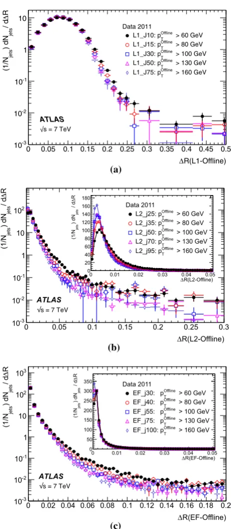
Fig. 7 The distribution ofRbetween the offline jets and the closest

matching trigger jet:afor L1;bfor L2;cfor the EF. In each case the differences are shown with respect to offline jets above thepT

thresh-olds indicated such that the trigger for each threshold is fully efficient. Statistical uncertainties only are shown

The criterion applied here for matching online and offline jets is based on the distanceR=(η)2_+(φ)2_{in the}

η–φplane between the offline jet and the closest matching trigger jet.

Figure7shows the distribution ofRfor trigger jets from L1, L2 and the EF. Distributions are shown for each trigger for several different pTranges such that the trigger in each

case is fully efficient. For the L2 and EFRdistributions, the agreement between online and offline clearly improves with increasing jetET. Since the L1 trigger uses only coarse

granularity calorimeter information, and quantises theηand

φdirections to the nearest 0.2, the resolution inηorφfrom L1 would be expected to be approximately 0.06. For similar Gaussian distributed residuals inηandφthis would result in a maximum in the R distribution of around 0.08, as observed in Fig.7a. Although the L2 trigger operates only within each RoI, it uses calorimeter information at the full detector granularity. Therefore the jetηandφreconstruction in Fig. 7b for L2 is significantly improved with respect to that seen in Fig.7a for L1. The EF uses the same topological clustering algorithm and the same jet finding algorithm as the offline reconstruction. This leads to a further improvement in the resolution between the trigger and offline jets for the EF with respect to what is already acheived at L2, and can be seen in Fig.7c.

For the matching used to define the resolution and effi-ciency, criteria inR have been chosen which allow high efficiency for genuine matches while reducing the contribu-tion from random matches that may degrade the resolucontribu-tion. For the analyses of the efficiency and resolution for single jets presented here, trigger jets are required to match with the closest offline jet to withinR <0.4 at L1, and to within

R<0.2 for L2 and the EF.

5.2.2 Trigger efficiency behaviour near threshold

The trigger system selects jets based largely on the ETand

pseudorapidity of the jets reconstructed at the three trigger levels. The principle source of difference between theETof

offline and trigger jets in 2011 was the hadronic calibration, which was not applied online in this period. Smaller differ-ences at the different levels arise from the detector granularity at L1, the input objects to the jet algorithms and the L2 algo-rithms. These differences give rise to shifts and additional resolution smearing of the ET reconstructed in the trigger

with respect to that reconstructed offline. The selection effi-ciencies for the various trigger levels resulting from these shifts and smearing are therefore not step functions when measured as a function of the offline ET. Instead, the

effi-ciency as a function ofETwill exhibit a more slowly rising

edge as the trigger turns on. This has an impact on ATLAS physics analyses; in general, a steeply rising efficiency near the ET threshold which rapidly approaches a plateau near

it has the potential to introduce large systematic uncertainties in the selection efficiency and background estimates.

A more slowly rising edge is expected at L1 due to the poorer ET resolution, arising from the coarse granularity

data. Care must therefore be taken to ensure that the L1 effi-ciency reaches its plateau forETvalues below the onset of the

rising edges of the L2 and EF efficiency curves. The thresh-olds for the higher trigger levels therefore impose upper limits on the corresponding L1 thresholds, and so reduce the effi-cacy of raising these thresholds in order to reduce the rate of L1 accepted events. Because of the steeply fallingpT

spec-trum this implies that more events need to be accepted at L1 to avoid reducing the EF efficiency significantly at higher ET. A more steeply rising efficiency is expected at the EF

due to the improvedETresolution and the greater similarity

in the reconstruction algorithms used online and offline. To minimise systematic uncertainties associated with the trigger, most ATLAS physics analyses relying on jet triggers require that the offlineETfor selected jets lie in theefficiency plateau

region, where the efficiency is above 99 %.

5.2.3 Definition of transverse energy resolutions and offsets

The transverse energy resolutions and offsets are computed from the distributions of the residuals between the quantities computed offline and at trigger level.

To provide a single statistic to parameterise the resolution, the root-mean-square (RMS) deviation of the central 95 % of the residual distribution is used. This is further divided by the RMS for the central 95 % of a Gaussian distribution with unit standard deviation. In this way, if the distribution were Gaussian, the normal Gaussian resolution would be obtained. This measure was chosen because the RMS of the full dis-tribution can be strongly biased by significant non-Gaussian tails. Similarly, a measure for the resolution based on the width of a Gaussian distribution fitted over the central region of the distribution will fail to take into account a significant fraction of the distribution if there are large tails and will not be representative of the actual performance.

Offsets and resolutions between jets reconstructed in the trigger and reconstructed offline are obtained from the dis-tribution of the quantity

E_TTrigger−E_TOffline

E_TOffline . (5)

For a comparison of offline, fully calibrated, jets with the trigger jets reconstructed at the electromagnetic scale, the transverse energy offset will be large. Therefore, results are first presented in terms of the jet definitions actually used by offline analyses and the online systems, and then also shown for the case of comparison of the online jets with the offline

jets, both reconstructed at the electromagnetic scale, which more closely resemble each other.

5.3 Transverse energy offsets and resolutions

Understanding of the offsets and resolutions in the data is useful for the determination of the behaviour of the trigger efficiencies near the ETthresholds, since the offset and

res-olution will, respectively, have an impact on the position and gradient of the rising edge.

As the resolutions and offsets presented in this section are with respect to offline jets at the EM+JES scale, large offsets are expected. For brevity, only the performance of the EF trigger is presented as this corresponds most closely to the offline reconstruction. Since physics analyses generally use pT, where applicable, the offset and resolution of the quantity

actually reconstructed in the trigger – namelyET– are shown

as a function of the offline jetpT.

In order to ensure that the trigger has reached plateau effi-ciency for the lowest L1 jet ETthreshold, the performance

in terms of reconstruction of the jet transverse energy and pseudorapidity is presented for offline jets withpT>60 GeV

when evaluating the central jet triggers seeded by the L1 jet trigger, and pT >50 GeV when evaluating the forward jet

trigger.

5.3.1 Central jets

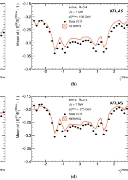
Figure8shows the mean relative offset as a function of the offline jetηfor both the data and theHerwigsimulated sam-ple integrated over pTabove four different thresholds,

indi-cated in the figure. The general trend of the data is reasonably well reproduced by the Monte Carlo simulation, with small differences at the percent level. As discussed previously, dif-ferences between the simulation and data result from inac-curacies or approximations in the simulation of the detector response or in the application of the detector conditions, but also from differences in the underlying kinematics and pT

spectrum of the Monte Carlo sample.

A largeηdependence can be discerned: at low pT,

neg-ative offsets of between 24 and 27 % in the endcaps, and between 32 and 35 % in the barrel are observed. This vari-ation withηis largely determined by the detector geometry and the different performance of the respective calorimeter subsystems – notably with larger differences in the transition (crack) regions between the barrel and endcap subsystems, around |η| ∼ 1.5, which are populated with detector ser-vices and around|η| ∼0.8 where there is a 20 % reduction in the depth of active material in the LAr calorimeter with respect to more central pseudorapidities. For the same mini-mum offlinepTrequirement, jets at higherηvalues also have

Offline

η

-2 -1 0 1 2

- 1 )

Offline T

/E

EF T

Mean of ( E

-0.4 -0.35 -0.3 -0.25 -0.2 -0.15 R=0.4 anti-k =7 TeV s

> 60 GeV

T p Data 2011 HERWIG ATLAS T

anti-k R=0.4

√s = 7 TeV

pOffline _{> 60 GeV}

Data 2011 HERWIG

(a)

Offline

η

-2 -1 0 1 2

- 1 )

Offline T

/E

EF T

Mean of ( E

-0.4 -0.35 -0.3 -0.25 -0.2 -0.15 T =7 TeV s

> 100 GeV

T p Data 2011 HERWIG ATL T

anti-k R=0.4

√s = 7 TeV

pOffline_{> 100 GeV}

Data 2011 HERWIG

(b)

Offline

η

-2 -1 0 1 2

- 1 )

Offline T

/E

EF T

Mean of ( E

-0.4 -0.35 -0.3 -0.25 -0.2 -0.15 T =7 TeV s

> 135 GeV

T p Data 2011 HERWIG ATLAS T

anti-k R=0.4

√s = 7 TeV

pOffline _{> 135 GeV}

Data 2011 HERWIG

(c)

Offline

η

-2 -1 0 1 2

- 1 )

Offline T

/E

EF T

Mean of ( E

-0.4 -0.35 -0.3 -0.25 -0.2 -0.15 T =7 TeV s

> 170 GeV

T p Data 2011 HERWIG ATLAS T

anti-k R=0.4

√s = 7 TeV

pOffline _{> 170 GeV}

Data 2011 HERWIG

(d)

Fig. 8 The mean relative offset for the EF trigger jets with respect to

offline jets at the EM+JES energy scale as a function of the offline jetηin four different ranges of jetpT:apTOffline>60 GeV;bpOfflineT >100 GeV;

cpOffline_T >135 GeV; anddp_TOffline>170 GeV. Statistical uncertainties

only are shown: the data are shown as the solid points with error bars, and theHerwigsimulated sample as the hatched band

central pseudorapidities. These effects are largely accounted for in full calibration for the offline jets, but not for the trigger jets, where this correction was not applied in 2011. Differ-ences in the detector conditions between online and offline reconstruction, such as information on masked, or inactive front end boards, which is only obtained following the offline calibration, also play a rôle. This can be seen in the small asymmetry observed between the forward and rear barrel regions for|η|<0.6, where the simulation, which includes these effects, broadly follows the trend seen in data, albeit with small quantitative differences. Larger offsets are seen in the crack regions due to the greater energy loss in the addi-tional dead material in front of the calorimeter. These effects, including changes in the detector conditions occurring dur-ing data takdur-ing, are corrected for in the offline reconstruction using the full calibration.

The relative offset in the data is in general slightly more negative than that shown by the Monte Carlo simulation. The

size of the offset of the EF trigger jets with respect to offline jets tends to decrease for the higher pT selections. This is

largely attributable to the comparitively reduced energy loss in inactive material for jets of high energy when compared to those with lower energy. This trend is also fairly well reproduced by the simulation.

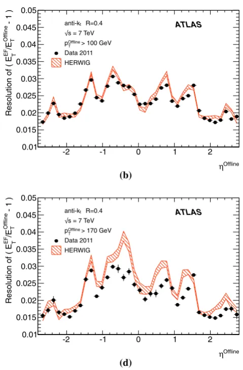
In Fig.8 the offset in transverse energy from the Event Filter, E_TEF, with respect to the offline jets is seen to vary over a range of approximately 10 % withη, with the offsets themselves being only two or three times larger than this range. Therefore the widths of the distributions of residu-als obtained when integrating over the entireηrange would result from a convolution of the true resolution and the vari-ation of the offset withη. The consequent resolution would appear artificially large, smeared by this additional factor of 10 %.

As a result, the mean offset and resolution in ET as a