Theses Thesis/Dissertation Collections
5-2017
Imaging Polarimetry with Polarization-Sensitive
Focal Plane Arrays
Dmitry V. Vorobiev
dxv2686@rit.edu
Follow this and additional works at:http://scholarworks.rit.edu/theses
This Dissertation is brought to you for free and open access by the Thesis/Dissertation Collections at RIT Scholar Works. It has been accepted for inclusion in Theses by an authorized administrator of RIT Scholar Works. For more information, please contactritscholarworks@rit.edu. Recommended Citation
polarization-sensitive focal plane arrays
By
Dmitry V. Vorobiev
A dissertation submitted
in partial fulfillment of the requirements for
the degree of Ph.D. in Astrophysical Sciences and Technology, in the School of Physics and Astronomy,
College of Science,
Rochester Institute of Technology
May 2017
Approved by
Prof. Andrew Robinson Date
ROCHESTER INSTITUTE OF TECHNOLOGY
ROCHESTER, NEW YORK
CERTIFICATE OF APPROVAL
Ph.D. DEGREE DISSERTATION
The Ph.D. Degree Dissertation of Dmitry V. Vorobiev has been examined and approved by the dissertation committee as satisfactory for the dissertation requirement for the Ph. D. degree
in Astrophysical Sciences and Technology.
Dr. Zoran Ninkov, Dissertation Advisor Date
Dr. Grover Swartzlander, Jr., Committee Chair Date
Dr. Michael G. Gartley Date
Dr. Dean C. Hines Date
Dr. David W. Messinger Date
Dr. Andrew Robinson Date
and roads, and even to abandon physics, if circumstances
require it. I would resolve to do so more easily, that I now
see it’s a stupid plan troubling oneself to acquire a small
bit of glory, that they’ll always quarrel with you about it...
Fie on contested glory!”
Augustin-Jean Fresnel
September 25, 1816
Two years later, Fresnel published
Abstract
Astrophysical Sciences and Technology
Doctor of Philosophy
Imaging polarimetry with polarization-sensitive focal plane arrays
by Dmitry Vorobiev
Polarization is an intrinsic property of light, like frequency or coherence. Humans have
long benefited from our ability to distinguish light of different frequency based on its
color. However, our eyes are not sensitive to the polarization of light. Devices to measure
polarization are relatively rare and expertise in polarimetry even more so. Polarization
sensors based on micropolarizer arrays appear to be the first devices capable of bringing
polarimetric capability to a wide range of applications. Whereas previous polarimeters
were built to perform very specific measurements, the same micropolarizer-based camera
can be used on a telescope, a microscope, or with a conventional camera lens.
In this work, I investigate the operating principles of micropolarizer arrays using high
resolution 3D simulations and describe several strategies to fabricate and characterize
micropolarizer-based imaging polarimeters. Furthermore, I show how to incorporate the
device characterization into a calibrated demodulation procedure to extract polarimetric
quantities from the raw pixel intensities. As part of this effort, I show how the measured
sensor properties, like pixel throughput and contrast ratio, can be used to construct
a software model to produce synthetic observations of various scenes. These synthetic
data are a powerful tool to study the many effects which can give rise to systematic
and/or random errors during the data analysis process. Finally, I present the polarimetry
performed on several astronomical sources using the RIT Polarization Imaging Camera
and compare my results to previous measurements made with conventional polarimeters.
Using the current calibration of the RIT Polarization Imaging Camera, I was able to
achieve a polarimetric accuracy of ∼0.3% in images of extended objects and unresolved
This work would not have been possible without the support and guidance of my advisor,
Zoran Ninkov. I am deeply grateful to him for the advice and encouragement that I’ve
received over the last five years. I also thank Mike Gartley, Dean Hines, Dave Messinger,
Andy Robinson, and Grover Swartzlander for serving on my dissertation committee.
Their input dramatically improved this dissertation.
I owe a special thanks to Ray West and Roger Ketcheson of Moxtek, Inc., who funded
much of this research and were champions of this work within their company. I am also
grateful to Neal Brock of 4D Technology for his insights and continued support of my
research. The data used in this dissertation were acquired using cameras built by Finger
Lakes Instrumentation and I would like to thank Gary McAnally for his help with my
(sometimes) unusual and (always) very last minute requests.
During the six years I spent at RIT, I benefited enormously from the efforts of numerous
faculty, staff, and students. Jan Maneti and Rob Kraynik from the College of Engineering
machined many parts for me and helped me avoid more than one fabrication-related crisis.
Bruce Smith allowed me to occupy a part of his clean room for over two years, where
the first RITPIC prototypes were built. Peter Bajorski helped me developed a deeper
understanding and appreciation of statistics, through his course, book, and very engaging
discussions. Al Raisanen has been a constant source of intriguing ideas and fabricated
several key components for me, often on the weekend.
The simulations presented in this dissertation were performed on the RIT Research
Com-puting cluster Ion. The architecture of Ion is uniquely suited for large computations that
are not embarrassingly parallel. Ion is a wonderful tool in the kit of RIT’s researchers.
Ion’s genesis is due to the efforts and vision of Gurcharan Khanna and its continued
existence is largely thanks to the work of Paul Mezzanini and his small, but dedicated,
crew.
While studying at RIT, I was fortunate to meet Judy Pipher, Dan Watson, Craig
Mc-Murtry, and Bill Forrest, from the astronomy department at the University of Rochester.
Their knowledge and support were instrumental in the development of my own ideas.
Institute of Optics, who is a wizard and a dedicated mentor.
The on-sky evaluation of our instrument was done on the 0.9 m telescope operated by Todd
Henry and the SMARTS consortium at the Cerro Tololo Inter-American Observatory.
Todd and the staff at CTIO worked hard to ensure the success of my observing run; I am
especially grateful to Hernan Tirado and Humberto Orrego.
For the last seven years, I had the pleasure and privilege of studying astronomy. I was
given this opportunity when John McGraw invited me to join his research group at the
University of New Mexico, despite my questionable academic transcript. I learned what
good work looks like from John and Pete Zimmer. Their passion, creativity, work ethic,
and good humor are a constant inspiration. I am forever grateful to them for their
Certificate of Approval i
Abstract iii
Acknowledgements iv
Contents vi
List of Figures x
List of Tables xxix
Abbreviations xxx
1 Introduction 1
2 Polarization of Light 5
2.1 A Mathematical Description . . . 7
3 Production of Polarized Light 12 3.1 Polarization Upon Reflection . . . 13
3.1.1 Reflection from Dielectric Surfaces . . . 14
3.1.2 Reflection from Metal Surfaces. . . 16
3.2 Polarization from Scattering . . . 19
3.2.1 Rayleigh Scattering . . . 19
3.2.2 Mie Scattering . . . 22
3.3 Polarization from Anisotropic Materials. . . 26
3.3.1 Diattenuation due to Aligned Asymmetric Particles . . . 26
3.4 Intrinsically Polarized Sources . . . 28
3.4.1 Synchrotron Radiation . . . 28
3.4.2 Lasers . . . 32
3.5 Polarizers . . . 33
3.5.1 Polarizing Prisms . . . 33
3.5.2 Polarizers Based On Diattenuation . . . 33
3.5.2.1 Absorptive Polarizers. . . 34
4 The Wire Grid Polarizer 35 4.1 Simulations of Wire Grid Polarizer Performance . . . 38
4.1.1 Simulation Methods . . . 39
4.1.2 2D Simulations - Setup and Convergence Testing . . . 40
4.1.2.1 Testing Numerical Convergence in 2D . . . 40
Summary . . . 43
4.1.3 2D Simulations - Effects of Wire Shape and Spacing . . . 45
4.1.3.1 Effects of Wire Width . . . 45
4.1.3.2 Effects of Wire Spacing . . . 48
4.1.3.3 Effects of Wire Height . . . 51
4.1.4 3D Simulations - Effects of Wire Shape and Spacing . . . 54
4.1.4.1 Testing Numerical Convergence in 3D . . . 54
4.1.4.2 Effects of Wire Width . . . 55
4.1.4.3 Effects of Wire Spacing . . . 57
4.1.4.4 Effects of Wire Height . . . 59
4.1.5 A Comparison of 2D and 3D Simulations . . . 60
4.1.6 Comparing Simulations to Experimental Results . . . 61
4.1.6.1 Common Sources of Disagreement . . . 63
4.1.7 Summary of Wire Grid Polarizer Simulations. . . 65
5 Micropolarizer Arrays 66 5.1 Simulations of Pixelated Wire Grid Polarizers . . . 67
5.1.1 Simulation Setup . . . 68
5.1.2 Convergence of Non-rectilinear Structures . . . 69
5.1.3 Performance of Pixelated Polarizers . . . 70
5.2 Performance of Micropolarizer Superpixels . . . 73
5.2.1 Simulation Results . . . 74
5.2.2 Analysis Of Diffraction-induced Cross-talk . . . 76
5.2.3 Summary of Pixelated Polarizer Simulations . . . 79
6 Measurement of Polarization 80 6.1 Polarimetry With a Single Polarizer . . . 80
6.2 Snapshot Polarimeters . . . 82
6.2.1 Division of Focal Plane Polarimetry . . . 83
6.3 The Dual-Beam Technique . . . 84
6.4 Polarization-Sensitive Detectors . . . 85
6.5 Polarimetry With Non-ideal Polarizers . . . 87
6.5.1 Using Linear Least Squares . . . 89
6.5.2 Distribution of the Stokes Parameters . . . 91
6.5.3 Bias of Polarization Estimators . . . 93
7 Fabrication of Micropolarizer Array-based Polarimeters 99
7.1 Fabrication of Polarization-Sensitive Sensors . . . 99
7.1.1 Fabrication at RIT - Passive Alignment . . . 101
7.1.2 Fabrication at RIT - Active Alignment . . . 108
7.1.3 Alignment Using A Carrier. . . 110
7.2 Fabrication at 4D Technologies . . . 111
8 Performance and Calibration 112 8.1 Characterization of Device Properties . . . 113
8.1.1 Modeling the System Response . . . 114
8.1.2 Pixel Throughput . . . 116
8.1.3 Relative Transmission -tk . . . 118
8.1.4 Polarizer Efficiency -k . . . 121
8.1.5 Pixel Orientation -φk . . . 123
8.2 Simulating the Polarimetric Performance . . . 125
8.2.1 Simulated Observations of Point Sources . . . 125
8.2.1.1 Step 1. Generation of the Point Spread Function . . . . 125
8.2.1.2 Step 2. Modulating the PSF . . . 127
8.2.2 Effects of Sampling . . . 128
8.2.2.1 Case 1. Constant Photometric SNR. . . 129
8.2.2.2 Case 2. Constant Peak Intensity . . . 131
8.2.2.3 Case 3. Constant Sampling, Varying Flux . . . 133
8.2.3 Correcting the Systematic Drift . . . 134
8.2.4 Summary . . . 139
8.2.5 Effects of Sub-Pixel Displacement . . . 139
8.2.6 Simulated Observations of Extended Objects . . . 143
9 Data Analysis Techniques 145 9.1 Polarimetric Errors in Various Polarimeters. . . 146
9.2 Polarimetry of Unresolved Sources. . . 147
9.2.1 Photometric Calibration . . . 147
9.2.2 Demodulation Using Aperture Photometry . . . 148
9.2.2.1 Pixel Non-Uniformity Correction With Flat Fields . . . 148
9.2.2.2 Measure the Flux . . . 150
9.2.2.3 Non-uniformity Correction Using the Full Characterization152 9.2.3 Polarimetry of Spatially Resolved Sources . . . 154
9.2.3.1 Demodulation Using a Per-Pixel Calibration . . . 154
10 Initial On-Sky Evaluation 158 10.1 Evaluation of the Gen 1 Prototype . . . 158
10.1.1 Data Processing . . . 159
10.1.2 Polarimetric Analysis . . . 160
10.2 Evaluation of the Gen 4 Prototype . . . 162
10.2.1 Polarimetry of Point Sources . . . 163
10.2.1.2 HD 78344 . . . 167
10.2.2 Polarimetry of Planets . . . 169
10.2.2.1 Jupiter . . . 169
10.2.2.2 Saturn . . . 179
10.2.2.3 Venus . . . 181
10.2.3 Observations of Nebulae . . . 184
10.2.3.1 Hen 401 . . . 185
10.2.3.2 Hen 404 . . . 187
10.2.3.3 Frosty Leo. . . 190
11 Conclusion 192 11.1 Design and Performance of MPA-based Sensors . . . 192
11.2 Polarimetry with MPA-based Sensors . . . 194
11.2.1 Device Nonuniformity and Characterization . . . 194
11.2.1.1 Performing the Characterization . . . 195
11.2.1.2 Determining the Quality of Device Characterization . . . 196
11.2.2 Developing an Observing Strategy . . . 197
11.2.3 Notes on Data Analysis . . . 198
11.3 Performance of RITPIC and Future Outlook . . . 198
11.3.1 Expected Performance of Similar Devices . . . 199
11.4 Promising Science Cases . . . 199
11.5 A General Purpose Polarimeter . . . 201
A Dissemination of Results 202
1.1 Left: A sketch by Lomonosov of a “fiery arc” surrounding Venus, caused by light refraction in the Venusian atmosphere. Right: a photo of the same phenomenon during the 2004 transit ©Lorenzo Comolli. Used with permission. . . 2
2.1 Left: Electromagnetic waves oscillate in a plane orthogonal to the direction of propagation. The frequency of oscillation is related to the energy of the photon and is often expressed in terms of the associated wavelength, λ. Right: The direction of oscillation in the plane of oscillation describes the polarization of a single photon. In this case, the photon is linearly polarized at 45◦ with respect to the x-axis. . . 6
2.2 The polarization of a single photon, or the average polarization of a col-lection of photons, can be described by the path that is traced by the electric field vector in the (ˆx - ˆy) plane perpendicular to the direction of motion of the photon(s). The polarization can be purely linear, circular (a combination of two orthogonal linear states out of phase by π
2) or elliptical. 6 2.3 The Poincar´e sphere can be used to specify the polarization state as a set of
coordinates on its surface. Furthermore, it is a useful way to demonstrate the relationship between the Stokes parameters and the polarization state. Notice that polarization states that are purely linear or purely circular reside along the equator and at the poles, respectively. The rest of the surface corresponds to more general, elliptical states. . . 10
3.1 Randomly polarized light can become strongly polarized when reflected off a surface, with the angle of polarization parallel to the surface of reflection (and perpendicular to the plane of incidence). . . 13
3.2 The reflection of light is highly dependent on the polarization of the in-cident radiation and the geometry of the reflection. The reflection coef-ficients for the amplitude of the electric field (given by Equations 3.1 & 3.2, ni = 1, nt= 1.50) depend highly on the angle of incidence. At Brew-ster’s angle,θB (dashed line), the amplitude coefficients and the reflection coefficients for electric field components parallel to the plane of incidence (perpendicular to the reflecting surface) reach zero and the reflected light is polarized parallel to the reflecting surface. . . 15
3.3 Left: The Stokes parameters I and Q describe how randomly polarized light can become highly polarized through a reflection from a dielectric ma-terial. At normal incidence,Q = 0 (the ˆx and ˆy components are reflected equally) and it increases with angle of incidence until Q=I at Brewster’s angle. In other words, at this point the intensity of light polarized parallel to the surface is equal to the total intensity and theDOLP = 1 (Right). 16
3.4 Left: Reflection coefficients for the electric field components perpendicular
and parallel to the plane on incidence, for 550 nm light reflecting off an aluminum mirror. The parallel component is suppressed at large angles of incidence, but never reaches 0, like for dielectrics. The reflection is minimal at the angle of principal incidence, indicated by the vertical dashed line. Right: The Stokes parameters show the changes in the reflection coefficients by a decrease in the total intensity, I, and an increase in Q. . 17
3.5 Left: The degree of polarization imparted to a randomly polarized beam
during a reflection from a metal. Right: Telescopes with fold mirrors exhibit large instrumental polarization. . . 18
3.6 Left: When randomly polarized light interacts with an atom or molecule
(orange circle in figure), the scattered photons will display a range of polar-ization states. The photons which are scattered in the plane orthogonal to the direction of propagation of the incident light will be completely linearly polarized. Right: Photons that are scattered at any other scattering angle will have a range of polarizations. Generally, the degree of polarization decreases as the scattering angle approaches α= 0◦ orα= 180◦. . . 20
3.7 Because the Sun’s rays are nearly parallel when they enter the Earth’s at-mosphere, there exist regions in the sky where many photons are scattered at an angle α ≈ 90◦, which creates very strong linear polarization along the line of sight toward those regions. This region of maximum polariza-tion depends on the posipolariza-tion of the Sun and it changes throughout the day and year. For example, at sunset and sunrise the sky near zenith is highly polarized. . . 21
3.8 Rayleigh scattering produces primarily linearly polarized light, with the DOLP as a strong function of the scattering angle (Left). The DOLP is maximal for scattering angles near α= 90◦, and minimal in the solar and anti-solar directions. In practice, multiple scattering in the atmosphere decreases the maximum observed DOLP to ∼ 0.8. The angle of linear polarization follows a circular pattern, centered on the Sun (Right). . . . 22
3.9 The radiation patterns for two orthogonal components of the electric field, for a wave scattered by a dieletric sphere with dimeter of 1µm can be very different. Here, the wave is incident from the left (180◦) and the amplitude is shown on a logarithmic scale to emphasize the difference between the two components. The patterns also strongly depend on the wavelength of light. These patterns were calculated using Scott Prahl’s convinient web-based Mie scattering calculator (http://omlc.org/calc/mie_calc.html). . . 25
3.11 Left: Elongated dust grains preferentially absorb the electric field compo-nent parallel to their “long” axis. If there is a mechanism that aligns the dust grains, they can polarize the light from background objects. Right:
Dust samples brought back to Earth from interplanetary space show strong evidence that these elongated dust grains exist throughout the Galaxy. . 26
3.12 Relativistic charged particles that are accelerated into circular orbits by magnetic fields emit synchrotron radiation. The polarization of this light depends strongly on the direction of radiation; for example, light emitted in the plane of the orbit is linearly polarized in that plane. . . 29
3.13 Relativistic charged particles that are accelerated into helical orbits by magnetic fields emit synchrotron radiation. The polarization of this light depends strongly on the direction of radiation; for example, light emitted in the plane of the instantaneous circular orbit is linearly polarized in that plane. . . 30
3.14 Left: The Crab Nebula is a large remnant of a supernova that was observed
in 1054 CE. This is a map of the flux in the visible V band. Right: The Crab Nebula shows a strong and complex polarization pattern (white cor-responds to large polarization), with peak fractional polarization of∼30%. Observations of D. Vorobiev, made using the SMARTS 0.9 m telescope at Cerro Tololo Inter-American Observatory. . . 31
3.15 Some lasers use Brewster windows, due to their extremely low reflectivity for the parallel polarization states. Only these states remain long enough to escape the resonator cavity and all modes of these lasers have the same polarization. . . 32
3.16 Some laser crystals are anisotropic and show higher gain for certain polar-ization states. . . 32
3.17 Many polarizing prisms have been invented by exploiting birefringent crys-tals and polarization upon reflection of dielectric materials. Most polariz-ing prisms produce highly polarized light, across a broad wavelength range. 34
4.1 Left: A wire grid polarizer is fabricated by aligning thin conducting wires,
which preferentially absorb the electric field components parallel to the wire orientation. The wire width and spacing needs to be smaller than the wavelength of light for the polarizer to efficient at blocking the unwanted polarization states. Right: In 1960, a wire grid polarizer for the near-infrared regime was fabricated by evoparting metal onto the ridges of a blazed diffraction grating. . . 36
4.3 Simulated broadband performance of a modern wire grid polarizers, made from aluminum (Al), gold (Au), and a perfect electrical conductor (PEC). These polarizers are very efficient at transmitting the polarization states perpendicular to the wire direction (Left), and blocking the state parallel the wire direction (Right). These curves (especially the transmission of the desired state) show that the polarizer reaches optimum performance when the wavelength of light becomes about 10× larger than the wire width, at
λ≈1µm. . . 37
4.4 Left: A conventional wire grid polarizer was simulated in 2D by modeling an aluminum wire with a rectangular cross-section on an SiO2 substrate. The light source originates inside the glass substrate∼2µm above the wire. The reflected and transmitted components are measured 3µm and 5µm above and below the polarizer, respectively. The simulation uses periodic boundary conditions (orange vertical lines) in the ±ˆxdirections, resulting in an infinitely repeating array of wires (Right). . . 41
4.5 We simulated structures using a wide range of mesh sizes, to determine when the structures were sufficiently resolved. We found that in 2D, sim-ulations began to numerically converge when the simulation mesh was smaller than 4 nm. . . 42
4.6 The size of the smallest mesh cell determines how well the simulation reproduces the desired geometry. This effect can be seen in refractive index map of the simulated structures. Plots along the bottom of the figure show the profile of the refractive index of each wire. . . 42
4.7 Left: Our 2D simulations began to numerically converge when the mesh
was smaller than 4 nm. Right Increasing the number of PML layers was effective at improving the estimation of the transmitted TE component (the state transmitted by the polarizer), but not of the TM component (the state reflected by the polarizer). . . 43
4.8 The numerical convergence of simulations can also be seen in the distribu-tion of the amplitude of the electric field. This figure shows the electric fields for a TE pulse (which is mostly transmitted by the polarizer). High resolution simulations are required to model very localized regions of high electric field intensity (though this may not represent fabricated structures, if they lack similar definition). . . 44
4.10 Electric field intensity cross-sections for 8 simulations of wires with increas-ing widths, for a TE pulse, which is mostly transmitted by the polarizer. Black rectangles correspond to the wire cross-section. These results are for light at a wavelength of 667 nm. The intensity is normalized by the source power and shown on a linear scale. The wire height is 200 nm and the spacing between the wires is equal to the wire width. . . 46
4.11 Left: Transmission of the TM component for a wire grid polarizer with wire widths of 50 nm, 60 nm, 70 nm, 80 nm, 90 nm, 100 nm, 125 nm, 150 nm, 175 nm and 200 nm, with duty cycle and wire height fixed at 50% and 200 nm, respectively. In general, wire grids with thinner wires transmit less light at all wavelengths. Right: Reflection of the TM state is not strongly affected by wire width; however, wires with thickness>∼100 nm exhibit resonant behavior at shorter wavelengths. . . 47
4.12 Electric field intensity cross-sections for 8 simulations of wires with in-creasing widths, for a TM pulse, which is mostly reflected by the polarizer. White rectangles are drawn to help outline the edges of the wires. These results are for light at a wavelength of 667 nm. The intensity is normalized by the source power and shown on a logarithmic scale. The wire height is 200 nm and the spacing between the wires is equal to the wire width. . . 47
4.13 Left: Transmission of the TE component for a wire grid polarizer with wire air gap width of 25 nm, 50 nm, 75 nm, 100 nm, 125 nm, 150 nm, 175 nm and 200 nm. In general, wire grids with larger air gaps exhibit higher transmis-sion at all wavelengths. Right: Reflection of the TE state decreases with increasing wire separation. Wires with air gap widths <50 nm (blue line) exhibit resonant behavior in the visible regime. . . 49
4.14 Electric field intensity cross-sections for 8 simulations of wires with in-creasing air gap widths, for a TE pulse, which is mostly transmitted by the polarizer. Black rectangles correspond to the wire cross-section. These results are for light at a wavelength of 667 nm. The intensity is normalized by the source power and shown on a linear scale. The wire height is 200 nm and the wire width is 75 nm. . . 49
4.15 Left: Transmission of the TM component for a wire grid polarizer with air gap widths of 25 nm, 50 nm, 75 nm, 100 nm, 125 nm, 150 nm, 175 nm and 200 nm. In general, wire grids with smaller air gaps exhibit lower transmission at all wavelengths. Simulations with a 25 nm gap predict extremely low transmission and a complex wavelength dependence, hinting at the emergence of numerical errors or more complex resonant behavior. Right: Reflection of the TM state increases with decreasing wire spacing, with the largest changes in the visible regime. . . 50
4.17 Left: Transmission of the TE component for a wire grid polarizer with wire heights of 25 nm, 50 nm, 75 nm, 100 nm, 125 nm, 150 nm, 175 nm, 200 nm, 250 nm, and 300 nm. In general, wire grids with taller wires exhibit lower transmission at all wavelengths; however, in the visible range two systematic patterns emerge, with a height of ∼100 nm separating these two regimes. Right: Reflection of the TE state has a complex dependence on wire height. . . 51
4.18 Electric field intensity cross-sections for 8 simulations of wires with increas-ing height, for a TE pulse, which is mostly transmitted by the polarizer. Black rectangles correspond to the wire cross-section. These results are for light at a wavelength of 667 nm. The intensity is normalized by the source power and shown on a linear scale. The wire width is 74 nm and the duty cycle 50%. . . 52
4.19 Left: Transmission of the TM component for a wire grid polarizer with wire heights of 25 nm, 50 nm, 75 nm, 100 nm, 125 nm, 150 nm, 175 nm, 200 nm, 250 nm and 300 nm. In general, wire grids with taller wires exhibit lower transmission at all wavelengths. Right: Reflection of the TE state has a complex dependence on wire height. . . 53
4.20 Electric field intensity cross-sections for 8 simulations of wires with in-creasing height, for a TM pulse, which is mostly reflected by the polarizer. White rectangles are drawn to help outline the edges of the wires. These results are for light at a wavelength of 667 nm. The intensity is normalized by the source power and shown on a logarithmic scale. The wire width is 74 nm and the duty cycle 50%.. . . 53
4.21 Right: We found that in 3D, simulations began to numerically converge when the simulation mesh was smaller than 4 nm. Left: We simulated structures and varied the number of layers in the absorbing PML boundary, to determine when the reflections from the PML were sufficiently supressed. A significant decrease in relative error can be achieved by using∼26 layers in the PML. . . 55
4.22 Left: Transmission of the TE component for a wire grid polarizer with wire widths of 50 nm, 60 nm, 70 nm, 80 nm, 90 nm, 100 nm, 125 nm, 150 nm, 175 nm and 200 nm, with duty cycle and wire height fixed at 50% and 200 nm, respectively. In general, wire grids with thinner wires exhibit higher transmission at all wavelengths. Wires with widths>100 nm (solid black line) exhibit resonant behavior in the visible regime. Right: Reflec-tion of the TE state increases with increasing wire width. . . 56
4.24 Left: Transmission of the TE component for a wire grid polarizer with wire air gap width of 25 nm, 50 nm, 75 nm, 100 nm, 125 nm, 150 nm, 175 nm and 200 nm. In general, wire grids with larger air gaps exhibit higher transmis-sion at all wavelengths. Right: Reflection of the TE state decreases with increasing wire separation. . . 58
4.25 Left: Transmission of the TM component for a wire grid polarizer with air gap widths of 25 nm, 50 nm, 75 nm, 100 nm, 125 nm, 150 nm, 175 nm and 200 nm. In general, wire grids with smaller air gaps exhibit lower transmission at all wavelengths. Simulations with a 25 nm gap predict extremely low transmission and a complex wavelength dependence, hinting at the emergence of numerical errors. Right: Reflection of the TM state increases with decreasing wire spacing, with the largest changes in the visible regime. . . 58
4.26 Left: Transmission of the TE component for a wire grid polarizer with wire heights of 25 nm, 50 nm, 75 nm, 100 nm, 125 nm, 150 nm, 175 nm, 200 nm, 225 nm, and 250 nm. In general, wire grids with taller wires exhibit lower transmission at all wavelengths; however, in the visible range two systematic patterns emerge, with a height of ∼100 nm separating these two regimes. Right: Reflection of the TE state has a complex dependence on wire height. . . 59
4.27 Left: Transmission of the TM component for a wire grid polarizer with wire heights of 25 nm, 50 nm, 75 nm, 100 nm, 125 nm, 150 nm, 175 nm, 200 nm, 225 nm and 250 nm. In general, wire grids with taller wires exhibit lower transmission at all wavelengths. Right: Reflection of the TM state reaches the maximum after a wire height of∼75 nm. . . 60
4.28 We compare the results of 2D and 3D simulations of a single wire and a 3D simulation of a 50 wire region. All simulations show very similar results, even though the simulated region is very different in each case. It appears that 2D simulations can be an accurate representation of certain 3D structures, if one can exploit some symmetries (such as the length dimension of a long, skinny wire). . . 61
4.29 An SEM micrograph of the cross-section of a wire grid polarizer. The aluminum wires are approximately 74 nm wide, with a 50% duty cycle and a height of ∼150 nm. It is clear from the micrographs that the fabricated polarizers do not have perfectly straight wires and their profiles are not strictly rectangular; furthermore, the height of the wires is not uniform . 62
4.31 The real (Left) and imaginary (Right) components of the refractive index of aluminum found in the literature. The commonly used values from the book by Palik (1998) and CRC Handbook of Chemistry (Shiles et al., 1980), differ from more recent measurements of aluminum thin films by Lehmuskero et al. (2007) and McPeak et al. (2015). . . 64
5.1 a). A micro grid polarizer array fabricated by Moxtek, Inc. b) A scanning electron micrograph (SEM) of a set of 4 micro polarizer pixels. Lighter re-gions correspong to the wires and the darker rere-gions are opaque aluminum. The wire orientations are, clockwise starting at top left: 0◦, 45◦, 90◦, and −45◦. c) An up-close image of a single micro polarizer. . . . . 67
5.2 left: A scanning electron micrograph of a pixelated polarizer. The grey regions represent aluminum and black gaps are air. Each polarizer is sur-rounded by an opaque aluminum border. The wires are∼8µm long. Mid-dle: The simulated pixelated polarizers were created by etching gaps in an aluminum layer to create wires of finite length. In this case, the wires had a length of 8µm and a height, width and air gap of 200 nm, 74 nm and 74 nm, respectively. The wires were surrounded by an opaque aluminum gap 0.5µm wide. Right: The pixelated polarizers are simulated using peri-odic boundary conditions in thexˆandyˆdirections, to create an effectively infinite array of identical polarizers. . . 68
5.3 Left: Pixels with diagonal wires are more difficult to mesh using a
rectilin-ear grid. Right: These simulations converge at a similar rate as simulations of rectilinear structures, but with a systematically higher relative error. . 69
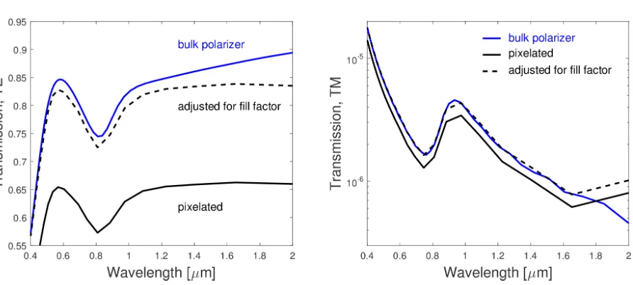
5.4 The transmission and reflection of the TE pulse for pixelated polarizers as compared to the conventional polarizer with similar wire parameters. The lower transmission of pixelated polarizers can be mostly explained by the non-uniform fill factor caused by the opaque border around each pixelated polarizer.. . . 70
5.5 The transmission of pixelated polarizers as compared to the conventional polarizer with similar wire parameters, for TE (Left) and TM (Right) com-ponents. The lower transmission for both states can be mostly explained by the non-uniform fill factor caused by the opaque border around each pixelated polarizer; however, even after scaling the transmission by a con-stant to adjust for the fill factor (dashed line), the pixelated polarizer does not show identical performance to conventional polarizers. . . 71
5.6 The transmission and reflection of the TM pulse for pixelated polarizers as compared to the conventional polarizer with similar wire parameters. . 72
5.7 Left: To model the performance of the whole MPA, pixels with different
5.8 Left: A top-down view of the simulated region, showing the 4 micropo-larizer pixels. Right: An isometric representation of the simulated region, showing the location of the electric field monitors. The glass substrate (which is on top of the blue micropolarizer layer) is not shown. . . 74
5.9 Left: The intensities recorded by monitors belonging to each pixel
orien-tation show mostly expected behavior. The pixel with 90◦ wires transmits most of the 0◦ polarized light, while the 45◦ and 135◦ pixels transmit roughly half of that value. Right: The contrast ratio in simulations with all 4 pixels can be calculated using a single polarized pulse. Here, we show the ratio of the intensities measured by the 0◦ and 90◦ pixels monitors in response to a 0◦ polarized pulse. . . 75
5.10 Left: The pixel with 135◦ wires transmits most of the 45◦ polarized light,
while the 0◦ and 90◦ pixels transmit roughly half of that value. Right:
The contrast ratio of the intensities measured by the 135◦ and 45◦ pixels monitors in response to a 45◦ polarized pulse. . . 75
5.11 Left: To measure the diffraction pattern due to a micropolarizer array, we
simulated an isolated micropolarizer surrounded by a large opaque border.
Right: The electric field was recorded by a normal-sized monitor and an
extended monitor, to show the diffracted light. . . 77
5.12 The electric field intensity (log scale) distribution for 400 nm (Left) and 2000 nm light (Right) transmitted by a 0◦ micropolarizer. The white dashed lines show the location of a 9µm×9µm region, 5µm below the micropolarizer. . . 77
5.13 Fraction of light measured by a central monitor directly below the microp-olarizer and an extended monitor, which also captures the diffracted light (see Figure 5.11). Ideally, all light that passes through a single micropo-larizer would remain in a region directly below that pomicropo-larizer. . . 78
5.14 Left: Vertical monitors along the boundaries between individual pixels can
be used to measure the crosstalk from diffraction directly. Right: The intensity of light passing through the vertical boundaries between the 45◦ polarizer and its neighbors accounts for most of the intensity measured by the 45◦ monitor. . . 78
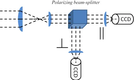
6.1 Division of time polarimetry. The degree and angle of linear polarization can be determined by measuring the intensity through a polarizer oriented along several directions. This is typically accomplished by rotating a sin-gle polarizer (blue arrow indicates the polarizer axis) or by using several polarizers in a filter wheel (as in done onThe Hubble Space Telescope). . 81
6.2 Division of intensity polarimetry. Polarimeters that sample the electric field along several orientations simultaneously can be built using beam-splitting optics and several detectors. The incident light is split and imaged in two or more channels simultaneously.. . . 82
6.3 Left: The Extreme Polarimeter (ExPo) uses beam splitters to record
6.4 Left: In some instruments, like RoboPol, the 4 separate images are recorded by a single detector, resulting in a very crowded image plane (Right). Adopted from Fig. 1 and Fig. 2 of King et al. (2014). . . 83
6.5 The dual beam modulation scheme uses a retarder and a beam splitter to capture two polarization states simultaneously, with a single or multiple detectors. The retarder is used to switch the orientation of both beams for each successive measurement. . . 84
6.6 Left: a color filter array divides the focal plane into sets of 2×2 “superpix-els” that determine the color of a section of a scene using the intensities measured by individual detector pixels. Right: A micropolarizer array-based polarimeter works in a fashion similar to a color sensor to measure polarization across a scene. Each polarizer pixel is matched spatially to a single detector pixel. Light passing through a polarizer pixel is modulated according to the polarizer’s orientation and the intensity is measured by the detector pixel.. . . 85
6.7 Optimal sampling on the Poincar´e sphere for linear (Left) and full Stokes (right) polarimetry. . . 88
6.8 The presence of Poisson noise results in a bi-variate distribution of the estimated Stokes parameter in the Q-U plane; here I show a set of 1000 synthetic measurements made with four ideal polarizers and non-ideal po-larizers that are not perfectly characterized. The miscalibrated non-ideal polarimeter introduces systematic errors into the estimation. . . 92
6.9 Synthetic observations of an unpolarized source show the positive bias of the p estimator. Whereas q and u are distributed around a mean of 0, hpi= 0.0021. The overestimation becomes worse as the scatter of q and u
increases. . . 93
6.10 Left: The distance from the origin to a point in the q-u plane is an
esti-mate of the fractional polarization p, while the angle made by this vector with respect to the q-axis is twice the estimated angle of linear polariza-tion. Right: The distribution of the magnitudes, p, is given by the Rice distribution, which can be used to calculate the probablity of measuring a valuepfor a source with intrinsic polarization p0. In the presence of noise, there is zero probability to measure a value p/σp = 0. . . 94
6.11 Left: The maximum likelihood estimator suggested by Simmons and
Stew-art (1985) is that value of p0 that is a solution to equation ∂p∂F0(p, p0) = 0 (eq. 6.8); there is a threshold value ofp= 1.41, below which the measured value of p is consistent with p0 = 0. Right: The estimator suggested by Wardle and Kronberg (1974) is the value p0 which solves equation 6.9. In this case, too, there is a threshold value ofp= 1, below which the measured polarization is consistent withp0 = 0. . . 95
6.12 Left: The variance for the q and u parameters can be used to estimate
7.1 Left: A wafer with several sensors ready to be diced and packaged (image: www-ccd.lbl.gov). Middle: A packaged CCD. The die has been cut from a wafer, attached to a ceramic carrier and wire-bonded to the metal pins of the carrier. Right: A microgrid polarizer on a thin glass substrate. . . 100
7.2 The imaging system used to determine MPA-CCD alignment is based on a compact microscope, CCD camera and a long working distance (LWD) mi-croscope objective. The LWD objective is required because the alignment procedure requires imaging of the CCD through the polarizer substrate, which is 0.7 mm thick. This is much larger than the working distance of conventional objectives.. . . 102
7.3 Left: A cross-section of the MPA-CCD pixels. From the top, down there
are 5 distinct regions: glass polarizer substrate, the thin polarizer layer, a gap (filled with air or epoxy), a layer of CCD microlenses that demarcate the pixels of the CCD, a layer of gate electronics and the bulk epitaxial layer with the depletion region. Right: An isometric view of the MPA-CCD system, showing exact alignment between the grid formed by MPA pixels and the grid formed by CCD pixels. . . 103
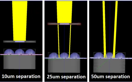
7.4 Because the polarizer is at the focal plane of the optical system, it is illuminated using converging light. As the separation between the polarizer and the sensor (in this case with microlenses) increases, the projected area of the polarizer pixels decreases. This figure shows a converging beam of polarized light. The middle polarizer blocks all of the light, while its neighbors transmit light. As the polarizer is moved away from the sensor, light from the left and right pixels ends up in the middle pixel. This is one example of optical crosstalk. Source: figure is courtesy of Kenneth Fourspring, personal communication. . . 104
7.5 Setup for alignment of MPA to CCD sensor. The CCD is held in a alu-minum chuck and is positioned inˆx−yˆ−θˆusing two linear stages stacked vertically on a rotation stage. The actuators of the stages are labeled in the figure. The z-distance between the polarizer and the CCD is controlled using another linear stage. The alignment of the MPA-CCD system is de-termined using a long working distance microscope objective and a CCD camera. The illumination source is fiber-coupled to the microscope system. 105
7.6 Close up of the assembly that holds the CCD and the micropolarizer array. 106
7.7 Left: An image acquired of the MPA at the physical edge of the MPA. The
jagged substrate and square pixels of the polarizer are clearly seen. A line is created to indicate the alignment of the MPA. Right: An image of the same region, focused on the CCD that is below the polarizer. The CCD pixels appear as sets of bright and faint rectangles. The CCD grid can now be aligned with the line that indicates the MPA alignment. In this image, the CCD is slightly misaligned with the MPA grid. . . 106
7.9 Left: The polarization sensitive focal planes were fabricated in a clean room at RIT. The micropolarizer arrays were aligned to a CCD sensor using a vacuum wand and computerized translation stages (Right:) A close-up of the illumination system. Alignment was monitored by illuminating the system with linearly polarized light and reading out the CCD. . . 108
7.10 Left: This alignment setup offered four degrees of motion - rotation in the
plane of the sensor andˆx−ˆy−ˆzmotion. Right: The micropolarizer array was held with a vacuum wand. This is a simple but problematic way to manipulate the micropolarizer.. . . 109
7.11 Left: The translation stages used to manipulate the micropolarizer array
and sensor were computer-controlled; however, the alignment process was not automated. Right: I built an interface to operate the camera, perform on-the-fly calibration, and provide real time feedback on the state of the alignment. . . 109
7.12 The 2nd generation prototype of a micropolarizer-based polarization sensor fabricated at RIT, using active alignment. . . 110
7.13 A carrier can be used to position the micropolarizer array above the sensor. This cross-section shows how a carrier can be used to avoid crushing the wire bonds that connect the CCD to the CCD carrier.. . . 110
7.14 The 3rd generation prototype of a micropolarizer-based polarization sensor fabricated at RIT, using active alignment. This design uses an aluminum carrier to hold the micropolarizer suspended above the sensor, with an air gap between them. . . 111
8.1 The polarization sensors were characterized using a rotating linear polarizer and an integrating sphere. The filter is placed before the sphere to avoid any polarization from a tilted glass plate. . . 113
8.2 The median response for pixels oriented along 0◦, 45◦, 90◦, and 135◦ to polarized light with a range of angles. The error bars show the standard deviation of pixels with the same orientation, at a particular angle. . . . 115
8.3 Full sensor area, uniformly illuminated by unpolarized light. The small, bright regions in the corners are uncovered areas of the sensor, which are used to calculate the throughput of the micropolarizer array (center). . . 117
8.4 Left: The camera head, with the front plate removed. The silver square
in the middle is the micropolarizer array, surrounded by the white ceramic carrier. Middle: To avoid the polarizing effects of the carrier, I used a mask to baffle the sensor. Right: the baffle covers more of the edges than necessary, however, the resulting active area (yellow square) is still a large fraction of the sensor. . . 118
8.5 Histograms of the mean-normalized transmissions, tk, for pixels of each orientation. The throughputs are systematically different for pixels with different orientations. There is a broad distribution of transmissions even for pixels of the same orientation. . . 119
8.7 Histograms of the polarizer efficiency, ek, for pixels of each orientation. The efficiency is similar for pixels with different orientations, with only the 135◦ pixels showing a systematic difference.. . . 121
8.8 Spatial distribution of polarizer efficiency, k for each pixel orientation, normalized by their own mean value. The spatial distribution of k and tk are only roughly similar (showing a top-down gradient) to the distribution of throughputs,tk. . . 122 8.9 Histograms of the polarizer orientations, φk, for pixels of each orientation. 123 8.10 Spatial distribution of polarizer orientation. The scale shows offsets from
the nominal orientation. . . 124
8.11 Left: The initial Gaussian PSFs are generated in high resolution to allow
precise shifts; presumably, this is what the electric field distribution looks like before it is sampled by the sensor. Right: The continuous image is sampled by the sensor, according to the magnification / plate scale of the imaging system. . . 126
8.12 Left: The total intensity PSFs are modulated by the micropolarizer array
based on the intrinsic properties of the source. Weakly polarized stars appear relatively unchanged. Right: Highly polarized stars show a strong modulation pattern. For example, this object is polarized with an angle of 0◦, so the 0◦ pixels appear brighter than the rest. . . 127
8.13 Synthetic stars generated to have 2, 4, and 8 superpixels across their full-width at half-maximum in the focal plane. Each star has the same total flux. . . 129
8.14 The estimation of q, for stars with intrinsic q = 0, 0.05, and 0.5, using an ideal and non-ideal polarimeter. The total flux was held constant as the FWHM was increased (Figure 8.13). In each case, the scatter of the measurement is reduced by increasing the FWHM to 3 superpixels, with neglibile gains seen with higher sampling. . . 130
8.15 The estimation of u, for stars with intrinsic u = 0, using an ideal and non-ideal polarimeter. The total flux was held constant as the FWHM was increased (Figure 8.13). In each case, the scatter of the measurement is reduced by increasing the FWHM to 3 superpixels, with neglibile gains seen with higher sampling. . . 130
8.16 Synthetic stars generated to have 2, 4, and 8 superpixels across their full-width at half-maximum in the focal plane. Each star has the same peak intensity, but the total flux increases as the PSF grows larger. . . 131
8.17 The estimation of q, for stars with intrinsic q = 0, 0.05, and 0.5, using an ideal and non-ideal polarimeter. The peak intesity at each sampling was help constant, allowing the total flux to increase (Figure 8.16). In each case, the scatter of the measurement is reduced by increasing the FWHM sampling to 5 superpixels, with neglibile gains seen with higher sampling. 132
8.19 Synthetic stars generated to have 4 superpixels across their full-width at half-maximum in the focal plane. Each star has a different peak intensity and, as a result, photometric SNR. Note that the high SNR images appear saturated because the scaling was chosen to ease comparison with the faint case. . . 133
8.20 Synthetic stars generated to have 4 superpixels across FWHM. The peak intensity of each star was increased to increase the shot-noise SNR. The scatter about the true value decreases significantly for stars with SNR&300.134
8.21 Synthetic stars generated to have 4 superpixels across their FWHM. The peak intensity of each star was increased to increase the shot-noise SNR. The scatter about the true value decreases significantly for stars with SNR
&750. . . 134
8.22 The estimation of q, for stars with intrinsic q = 0, 0.05, and 0.5, using an ideal and non-ideal polarimeter. The total flux was held constant as the FWHM was increased (Figure 8.13). . . 135
8.23 The estimation of u, for stars with intrinsic u= 0, using an ideal and non-ideal polarimeter. The total flux was held constant as the FWHM was increased (Figure 8.13). . . 136
8.24 The estimation of q, for stars with intrinsic q = 0, 0.05, and 0.5, using an ideal and non-ideal polarimeter. The peak intesity at each sampling was help constant, allowing the total flux to increase (Figure 8.16). In each case, the scatter of the measurement is reduced by increasing the FWHM sampling to 5 superpixels, with neglibile gains seen with higher sampling. 137
8.25 The estimation of u, for stars with intrinsic u = 0, and q = 0, 0.05, and 0.5, using an ideal and non-ideal polarimeter. The peak intesity at each sampling was help constant, allowing the total flux to increase (Figure 8.16). In each case, the scatter of the measurement is reduced by increasing the FWHM sampling to 5 superpixels, with neglibile gains seen with higher sampling. . . 137
8.26 The estimation of q, for stars with intrinsic q = 0, 0.05, and 0.5, using an ideal and non-ideal polarimeter. The sampling was held constant at FWHM = 4 superpixels, and the SNR was varied, by increasing the peak intensity. . . 138
8.27 The estimation ofu, for stars with intrinsicu= 0, andq= 0, 0.05, and 0.5, using an ideal and non-ideal polarimeter. The sampling was held constant at FWHM = 4 superpixels, and the SNR was varied, by increasing the peak intensity. . . 138
8.28 The Stokesq estimation depends systematically on the position of the PSF center. The ideal polarimeter shows a consistent error with a period of 2 pixels and amplitude of ∼0.2%; however, the non-ideal polarimeter shows an additional error, likely due to imperfect calibration. . . 140
8.30 The Stokesuestimation depends systematically on the position of the PSF center. The ideal polarimeter shows a consistent error with a period of 2 pixels and amplitude of ∼0.2%; however, the non-ideal polarimeter shows an additional error, likely due to imperfect calibration. . . 142
8.31 The non-ideal polarizer shows sysetmatic errors that appear to be location-dependent. This can result from the way the device calibration is per-formed during data analysis (see Chapter 9). . . 142
8.32 An example of a simulated object blurred by seeing effects. This plot show the raw intensity in counts. . . 143
8.33 Left: A synthetic modulated image showing the raw intensity for an object
has uniform polarization degree and angle. Right: Here, only the darker features show significant polarization, so the modulation pattern is only seen in these regions. . . 144
9.1 Left: A raw image of the unpolarized standard star HD 90156. Right: Once
the full image is divided into subframes with pixels of the same orientation, the flux can be measured using conventional aperture photometry. . . 148
9.2 A non-specular screen can be used to acquire unpolarized “dome flats”, as long as the screen is illuminated along the telescope’s axis. For example, lamps arranged symmetrically around the aperture of the telescope do a decent job. Note that the dome slit was only open to take this photograph.149
9.3 Left: An unpolarized flat field image of RITPIC, showing large scale and
small scale throughput nonuniformity on the order of ±5%; some dust is also visible. Right: A histogram of the relative pixel throughputs for each pixel orientation. Each pixel orientation has a systematically different throughput from the other orientations. For example, the 0◦ pixels have lower throughput than 45◦ pixels. . . 150
9.4 Left: A Stokes I image of synthetic star with 5 superpixels across the
FWHM; because this isn’t a raw image, each image pixel corresponds to a superpixel in the focal plane. Right: A schematic showing typical settings used for aperture photometry. The hashed region indicates the gap between the aperture around the star and the annulus used to estimate the sky background. . . 151
9.5 The mean-normalized properties of the 0◦ pixels, in a small region of the array; several percent deviations from the mean are common for tk and φk. 152 9.6 The estimation of Stokes q for stars with intrinsic polarizationq = 0, 0.05
and 0.5, made by ideal and non-ideal polarimeters, as a star is translated across the array.. . . 153
9.7 The estimation of Stokes u for stars with intrinsic polarizationu = 0 and
q = 0, 0.05, and 0.5 as a star is translated across the array. . . 153
9.9 The estimation of Stokes q and u parameters for the object in Figure 9.8, without proper calibration. The two smaller spots have intrinsic values q
= 0.01 andu = 0. . . 156
9.10 The estimation of Stokes q and u parameters for the object in Figure 9.8, with image registration but no flat field correction. . . 156
9.11 The estimation of Stokes q and u parameters for the object in Figure 9.8, with image registration and flat field correction. . . 157
9.12 The estimation of Stokes q and u parameters for the object in Figure 9.8, with image registration and flat field correction. . . 157
10.1 Left: A mean-normalized flat field image in the Bessel B filter, showing
the full focal plane of RITPIC. The bright orange areas correspond to the uncovered regions of the sensor, while the darker blue section corresponds to the area covered by the micropolarizer. Uneven distribution of the ad-hesive is easily seen near the top and bottom edge of the micropolarizer.
Right: Looking only at the polarization-sensitive region, we see how the
transmission varies. Features like dust and scratches on the polarizer sub-strate are also apparent. Note: The high-frequency vertical and horizontal lines are not real; the flats have high-frequency features which easily cause aliasing when displayed. . . 159
10.2 Left: A raw inverted intensity image of Jupiter and its two moons (Bessel
B filter). Jupiter’s disk shows the same aliasing effects seen in the flats, because the same structure is present in this not-yet flat-corrected image.
Right: a flat-corrected image of Jupiter. The bright bands across the face
of Jupiter appear red in this color map. . . 159
10.3 Polarization analysis of Jupiter data acquired with RITPIC. The polariza-tion of the poles of Jupiter is immediately obvious. The face of Jupiter shows little polarization. Because the images are under-sampled, the po-larimetric accuracy in these images is limited to±0.02. Therefore, we find the poles to be polarized at the 9%± 2% level. . . 161
10.4 Left: RITPIC was mounted at the Cassegrain focus of the SMARTS 0.9 m
telescope. The white spot in the upper left was used to acquire unpolarized dome flats. Right: RITPIC is a very compact imaging polarimeter. . . . 162
10.5 Left: The sampling in the RITPIC focal plane was 0.12” per pixel and
0.24” per superpixel. Right: HD 90156 was observed using 5 different locations on the array. The dashed circles are centered on the location of each star and the numbers indicate the frame numbers that correspond to each location. . . 163
10.6 Estimation of the normalized Stokes paramaters, q and u for each frame, using a flat field correction. The error bars on each measurement represent the photometric SNR. . . 164
10.8 Estimation of the Stokes q and u parameters for each frame, using a com-bination of a flat field correction, as well as the efficiency and orientation data obtained in the lab. . . 166
10.9 Polarimetry performed by RITPIC for the unpolarized star HD 90156 using the broadband response of the CCD. . . 166
10.10Normalized Stokes parameters q and u, measured by RITPIC for the po-larized star HD 78344 in the V band. The error bars represent the scatter in the estimation (as 1 standard deviation). . . 167
10.11Polarimetry performed by RITPIC for the polarized star HD 78344 in the V band. . . 168
10.12Raw images of Venus, Jupiter and Saturn acquired with Gen 4 RITPIC at the 36” telescope at CTIO.. . . 169
10.13The Stokes q and u maps made using a median of 20 images of Jupiter in the Bessel R filter. The maximum polarization measured is ∼ q = 0.08 and u=−0.07 in the instrumental reference frame. . . 170
10.14The Stokes q and u maps aligned with the scattering plane, to match observations of Schmid et al. (2011). The maximum polarization measured is∼ q = 0.08. . . 170
10.15The uncertainty maps for the normalized Stokes parameters q and u, esti-mated using the variance-convariance of the linear least squares estimator and formal error propagation. . . 171
10.16Left: The Stokes I “intensity” map of Jupiter in the Bessel R filter. Right:
The fractional polarization of Jupiter, estimated using the degree of linear polarization. The polarization at the poles is ∼8%, and it rapidly and smoothly decreases towards the equator. . . 173
10.17Left: Degree and angle of polarization shown with a vector plot. Right:
Angle of polarization across the face of Jupiter shown as a colormap. . . 174
10.18Left: Polarization at the poles and limbs of Jupiter, as a function of re-ciprocal wavelength, measured by Gehrels et al. (1969) in April 1960, with scattering angleα =−10.6◦. Note that the asymmetry between the North and South pole polarization is minimal at∼500 nm. Right: The same mea-surements repeated in November and December 1963, with scattering angle
α = 8.9◦ and α = 9.8◦, respectively. Note that the largest discrepancy is now at ∼500 nm. ©AAS. Reproduced with permission. . . 175
10.19The Stokes q and umaps made by Schmid et al. (2011) during the testing of the Zurich Imaging Polarimeter. The scale is set between 1% (white) and -1% (black). The lines in the Q/I image show the slit positions for spectropolarimetry performed with the EFOSC2 instrument on the ESO 3.6m telescope. Reprinted from Schmid et al. (2011), Copyright (2011), with permission from Elsevier. . . 176
10.21A comparison of the East-West profile of the intensity and normalized Stokes parameter q for observations made with RITPIC (blue line) and ZIMPOL (black line). The ZIMPOL intensity profile was scaled to have the same peak value as the RITPIC profile. . . 178
10.22Polarization of Saturn and its ring system in Stokesqand u. Although the overall polarization is low, some large scale features are clearly seen, such as the polarization of the rings, the northern and southern hemisphere and the south pole. . . 179
10.23Left: A Stokes I “intensity” map of Saturn in the Bessel R band. Right:
The fractional polarization of Saturn closely matches the Stokes q maps, because there is very little signal in u.. . . 180
10.24The angle of linear polarization shows a complex, large scale pattern across the rings and disk of Saturn. . . 180
10.25Polarization of Venus in Stokes q and u. The strongest polarization is seen in Stokes q, with a maximum near the poles and a minimum in the direction of the Sun. . . 181
10.26Left: A Stokes I “intensity” map of Venus in the Bessel R band. Right:
The fractional polarization of Venus, estimated using the degree of linear polarization. The polarization at the poles is ∼4% and ∼1% at the lower latitudes.. . . 181
10.27The polarization is oriented at ∼ −45◦ with respect to the East-West direction across the entire disk of Venus. . . 182
10.28Previous polarimetric observations of Venus and the models of Hansen and Hovenier (1974) for the Venereal atmosphere. The red circle shows the integrated polarization in Stokesq measured by RITPIC in the Bessel R band and the square shows the polarization at the equatorial point. This figure is adopted from Fig. 12 of Hansen and Hovenier (1974)©American Meteorological Society. Used with permission. . . 183
10.29Raw images of some planetary (and protoplanetary nebulae) acquired with Gen 4 RITPIC at the 36” telescope at CTIO. The scale is the same in all images.. . . 184
10.30Normalized Stokes parameters q and u calculated for Hen 401 using 5 300 second exposures in the R filter. . . 185
10.31The R band Stokes I image and the degree of linear polarization map for Hen 401. . . 185
10.32Left: HST imaging of Hen 401 from Ueta et al. (2007) showing the total (a) and polarized (b) flux. Right: Maps of the degree (c) and angle (d) of linear polarization. ©AAS. Reproduced with permission. . . 186
10.33Left: The DOLP and AOLP of Hen 401 overlaid on the intensity image.
Right: a detailed map of the angle of linear polarization shows good
agree-ment withHST polarimetry. . . 186
10.34Normalized Stokes parameters q and u calculated for Hen 404 using 9 300 second exposures, without any filters. . . 187
10.36Left: HST imaging of Hen 404 from Ueta et al. (2007) showing the total (a) and polarized (b) flux. Right: Maps of the degree (c) and angle (d) of linear polarization. ©AAS. Reproduced with permission. . . 188
10.37Left: The DOLP and AOLP of Hen 404 overlaid on the intensity image.
Right: a detailed map of the angle of linear polarization shows good
agree-ment withHST polarimetry. ©AAS. Reproduced with permission. . . . 189
10.38The Stokes qandupolarization for Frosty Leo. Peak polarization is∼40% and -45%, respectively. . . 190
10.39 . . . 190
10.40 . . . 191
11.1 Several mechanisms for cross-talk exist in micropolarized-based sensors that use off-the-shelf devices.. . . 193
10.1 Comparison of the polarimetric analysis of two standard stars performed by RITPIC to previous measurements (DOLP0), made by 1. Gil-Hutton and Benavidez (2003) and 2. Wiktorowicz et al. (2014). . . 168
AOLP Angle Of Linear Polarization
DOLP Degree Of Linear Polarization
FDTD Finite-Difference Time-Domain
MPA MicroPolarizerArray
PML Perfectly Matched Layer
RCWA RigorousCoupled-WaveAnalysis
SEM Scanning ElectronMicroscope
&
To John and Pete
Introduction
On June 6, 1761, telescopes at observatories across Europe were pointed at the Sun to
observe the transit of Venus across the solar disk. About two dozen scientists reported
seeing the disk of Venus surrounded by “arcs of fire” as it crossed the solar limb and the
appearance of “blisters” on the solar limb (which was otherwise quite sharp) as Venus
began its egress. Several observers correctly attributed these phenomena to refraction
through what must be Venus’s atmosphere, with the most rigorous observations (Figure
1.1) and analysis performed by Michael Vasil’evich Lomonosov (Shiltsev, 2014).
For the next 200 years, the nature of the Venusian atmosphere remained a mystery. Some
suggested that the thick clouds consist of water vapor and hide a surface overgrown by a
tropical jungle. Eventually, “progress at the Research Laboratory of the Eastman Kodak
Company in sensitizing photographic plates to the [near]-infrared allowed” Adams and
Dunham (1932) to obtain spectra that showed the first evidence for a large amount of
CO2 and very little H2O; however, as CO2 is transparent, the composition of the opaque
clouds remained undetermined.
Debate continued into the 1960s and 1970s, with a wide range of constituents suggested
for the cloud make-up, including, water ice, carbon dioxide ice, hydrated ferrous chloride,
formaldehyde, hydrocarbons, hydrocarbon-amide polymers, ammonium nitride, aqueous
Figure 1.1: Left: A sketch by Lomonosov of a “fiery arc” surrounding Venus, caused by light refraction in the Venusian atmosphere. Right: a photo of the same phenomenon
during the 2004 transit ©Lorenzo Comolli. Used with permission.
solutions of hydrochloric and sulfuric acid, mercury, and polywater1. Spectroscopic
fea-tures alone provided only ambiguous interpretations. For example, the feafea-tures attributed
to water ice could also be produced by gaseous CO2. As a last resort, some began to look
at the angular distribution of the light reflected by the Venusian clouds.
As Venus orbits the Sun, the reflected light arriving at the Earth samples a wide range
of scattering angles. In the early 1970s, James E. Hansen and J. W. Hovenier developed
radiative transfer models that accurately treat the effects of multiple scattering on
polar-ization (Hansen,1971;Hansen and Hovenier,1971). Finally,Hansen and Hovenier(1974)
used their models and the high quality polarimetric observations of Venus made by Lyot
(1929), Coffeen and Gehrels (1969), and Dollfus and Coffeen (1970), to conclude that
“the particle properties deduced from the polarization eliminate all but one of the cloud
compositions which have been proposed for Venus. A concentrated solution of sulfuric
acid (H2SO4-H2O) provides good agreement with the polarization data.”
The characterization of the Venusian atmosphere is a spectacular example of the utility
of polarimetry in the study of the microscopic properties of scattering particles. However,
the measurement of polarization can also be used to infer the macroscopic geometry of
objects. This use of polarimetry was demonstrated byAntonucci and Miller (1985), who
used spectropolarimetry of active galactic nuclei to show that Type 1 and Type 2 Seyfert
galaxies probably host similar nuclei, containing an accretion disk surrounded by a dusty
torus, but observed along different lines of sight. Polarimetry is also useful for
spatially-resolved objects as a means of deriving depth information in a scene. This was elegantly
shown by Kervella et al. (2014), who studied the polarization of light echoes reflected
from the dusty shells around RS Puppis to determine a geometric distance estimate to
this Cepheid variable. Measurements of polarization are responsible for discoveries in
nearly all areas of astronomy, from solar system science and the study of planets around
other stars, to the study of large scale structure of the universe.
On Earth, the applications of polarimetry are even more numerous. Measurements of
po-larization have been identified as a key tool in the study of the Earth’s own atmosphere
and its aerosol content. Polarization can be exploited in microscopy and minimally
inva-sive medical diagnostic imaging. In industrial settings, polarimetry can be used in
prod-uct inspection and quality assurance systems. The amount of surface detail captured by
infrared imaging systems can be significantly increased through the use of polarization.
Despite dozens of potential applications, the adoption of polarimetric techniques has been
slow, because our most advanced detectors are insensitive to polarization. To determine
the polarization of light, we are forced to use polarization-sensitive optics to modulate
the intensity of light. However, these polarimeters rarely advance beyond temperamental
prototypes built in research laboratories, and even the most polished systems cannot be
easily adapted to perform a similar measurement in a different setting or field.
The relatively new class of imaging polarimeters based on micropolarizer arrays shows
potential to be the first “general purpose” polarimeter, in sharp contrast to the highly
specialized and idiosyncratic polarimeters of the past. In this work, I attempt to
estab-lish the level of precision and accuracy that can be achieved with these devices when
imaging point sources and extended objects. To this end, I propose characterization and
calibration techniques and describe several methods of data analysis. I also investigate
In an attempt to make this work self-contained and consistent with existing
conven-tions, the first few chapters provide an overview of the principles of polarization and
polarimetry. A mathematical description of polarization and the Stokes formalism are
introduced in Chapter2. In Chapter 3I describe some common sources and mechanisms
that produce polarized light. The wire grid polarizer, which is the basic building block
of polarization-sensitive detectors, is introduced in Chapter 4. Using high resolution
numerical models I investigate the effects of wire shape and spacing on the polarizer’s
performance and explore the challenges associated with these simulations. In Chapter
5, I present high resolution 3D simulations of pixelated polarizers and micropolarizer
ar-rays. A brief overview of techniques and instruments used for polarimetric measurements
is given in Chapter 6. Efforts to fabricate polarimeters using micropolarizer arrays and
CCDs at RIT are detailed in Chapter 7. In Chapter 8 I describe the method used to
characterize sensors based on micropolarizer arrays and the software tools I developed to
produce synthetic observations, which are used to study various sources of polarimetric
errors. The data analysis process is described in Chapter 9. The results of the on-sky
evaluation of the RIT Polarization Imaging Camera are presented in Chapter10. Finally,
Polarization of Light
Electromagnetic radiation is characterized by four fundamental properties: polarization,
frequency, intensity and coherence (Figure 2.1). The term “polarization” can refer to
the configuration of the electric field of a single photon, or the average preference of a
collection of photons for a specific state. The electric field of each photon is configured
at the time of emission such that the momentum of the photon-plus-emitter system is
conserved. The polarization of a single photon is described by the direction of oscillation
of the electric field in the plane perpendicular to the direction of propagation (Figure
2.2). If this angle, ψ, is constant, the photon is linearly polarized and its polarization is
described by this angle of linear polarization (AOLP). If this angle changes (rotates) as
the photon propagates, the photon can be described as having circular (or more generally
elliptical) polarization. Without a mechanism that affects the emitters in some systematic
way, the state of the electric field of one photon is independent from another. This is
typical of systems that are well described by the Maxwell-Boltzmann distribution (e.g.,
black body radiators).
If a number of photons do not show a preference for a particular polarization state, we
call this light unpolarized (or ”randomly polarized”) and its degree of polarization, p
1. Because our eyes are not sensitive to polarization, unpolarized light feels “natural”.
However, in many situations the light we observe is polarized at some level. Some emission mechanisms (for example, many kinds of lasers) emit photons with a strong
preference for a particular polarization state. Synchrotron radiation, which is emitted by
Figure 2.1: Left: Electromagnetic waves oscillate in a plane orthogonal to the direc-tion of propagadirec-tion. The frequency of oscilladirec-tion is related to the energy of the photon and is often expressed in terms of the associated wavelength, λ. Right: The direction of oscillation in the plane of oscillation describes the polarization of a single photon. In
this case, the photon is linearly polarized at 45◦ with respect to the x-axis.
relativistic particles accelerated in magnetic fields, is highly polarized and the preferred
polarization state changes from linear to circular depending on the viewing geometry.
Even sources that are traditionally treated as black body radiators (people, cars, etc)
can emit polarized infrared radiation. Furthermore, there exist several processes that
are ef