Generalized Nonparametric Smoothing with Mixed Discrete and Continuous Data

and Continuous Data

.

White Rose Research Online URL for this paper:

http://eprints.whiterose.ac.uk/103402/

Version: Accepted Version

Article:

Li, Degui orcid.org/0000-0001-6802-308X, Simar, Leopold and Zelenyuk, Valentin (2016)

Generalized Nonparametric Smoothing with Mixed Discrete and Continuous Data.

Computational Statistics & Data Analysis. pp. 424-444. ISSN 0167-9473

https://doi.org/10.1016/j.csda.2014.06.003

[email protected] https://eprints.whiterose.ac.uk/ Reuse

This article is distributed under the terms of the Creative Commons Attribution-NonCommercial-NoDerivs (CC BY-NC-ND) licence. This licence only allows you to download this work and share it with others as long as you credit the authors, but you can’t change the article in any way or use it commercially. More

information and the full terms of the licence here: https://creativecommons.org/licenses/

Takedown

If you consider content in White Rose Research Online to be in breach of UK law, please notify us by

Computational Statistics and Data Analysis 00 (2014) 1–23

Statistics and

Data Analysis

Generalized nonparametric smoothing with mixed discrete and

continuous data

Degui Li

, L´eopold Simar

, Valentin Zelenyuk

a_{Department of Mathematics, University of York, The United Kingdom}

b_{Institut de Statistique, Biostatistique et Sciences Actuarielles, Universit´e Catholique de Louvain, Belgium} c_{School of Economics and Centre for Efficiency and Productivity Analysis, University of Queensland, Australia}

Abstract

The nonparametric smoothing technique with mixed discrete and continuous regressors is considered. It is generally admitted that it is better to smooth the discrete variables, which is similar to the smoothing technique for continuous regressors but using discrete kernels. However, such an approach might lead to a potential problem which is linked to the bandwidth selection for the continuous regressors due to the presence of the discrete regressors. Through the numerical study, it is found that in many cases, the performance of the resulting nonparametric regression estimates may deteriorate if the discrete variables are smoothed in the way previously addressed, and that a fully separate estimation without any smoothing of the discrete variables may provide significantly better results. As a solution, it is suggested a simple generalization of the nonparametric smoothing technique with both discrete and continuous data to address this problem and to provide estimates with more robust performance. The asymptotic theory for the new nonparametric smoothing method is developed and the finite sample behavior of the proposed generalized approach is studied through extensive Monte-Carlo experiments as well an empirical illustration.

Keywords: Discrete regressors, Nonparametric regression, Kernel smoothing, Cross-validation, Local linear smoothing

1. Introduction

Rapid advance of computing power and wide availability of large data sets encourage many researchers to sub-stantially increase their attention to various nonparametric methods for estimating nonlinear regression relationship. One of the most popular nonparametric methods appears to be the local polynomial least squares method, considered by Stone (1977), Cleveland (1979), Cleveland and Delvin (1988), Fan (1992, 1993), Fan and Gijbels (1992), Ruppert and Wand (1994) and popularized by Fan and Gijbels (1996). This method has received even greater appeal when it is substantially empowered by the seminal work of Racine and Li (2004), which suggests a neat way to deal with discrete regressors in the context of nonparametric regression. Racine and Li’s work has inspired many interesting ap-plications in a wide range of areas, for example, by Stengos and Zacharias (2006), Maasoumi et al. (2007), Parmeter et al. (2007), Eren and Henderson (2008), Walls (2009), Hartarska et al. (2010), Henderson (2010), to mention just a few. In these works where Racine and Li (2004)’s approach is used, researchers are able to obtain new insights with much more confidence, as their approach is free from imposing any parametric form on the regression relationship, while using both continuous and discrete regressors without splitting the sample into sub-samples for each value of

the discrete variables. In most of the empirical as well as theoretical studies and software codes using the Racine and Li (2004)’s approach that we are aware of, the way this approach is applied is in the “default” or simple form that we will describe below.

Indeed, it became somewhat common to smooth the discrete regressors in local polynomial least squares almost automatically, perceiving that one should obtain better results than if the nonparametric estimator is applied to each group separately (see Li and Racine, 2007; and the references therein). While this perception appears to hold in various cases and is supported by the simulations conducted by Racine and Li (2004) for the case of local constant fitting, in this article we illustrate that in some cases it may not be the case and smoothing the discrete variables can actually deteriorate substantially the resulting estimator of the regression function. In some situations, even, a fully separate estimation for each group identified by the discrete (or categorical) variable may give more accurate results (e.g., in terms of Mean Squared Error, MSE) than the approach with smoothing over the discrete variable. In these cases, the reduction in variance, or the efficiency gain due to smoothing of the discrete regressors, can be outweighed by a substantial bias introduced due to this smoothing. This may happen in both the small and relatively large samples, and so, for such cases, it may be preferable to make a fully separate estimation for each group.

We will see below that the source of the problem comes from the bandwidth structure suggested by the basic or default method appearing in the existing literature which we are aware of (see, for example, some references listed above). In this bandwidth selection procedure, a “simple” bandwidth scheme is proposed for the continuous variables, in the sense that the same bandwidth vector is taken across the various subgroups determined by the discrete variables, and then the bandwidths for the continuous and for the discrete variables are simultaneously determined. Hence, even if the resulting estimator of the bandwidth for a discrete variable takes the value of zero (i.e., no smoothing of this discrete variable with separate estimation by groups), the resulting bandwidths for the continuous variables are still restricted to be common to the various categories of the associated discrete variables. This may lead in some cases to “over-smoothing” in some groups and “under-smoothing” in the others.

To fix the ideas, suppose that we use the local constant kernel method (Nadaraya-Watson) and that we have two groups of observations (determined by one discrete variable) and only one continuous variable. Suppose in addition that in one group, the variable is relevant (the derivative of the regression function with respect to this variable is not zero), and in the other it is not relevant. In the latter group, the optimal bandwidth would converge to infinity as shown by Hall et al. (2007), whereas in the first group, it may converge to zero. A fully separate analysis which indicates “non-smoothing” on the discrete variable would capture this feature whereas the “simple-smoothing” would miss such a feature. The latter approach will provide a common bandwidth for the continuous variable that will under-smooth the regression in the group where the variable is irrelevant and over-smooth the regression in the group where it is relevant. This extreme case seems obvious but apparently it has been overlooked in the existing literature. We can also imagine less extreme situations where the phenomenon would be similar: small influence of the continuous variable in one group and a more complex structure in the other. When the local polynomial smoothing is used, the same problem would also appear if in one group the local polynomial approximation is not far from the true regression, but the structure in the other is globally much more complex. For example, for the local linear case, the optimal bandwidth would converge to infinity if the true regression is linear, or converge to zero if the true regression function is highly-nonlinear (Li and Racine, 2004). Obviously, the problem can even be more severe when estimating the derivative of the nonparametric regression function. We will briefly illustrate this point in one example below, showing the consequences which the simple-smoothing method could lead to. To the best of our knowledge, this phenomenon has never been analyzed in the literature using smoothing techniques for discrete variables. It is one of our objectives to investigate the consequence of such issue.

In this paper, we introduce a simple way to generalize and improve the commonly used smoothing methods and overcome the potential difficulties mentioned above. Specifically, in the bandwidth selection procedure, we allow different bandwidth parameters for the continuous variables in different categories of the discrete variables. We call this method the “complete-smoothing” approach in contrast to the simple-smoothing approach used in most of the existing literature and to the non-smoothing approach where the groups are treated fully separately. This smoothing approach is, of course, at a cost of somewhat higher computational complexity, but we will see later that the gain in precision of the regression estimate can be substantial. We will limit the presentation to the case of categorical discrete variables where each value of the discrete variables determines a group.

More generally and beyond the extreme cases described above, whether the bias beats the variance or not essen-tially depends on the degree of difference of curvatures of the regression relationship pertinent to each group identified

by the discrete variable and to some extent also depends on other aspects of the Data Generating Process (DGP) such as the size of the noise. Thus, in general,a prioriit is not clear whether it is better to smooth the discrete variables or to do a fully separate estimation (unless the latter is hardly reliable or impossible due to very small data in a given group) and, so far, there appears to be no formal rule of thumb for deciding on this dilemma. The complete-smoothing approach, that we suggest below, not only allows for smoothing the discrete variables, but also uses different band-widths for each group for the continuous variables. Since this encompasses both the non-smoothing approach and the simple-smoothing technique as special cases, we can expect more robust performance of the complete-smoothing approach, which will be investigated later in the paper.

One of the main messages of our paper is that when using the simple-smoothing approach, an additional as-sumption on “similar degree of smoothness” with respect to continuous variables is implicitly imposed for different categories of the discrete variables, and one should recognize or acknowledge it explicitly. Moreover, we show that such an additional assumption can distort the estimates substantially. While many examples can be used to illustrate the problem, we will deliberately take simple examples (a univariate continuous and univariate discrete variable to avoid the potential curse of dimensionality problem), to vividly illustrate the point. We will also suggest a way to overcome this problem, whenever it is numerically doable, and point out the numerical difficulties involved there as well as open questions that still remain.

The rest of this paper is organized as follows. Section 2 recalls the basic methodologies of the local linear least-squares method; Section 3 introduces the local linear complete-smoothing method and establishes the asymptotic theory; Section 4 illustrates how severe the problem can be through some extensive Monte-Carlo experiments and how the proposed complete-smoothing approach outperforms the simple-smoothing approach; Section 5 illustrates the issue with a real data set and Section 6 concludes and summarizes our main findings. Some technical assumptions and proofs of the theoretical results are given in Appendix A–C.

2. Local linear simple-smoothing

The point we aim to stress in this paper is a general phenomenon linked to nonparametric kernel-based regression, but we illustrate it through a method that appears to be the most popular in practice: the local linear least squares (LLLS) which is a particular case of local polynomial least squares (LPLS). Our remarks and suggestions could ob-viously be applied to other nonparametric kernel-based estimation methods such as the local non-linear least squares, and local linear quasi-likelihood methods (see, for example, Gozalo and Linton, 2000; Fr¨olich, 2006; Park et al., 2010). We summarize here the basic idea of the LLLS method, and can refer to Fan and Gijbels (1996), Pagan and Ullah (1999), and Li and Racine (2007) for details. This method allows flexible form through approximating locally the true unknown regression. Assume that the dependent variablesYi∈R,i=1, . . . ,n, are generated by the following

regression model:

Yi=m(Zi)+εi, (1)

whereZi = (Zic,Z d

i) withZ c

i ∈ R

p _{being continuous andZ}d

i being aq-dimensional discrete vector. We next focus

on the presentation for categorical unordered variables, but the same could be done for naturally ordered variables with slight modifications, see Racine and Li (2004) for details. In addition, we make the standard assumptions on the errors,εi, that they are independent random variables with

E(εi|Zi)=0 and Var(εi|Zi)<∞ a.s.,

although the methodology we will discuss may also apply to more sophisticated setups. The flexibility of the model is related to the fact that the unknown regression functionm(_·) is not specified. No particular parametric assumptions are made onm(_·) itself except for some smoothness properties onm(_·,zd_{). For the sake of simplicity, we assume}

thatm(_·,zd) is twice continuously differentiable with respect to its first pcontinuous arguments. Finally, we need also some regularity condition on the smoothness of the conditional density f(zc_|zd) with respect to thepcontinuous arguments.

mentioned above, we will limit our presentation to the case of local linear approximation (r=1). Extension to higher orders follows the same ideas but at a cost of more notational complexity. Consider the following local approximation:

m(u,v)≈αzc_,zd+βτ_zc_,zd(u−z c

), (2)

whereαzc_,zd ∈ R andβ_zc_,zd ∈ Rp are quantities to be estimated that, in general, vary with (zc,zd). To take only

neighboring observations around (zc_,zd_{), or to give more weights to them, when evaluating the least-squares criterion,}

the kernel approach is used. For the continuous variables we use a product kernel (but other multivariate kernels may also work), i.e.,

Kh(Zic−z c

)=

p Y

j=1

1

hj

Kj

Z_{i j}c ₋zc_j hj

!

, (3)

whereh =(h1, . . . ,hp) is a vector of bandwidths,Kj(·) is a standard univariate kernel function such as the univariate

standard Gaussian density,zc jis the j

th_{component ofz}c_andZc i =(Z

c i1,· · ·,Z

c ip)

τ_{. For the discrete vectors, we use the}

discrete kernel introduced by Racine and Li (2004), i.e.,

Λλ(Zid,z d

)=

q Y

ℓ=1

λI(Z d

iℓ,z

d ℓ)

ℓ , (4)

whereI(A) is the indicator function, withI(A) = 1 ifAholds, and 0 otherwise,λℓ _∈ [0,1] are bandwidths for the discrete variablesℓ=1, . . . ,q, andZd

i =(Z d i1,· · ·,Z

d iq)

τ_{. The LLLS or weighted least squares criterion at a given point}

(zc_,zd_{) measuring the quality of the approximation is thus given by}

Cn(αzc_,zd, β_zc_,zd;zc,zd)= n X

i=1

Yi−αzc_,zd−βτ_zc_,zd(Z c i −z

c

)

2

Kh(Zic−z c

)Λλ(Zid,z d

). (5)

We note that if for a particularℓ, we haveλℓ =0 (with the convention that 00 =1), then there is no smoothing of thisℓthdiscrete variable; i.e., the evaluation in (5) is done separately for each subsample determined by this discrete variable, with a commonh. At the other limit, if λℓ = 1, we do not take into account the discrete variableZ_id_ℓ in the analysis, i.e., all the sample points have weight in (5) which is independent from the value ofZ_id_ℓ. Letbαzc_,zd and bβzc_,zd minimize the criterionCn(·,·;z) withz=(zc,zd), then the proposed estimated value of the regression function

at the point (zc,zd), denoted bybm(zc,zd), is given bybαzc_,zd whereasbβ_zc_,zdgives the estimated value of the first partial

derivative ofm(·) with respect to the continuous variableszcevaluated at (zc,zd). As a common bandwidth is used to smooth over the continuous variables for different subgroups, we call such a method local linear simple-smoothing.

The bandwidth selection is a very important issue in nonparametric kernel-based estimation. The selection of appropriate bandwidths (h, λ) in (5) can be done by the cross-validation (CV) method, although many other approaches can be adopted such as the corrected AIC method. When adopting the CV approach, the values ˆhand ˆλare chosen to minimize

CV(h, λ)=

n X

i=1

h

Yi−bm(−i)(Zci,Z d ih, λ)

i2

M(Z_ic,Zd_i), (6)

where M(Z_ic,Zd_i) is a weight function trimming out boundary observations andbm(₋i)(Z_ic,Z_id|h, λ) is the

leave-one-out kernel estimator of m(Z_ic,Zd_i) with bandwidthsh and λ, i.e., estimated by minimizing (5), but leaving theith

observation out of the sample. The properties of the resulting estimatorbm(zc,zd) by using the CV bandwidth selection method have been described in the seminal paper by Racine and Li (2004) for the local constant case (r =0), and in Li and Racine (2004) for the local linear case. It is important to notice that, as is common in the nonparametric smoothing approaches, these results assume thathj → 0 for all j =1, . . . ,p, andnh1. . .hp → ∞asn → ∞. The

argument generally admitted in the existing literature is that it is better to smooth the discrete variable in (5), because the separate analysis on each separate subsample defined by the categorial variablesZd _{would correspond to the}

particular case when allλℓ =0,ℓ=1, . . . ,q. However, we indicate in the next section that it might not be the case in

some situations.

3. Local linear complete-smoothing

To simplify the argument, let us suppose that we have a univariate discrete variable defining two groups of obser-vations (the argument would be the same when considering all the subgroups defined by the multivariate categorical vectorZd). The DGP in the two groups may have different characteristics (shape of the regression function, curva-ture, or size of the noise). Extreme cases of such differences have been briefly described in the introductory section. Unless the sample size within one of the groups is very small, the CV bandwidth selection procedure described above would provide a small value of the tuning parameterλfor a relevant discrete regressor, resulting in the frequency method in the limiting case whereλ =0, and a commonh for different groups. Furthermore, we suppose that the continuous variableZc_{is also univariate. Extension to the case of multivariate continuous and discrete variables is}

straightforward. However, such extension may not be so useful because of the curse of dimensionality problem. As pointed out above for the extreme cases, the simple-smoothing based CV method might be inappropriate in many situations where some important characteristics of the DGP are quite different between the two subgroups. In such instances, having a common bandwidthhfor different groups may lead to under-smoothing (over continuous variables) for one group while over-smoothing for the other. While this may not matter asymptotically as long as the common bandwidth has the proper order, it happens to matter in the finite sample case (small and even relatively large ones), sometimes substantially, as illustrated in our examples in the next section. To address this issue, it might be better to do fully separate estimation within each subgroup, allowing the bandwidth over continuous variable to vary across different groups without smoothing for the discrete variable. Although, as pointed out by Li and Racine (2004), this may increase the variance, the bias could be lowered substantially, which would lead to the estimation with smaller MSE than the simple-smoothing method. We will show in the next section, through the Monte-Carlo simulations, that the loss in accuracy of the default simple-smoothing estimation method may be dramatic. However, it is well-known that if the sample size in one group is too small, one cannot hope to get sensible results with the separate local linear estimation. We next give a solution to address this problem.

A natural way is to allow different bandwidths for the continuous variable in the different subgroups which address the problem of over- or under-smoothing in subgroups, and allow smoothing over the discrete variable, as in Racine and Li (2004), to circumvent the problem that the number of observations in one subgroup might be too small. We call such method the complete-smoothing method. Formally, in the case of two subgroups defined by one discrete variable, the equation (5) defining the estimator could be replaced by

Cn(αzc_,zd, β_zc_,zd;zc,zd)= n X

i=1

Yi−αzc_,zd−βτ_zc_,zd(Z c i −z

c

)

2 Λλ(Zid,z

d

)

×

Kh(1)(Zic−z c

)InZ_id=zd(1)o+Kh(2)(Zic−z c

)InZ_id =zd(2)o, (7) wherezd_{(k),k =1,2, are the two possible values ofz}d_{. For simplicity, we use the same kernel function in the two}

subgroups, but allow potentially different bandwidthsh(1) andh(2) for these subgroups. Letem(zc_,zd_{) be the local}

linear estimated value ofm(zc_,zd_{) with complete-smoothing which minimizesC}

n(αzc_,zd, β_zc_,zd;zc,zd) with respect to αzc_,zd andβ_zc_,zd. It is clear that the general formulation we propose in (7) encompasses both the fully separate analysis

by groups (λ=0), and the simple-smoothing approach (h(1)=h(2)). Letµj=

R

ujK(u)duandνj= R

ujK2(u)du. Defineσ2m(zc,zd)=

ν0σ2(zc,zd)

f(zc_|zd_)P(Zd_=zd₎ and

bm,1(zc) =

1 2µ2m

′′_(zc_,zd

(1))h2(1)+λ(1−p1)f(z c

|zd₍₂₎₎

p1f(zc|zd(1))

h

m(zc,zd(2))₋m(zc,zd(1))i,

bm,2(zc) =

1 2µ2m

′′_(zc_,zd

(2))h2(2)+λ p1f(z c

|zd₍₁₎₎

(1−p1)f(zc|zd(2))

h

m(zc,zd(1))₋m(zc,zd(2))i,

whereσ2₍

·,_·) and f(_·|·) are defined in Assumption 3 in Appendix A and 0 <p1 =P(Zd =zd(1)) <1. We next give

the asymptotic distribution theory for the local linear complete-smoothing estimatorem(zc_,zd_).

Theorem 3.1. Suppose that Assumptions 1–4 in Appendix A are satisfied. If zd_=zd_{(1), we have}

p

nh(1)

e

m(zc,zd(1))−m(zc,zd(1))−bm,1(zc)

_d

If zd _=zd_{(2), we have} p

nh(2)

e

m(zc,zd(2))₋m(zc,zd(2))₋bm,2(zc)

_d

−→Nh0, σ2m(z c

,zd(2))i. (9)

We next derive the optimal bandwidths for the local linear complete-smoothing estimator. Letme(−i)(Zci,Z d

i|h(1),h(2), λ)

be the leave-one-out local linear complete-smoothing estimated value ofm(Zc i,Z

d

i) with tuning parametersh(1),h(2)

andλ. Then, similarly to the CV method introduced in Section 2, we define

CV(h(1),h(2), λ)=

n X

i=1

h

Yi−me(₋i)(Zic,Z d

ih(1),h(2), λ) i2

M(Z_ic,Z_id). (10)

The optimal bandwidths [ˆh(1),hˆ(2),λˆ] are the values which minimize CV(h(1),h(2), λ). Define

ψ1(h(1), λ) = p1

Z

b_∗(zc,zd(1))h2(1)+

λ(1₋p1)f(zc|zd(2))

h

m(zc_,zd₍₂₎₎

−m(zc_,zd₍₁₎₎i

p1f(zc|zd(1))

2

×M(zc,zd(1))f(zc_|zd(1))dzc, ψ2(h(2), λ) = (1−p1)

Z

b_∗(zc,zd(2))h2(2)+

λp1f(zc|zd(1))

h

m(zc_,zd₍₁₎₎

−m(zc_,zd₍₂₎₎i

(1₋p1)f(zc|zd(2))

2

×M(zc,zd(2))f(zc_|zd(2))dzc,

whereb_∗(zc,zd)=₂1µ2m′′(zc,zd). Define

χ(h(1)) = ν0

h(1)

Z

σ2(zc,zd(1))M(zc,zd(1))dzc, χ(h(2)) = ν0

h(2)

Z

σ2(zc,zd(2))M(zc,zd(2))dzc.

We next give the asymptotic expansion of CV(h(1),h(2), λ), which is critical to derive the asymptotic property of the optimal bandwidths [ˆh(1),hˆ(2),λˆ].

Theorem 3.2. Suppose that the conditions in Theorem 3.1 and Assumption4′_{are satisfied. Then, we have}

CV(h(1),h(2), λ)=CV1+ Φ(h(1),h(2), λ)+s.o., (11)

whereCV1:=Pni=1ε 2

iM(Z c i,Z

d

i)is independent of the tuning parameters,

Φ(h(1),h(2), λ)=nhψ1(h(1), λ)+ψ2(h(2), λ)

i

+χ(h(1))+χ(h(2)),

and s.o.represents some terms with smaller asymptotic order.

Define

MSE(h(1),h(2), λ)=

n X

i=1

h

m(Z_ic,Zd_i)₋em(₋i)(Zic,Z d

ih(1),h(2), λ) i2

M(Zc_i,Z_id). (12) In the proof of Theorem 3.2 in Appendix B, we show that

MSE(h(1),h(2), λ)= Φ(h(1),h(2), λ)+s.o. (13) Letting [h_∗(1),h_∗(2), λ_∗] be the minimizer to MSE(h(1),h(2), λ), by Theorem 3.2 and standard argument such as the proofs of Theorems 3.1 and 3.2 in Li and Racine (2004), we have the following corollary.

Corollary 3.1. Suppose that the conditions in Theorem 3.2 are satisfied. Then, we have

ˆ

h(1)₋h_∗(1)

h_∗(1) =oP(1), ˆ

h(2)₋h_∗(2)

h_∗(2) =oP(1), ˆ

λ₋λ_∗

λ_∗ =oP(1). (14)

Furthermore, the asymptotic normal distributions in (8) and (9) still hold when[h(1),h(2), λ]are replaced by[ˆh(1),hˆ(2),λˆ].

We next compare the measurements of the MSEs between the local linear complete-smoothing and the local linear simple-smoothing. Let

MSE(h, λ)=

n X

i=1

h

m(Z_ic,Zd_i)₋bm(₋i)(Zic,Z d ih, λ)

i2

M(Z_ic,Z_id). (15) and [h0, λ0] be the minimizer to MSE(h, λ). Analogously, we can also show that

ˆ

h₋h0

h0

=oP(1),

ˆ

λ₋λ0

λ0

=oP(1). (16)

Noting that

MSE(h(1),h(2), λ)=MSE(h, λ)+s.o.

for the case ofh(1)=h(2)=handλ=o(h2_{), we may show that}

min

h(1),h(2),λMSE(h(1),h(2), λ)≤minh,λ MSE(h, λ). (17)

Using (14), (16) and (17), we can easily prove the following corollary, which indicates that in the large sample case, the MSE by using the optimal bandwidths chosen by our method is smaller than that by using the default optimal bandwidths.

Corollary 3.2. Suppose that the conditions in Theorem 3.2 are satisfied. Then, we have

MSE(ˆh(1),hˆ(2),λˆ)_≤MSE(ˆh,λˆ)

in probability.

In the next section, we will investigate the finite sample properties of the different approaches. This will fur-ther confirm the expected theoretical performance of our complete-smoothing approach over the simple-smoothing approach. In particular, we will find that the gain in precision may be substantial in practice.

4. Simulation studies

In this section, we present two simple examples that allow us to vividly illustrate the issue raised in the previous sections. We provide some “typical” pictures resulting from these simulated samples generated according to the scenario described below. We may not conclude general statements with one simulated sample, but the idea is to provide visualization of the problem. Throughout the simulation, we considered the following regression relationship

Yi=a1+a2Zid+b1Zic+b2ZidZ c

i +b3(Zic)

2_+b

4Zidsin(πZ c

i)+εi, i=1,· · ·,n. (18)

Varying the choice of the parameters in model (18) would lead to various examples explored in this section.

Example 4.1. (linear versus periodic regression)

Leta1 = 1,a2 = −1,b1 = 1,b2 = 0.1,b3 = 0,b4 = 2, withεi ∼ N(0, σε,i), whereσε,i = 2−Zd_i. Here, for

each simulation,Zc

i ∼U(−2,2) for the continuous variableZ

c_{and the discrete variableZ}d _{was set randomly at 1 if}

W >0.25 and set at 0 ifW _≤0.25, whereW _∼U(0,1). So, we randomly obtained about 75% of observations for group 1 (withZd

In this example, for group 2 (zd _{=0) we have a linear model with more noisy data and smaller sample size, and}

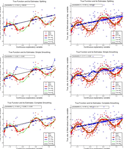
for group 1 (zd _{=1) we have a linear model (with different intercept and slope) plus a cyclical component. In Figure}

1, we present typical results of the estimation by using the three approaches: the fully separate estimation of the two subsamples (i.e., non-smoothing over the discrete variable, Approach 1), the simple-smoothing (i.e., smoothing the discrete variable with common bandwidth for the continuous regressor, Approach 2), and the complete-smoothing (i.e., smoothing the discrete variable and keeping potentially different bandwidths for the continuous variable, Ap-proach 3). Only two cases of sample size are provided in Figure 1:n =100 andn=400 (similar pictures have been obtained for other sizes).

From the left panels (n=100), we can see that the simple-smoothing (Approach 2) suffers from a serious drawback in this scenario and that the non-smoothing estimation (Approach 1) gives much better results both for n = 100 andn = 400. The complete-smoothing of Approach 3, encompassing the two preceding ones, does as well as the fully separate analysis for these samples. The fully separate estimation substantially outperforms the estimation with simple-smoothing over the discrete regressor, as the latter approach under-smoothes for group 2 and slightly over-smoothes for group 1. Note that for this example, the under-smoothing is more pronounced because group 1 dominates in the pooled sample by its larger size and so the common bandwidth selected in the CV optimization for (h, λ) is relatively close to what is optimal for group 1 in the separate estimation, while for the group 2, the true optimal bandwidth must in fact go to infinity to attain the correctly specified parametric model. The complete-smoothing (Approach 3) avoids such problem by allowing different bandwidths for the continuous regressorZc_{in the}

two groups.

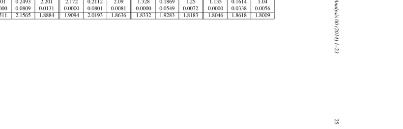
The numerical results of the Monte-Carlo experiment summarized in Table 1 further confirm the above analysis from Figure 1. Withn = 50,100,200,400, we conducted 500 Monte-Carlo replications for each case. The table provides the mean of the Approximate Mean Squared Error (AMSE) for each sample, averaged over 500 Monte-Carlo replications, i.e., AMSE = (1/M)PMg=1AMSEg, where the AMSE for each replicationg(g =1, . . . ,M with

M=500) is defined as

AMSEg=

1

n

n X

i=1

h

m(Zc_i,g,Zd_i,g)₋mb(Z_ic_,g,Z_id_,g)i2,

wherebm(·,_·) is the estimate of the true regression functionm(·,_·) by using the above three approaches, respectively. Table 1 also gives the estimated standard deviation of AMSE defined as

stdMC= v u t

1

M(M₋1)

M X

g=1

AMSEg−AMSE 2

,

ThisstdMCcan be used to check if the differences observed in the table for the AMSE are significant. To save space,

“Split”, “Simpl” and “Compl” in the table represent Approach 1, Approach 2 and Approach 3, respectively.

Note that all the figures appearing in Table 1 vary as expected whennincreases. It is worth noting that for all the simulations in this scenario, the CV method yields ˆλthat is very close to zero for both Approach 2 and Approach 3, and that Approach 3 gave systematically less weight in the smoothing of the discrete variable than Approach 2 (in terms of medians over the 500 replications). In Table 1, we can also see that the AMSE of Approach 1 is always smaller than that of Approach 2 (often about twice as small), and that this does not vanish when the sample size increases. Note that the difference in AMSE is much larger for the smaller group, which has been explained above based on the findings of Figure 1. Meanwhile, from the medians of the bandwidth selected by the different approaches, we see clearly that Approach 2 under-smoothes continuous variable for Group 2. Furthermore, we can see that the complete-smoothing approach is, as expected and explained above, very robust here since it gives almost the same results as Approach 1. Note also that, as a consequence of the theory provided by Racine and Li (2004) and Li and Racine (2004), in all the cases, the AMSE reduces asnincreases and that the optimal bandwidths (except ˆh(2) when computed separately) go to zero asn goes to infinity. On the other hand, ˆh(1) and ˆh(2) chosen by the CV method using Approach 3 are similar to those obtained using Approach 1, and the optimal ˆλby using Approach 3 is smaller than that using Approach 2, indicating that Approach 2 suggests more similarities between groups than Approach 3.

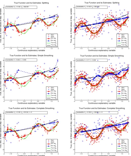
Example 4.2. (quadratic versus periodic regression)

−2 −1.5 −1 −0.5 0 0.5 1 1.5 2 −6

−4 −2 0 2 4 6

Continuous explanatory variable

True, obs. & fitted values of dep. variable

True Function and its Estimates: Splitting

Obs1 Obs2 Est−reg₁ Est−reg₂ True reg₁ True reg₂ bandwidths: h

1 = 0.124, h2 = 806.83

−2 −1.5 −1 −0.5 0 0.5 1 1.5 2

−6 −4 −2 0 2 4 6

Continuous explanatory variable

True, obs. & fitted values of dep. variable

True Function and its Estimates: Splitting

Obs1 Obs2 Est−reg

1 Est−reg

2

True reg₁

True reg₂

bandwidths: h₁ = 0.125, h₂ = 603.988

−2 −1.5 −1 −0.5 0 0.5 1 1.5 2

−6 −4 −2 0 2 4 6

Continuous explanatory variable

True, obs. & fitted values of dep. variable

True Function and its Estimates: Simple Smoothing

Obs1 Obs2

Est−reg₁

Est−reg₂

True reg₁

True reg 2 bandwidths: h = 0.232, λ = 0.009

−2 −1.5 −1 −0.5 0 0.5 1 1.5 2

−6 −4 −2 0 2 4 6

Continuous explanatory variable

True, obs. & fitted values of dep. variable

True Function and its Estimates: Simple Smoothing

Obs1 Obs2 Est−reg₁ Est−reg₂ True reg₁ True reg₂ bandwidths: h = 0.17, λ = 0.039

−2 −1.5 −1 −0.5 0 0.5 1 1.5 2

−6 −4 −2 0 2 4 6

Continuous explanatory variable

True, obs. & fitted values of dep. variable

True Function and its Estimates: Complete Smoothing

Obs1 Obs2 Est−reg

1 Est−reg

2 True reg 1 True reg 2 bandwidths: h₁ = 0.126, h₂ = 13.256, λ = 0.005

−2 −1.5 −1 −0.5 0 0.5 1 1.5 2

−6 −4 −2 0 2 4 6

Continuous explanatory variable

True, obs. & fitted values of dep. variable

True Function and its Estimates: Complete Smoothing

Obs1 Obs2 Est−reg

1 Est−reg

2 True reg 1 True reg₂ bandwidths: h₁ = 0.125, h₂ = 305.115, λ = 0

Figure 1.Example 4.1: Left panel, n=100and right panel, n=400. From top to bottom: Approach 1 (non-smoothing for the discrete variable), Approach 2 (local linear simple-smoothing), Approach 3 (local linear complete-smoothing).

simulation results are given in Figure 2 and Table 2. We find that in this case the difference between Approach 2 and the other two approaches is still present. From Table 2, we confirm the general comments given for Example 4.1: Approach 1 has the better performance than Approach 2, and Approach 3 is the more robust way in this scenario (with significantly better performances). In particular, note that even though the difference in curvatures between the two groups is not so extreme as in Example 4.1, the difference of performances is still substantial: the overall AMSE for Approach 2 is about 1.5 times larger than those for Approaches 1 and 3 whenn =50, and about twice as large for

n=100 and larger samples.

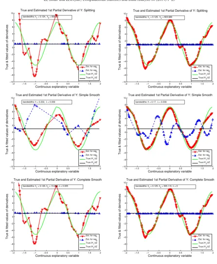
Consequences on the estimation of derivatives

The estimation of derivatives also has the phenomenon similar to what we just described. To save space, we only illustrate this for the case of the scenario described in Example 4.1. Figure 3 displays one typical sample and the resulting estimates of the first partial derivatives using the three approaches. This figure shows that the estimation of derivatives can be even more severely flawed by using the simple-smoothing approach. Indeed, as one can clearly see from Figure 3, with simple-smoothing technique, one obtained radically varying estimated curves of the derivatives for the group where their true values are constant. The problem sustains whether the total sample size is 100 or 400 (or more). This means that research conclusions, policy implications and, consequently, the real policy decisions based on such estimates may be misleading. Note that for the same example, the complete-smoothing approach produced much better results which are very close to the true values.

The Monte-Carlo experiment results based on the regression model (18) with more different choices of parameters can be found in working paper version of Li et al. (2013). As those results are similar, we omit them from the paper to save space.

5. Empirical application

In this section, we make an illustration of the phenomenon discussed above in the context of a real data set from the study by Kumar and Russell (2002), about patterns of convergence or divergence in economic growth in the World.2

We chose this data and the context because the topic of economic growth has remained interesting for a wide audience for centuries.

This data set consists of observations in 57 countries, containing the variables such as GDP, labour and capital of each country in 1965 and in 1990, and was originally extracted from the Penn World Tables. We will use this data to estimate regression relationship between the growth in GDP per capita of countries between 1965 and 1990 (response variable) and the initial levels of GDP per capita of these countries (continuous explanatory variable). Such a regression and many of its variations are often performed in empirical economic growth studies on convergence.

The interest of such studies often lies in that the growth rates of poorer countries are, on average, higher than those of the richer countries, and thus the poorer countries would eventually catch up with or converge to the levels of GDP per capita of the richer countries. This is often referred to as the (unconditional) “beta-convergence” phe-nomenon. Earlier works on this issue employed the parametric regression models. Some studies found that the slope coefficient (the “beta”) in such regressions is negative and significantly different from zero, which supports the “beta-convergence” hypothesis. However, other studies found that the “beta” is insignificantly different from zero (i.e., no convergence) or even positive (i.e., “beta-divergence”) and significantly different from zero for different samples or for distinct groups of countries within a sample or when additional explanatory variables are accounted for.3_{We next}

use the nonparametric regression method, which may give some useful insights. In particular, we apply the LLLS with the three approaches discussed above to the following regression relationship:

yi=m(zci,z d

i)+εi, i=1, . . . ,n

whereyiis growth in GDP per capita of countryibetween 1965 and 1990,zc_i is the natural log of GDP per capita

of countryiin 1965, whilezd

i is a discrete variable which will be defined later andεiis a stationary noise satisfying

E(εi|zc_i,zd_i)=0 and Var(εi|zc_i,zd_i)<∞a.s.

2_{This data set (or its extended version) was also used in many other applications, see, for example, Henderson and Russell (2005), Simar and}

Zelenyuk (2006), Henderson and Zelenyuk (2007) and Badunenko et al. (2008).

3_{For a recent review of this topic, see, for example, Maasoumi et al. (2007), Weil (2008) and references cited therein.}

−2 −1.5 −1 −0.5 0 0.5 1 1.5 2 −6

−4 −2 0 2 4 6

Continuous explanatory variable

True, obs. & fitted values of dep. variable

True Function and its Estimates: Splitting

Obs1 Obs2 Est−reg

1

Est−reg₂

True reg₁

True reg₂

bandwidths: h₁ = 0.125, h₂ = 932.951

−2 −1.5 −1 −0.5 0 0.5 1 1.5 2

−6 −4 −2 0 2 4 6

Continuous explanatory variable

True, obs. & fitted values of dep. variable

True Function and its Estimates: Splitting

Obs1 Obs2 Est−reg

1

Est−reg

2

True reg₁

True reg₂

bandwidths: h₁ = 0.125, h₂ = 252.406

−2 −1.5 −1 −0.5 0 0.5 1 1.5 2

−6 −4 −2 0 2 4 6

Continuous explanatory variable

True, obs. & fitted values of dep. variable

True Function and its Estimates: Simple Smoothing

Obs1 Obs2

Est−reg₁

Est−reg₂

True reg₁

True reg₂

bandwidths: h = 0.232, λ = 0.009

−2 −1.5 −1 −0.5 0 0.5 1 1.5 2

−6 −4 −2 0 2 4 6

Continuous explanatory variable

True, obs. & fitted values of dep. variable

True Function and its Estimates: Simple Smoothing

Obs1 Obs2 Est−reg₁ Est−reg₂ True reg₁ True reg

2

bandwidths: h = 0.17, λ = 0.039

−2 −1.5 −1 −0.5 0 0.5 1 1.5 2

−6 −4 −2 0 2 4 6

Continuous explanatory variable

True, obs. & fitted values of dep. variable

True Function and its Estimates: Complete Smoothing

Obs1 Obs2 Est−reg₁ Est−reg₂ True reg 1 True reg 2 bandwidths: h₁ = 0.125, h₂ = 610.34, λ = 0

−2 −1.5 −1 −0.5 0 0.5 1 1.5 2

−6 −4 −2 0 2 4 6

Continuous explanatory variable

True, obs. & fitted values of dep. variable

True Function and its Estimates: Complete Smoothing

Obs1 Obs2 Est−reg₁ Est−reg₂ True reg 1 True reg 2 bandwidths: h₁ = 0.126, h₂ = 28.982, λ = 0

Figure 2.Example 4.2: Left panel, n=100, and right panel, n=400. From top to bottom: Approach 1 (non-smoothing for the discrete variable), Approach 2 (local linear simple-smoothing), Approach 3 (local linear complete-smoothing).

−2 −1.5 −1 −0.5 0 0.5 1 1.5 2 −10 −8 −6 −4 −2 0 2 4 6 8 10

Continuous explanatory variable

True & fitted values of derivatives

True and Estimated 1st Partial Derivative of Y: Splitting

Est. for reg₁ Est. for reg

2

True ∂Y₁/∂Z True ∂Y₂/∂Z bandwidths: h₁ = 0.124, h₂ = 806.83

−2 −1.5 −1 −0.5 0 0.5 1 1.5 2

−10 −8 −6 −4 −2 0 2 4 6 8 10

Continuous explanatory variable

True & fitted values of derivatives

True and Estimated 1st Partial Derivative of Y: Splitting

Est. for reg₁

Est. for reg

2

True ∂Y₁/∂Z

True ∂Y

2/∂Z

bandwidths: h

1 = 0.125, h2 = 603.988

−2 −1.5 −1 −0.5 0 0.5 1 1.5 2

−10 −8 −6 −4 −2 0 2 4 6 8 10

Continuous explanatory variable

True & fitted values of derivatives

True and Estimated 1st Partial Derivative of Y: Simple Smooth

Est. for reg₁

Est. for reg₂

True ∂Y₁/∂Z True ∂Y

2/∂Z

bandwidths: h = 0.232, λ = 0.009

−2 −1.5 −1 −0.5 0 0.5 1 1.5 2

−10 −8 −6 −4 −2 0 2 4 6 8 10

Continuous explanatory variable

True & fitted values of derivatives

True and Estimated 1st Partial Derivative of Y: Simple Smooth

Est. for reg₁ Est. for reg₂ True ∂Y₁/∂Z True ∂Y

2/∂Z

bandwidths: h = 0.17, λ = 0.039

−2 −1.5 −1 −0.5 0 0.5 1 1.5 2

−10 −8 −6 −4 −2 0 2 4 6 8 10

Continuous explanatory variable

True & fitted values of derivatives

True and Estimated 1st Partial Derivative of Y: Complete Smooth

Est. for reg

1

Est. for reg₂ True ∂Y₁/∂Z True ∂Y₂/∂Z bandwidths: h₁ = 0.126, h₂ = 13.256, λ = 0.005

−2 −1.5 −1 −0.5 0 0.5 1 1.5 2

−10 −8 −6 −4 −2 0 2 4 6 8 10

Continuous explanatory variable

True & fitted values of derivatives

True and Estimated 1st Partial Derivative of Y: Complete Smooth

Est. for reg

1

Est. for reg₂ True ∂Y₁/∂Z True ∂Y₂/∂Z bandwidths: h₁ = 0.125, h₂ = 305.115, λ = 0

Figure 3.Derivative Estimates for Example 4.1: Left panel, n=100and right panel, n=400. From top to bottom: Approach 1 (non-smoothing for the discrete variable), Approach 2 (local linear simple- smoothing), Approach 3 (local linear complete-smoothing).

within the sample which have different regression relationships (in terms of intercept or slope or both). Indeed, in various existing studies, researchers often distinguish various groups of countries, allowing them to have different regression relationships. An objective grouping criterion often used in practice, for example, is an indicator whether

6.5 7 7.5 8 8.5 9 9.5 10 10.5 −1

0 1 2 3 4 5

Continuous explanatory variable

Observed data & fitted values of dep. variable

Estimation without discrete variable

Obs. Gr₁ Obs. Gr₂ Est−reg bandwidths: h = 0.212

6.5 7 7.5 8 8.5 9 9.5 10 10.5

−1 0 1 2 3 4 5

Continuous explanatory variable

Observed data & fitted values of dep. variable

Splitting

Obs. Gr

1

Obs. Gr

2

Est−reg₁ Est−reg₂ bandwidths: h

1 = 0.212, h2 = 1.215

6.5 7 7.5 8 8.5 9 9.5 10 10.5 −1

0 1 2 3 4 5

Continuous explanatory variable

Observed data & fitted values of dep. variable

Simple Smoothing

Obs. Gr

1

Obs. Gr₂ Est−reg₁ Est−reg

2

bandwidths: h = 1.006, λ = 0.024

6.5 7 7.5 8 8.5 9 9.5 10 10.5 −1

0 1 2 3 4 5

Continuous explanatory variable

Observed data & fitted values of dep. variable

Complete Smoothing

Obs. Gr₁ Obs. Gr₂ Est−reg₁ Est−reg

2

bandwidths: h₁ = 0.293, h₂ = 1.203, λ = 0.005

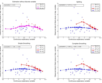
Figure 4. Illustration with GDP data. From left to right and top to bottom, Panel (a): Approach 0 (without the discrete variable), Panel (b): Approach 1 (non-smoothing for the discrete variable), Panel (c): Approach 2 (local linear simple-smoothing), Panel (d): Approach 3 (local linear complete-smoothing).

a country is an OECD member or not (e.g., Racine et al., 2006; Simar and Zelenyuk, 2006; Maasoumi et al., 2007; Henderson and Zelenyuk, 2007), and so we also use this as our discrete variable,zd

i, which has the value 1 if country

iwas a member of the OECD in the year 1965 and zero otherwise.4

In panel (b) of Figure 4, we give the LLLS estimated curves by using Approach 1 (i.e., separate estimation for each group withhchosen via CV for each group separately), and one can see that the estimated relationships for the two groups are very different not only in the intercept but also in the slope. Specifically, note that the relationship for the larger non-OECD group is virtually flat, with very slight inverted-U-shape curvature. On the other hand, note that the relationship for the smaller OECD group has a more pronounced inverted-U-shape curvature (or rather “inverted hockey-stick” shape). Note that such curvature may suggest an important economic implication. It hints that the OECD countries with very low initial GDP per capita are expected to have higher growth rates in GDP per capita than those with very high initial GDP per capita, yet the highest rates are expected to be not at the lowest level of GDP per capita but somewhat larger.

In panel (c) of Figure 4, we present the LLLS estimated curves by using Approach 2 (i.e., local linear simple-smoothing withhandλselected jointly via the CV method for the entire sample). One can see that the estimated

4_{In a detailed analysis, one may want to condition for many other potentially important explanatory variables, yet we will limit our illustration}

relationships are also very different between the two groups. The relationship for the non-OECD group has a slightly more pronounced inverted-U-shape curvature, although it still remains relatively flat. On the other hand, the rela-tionship for the OECD group has much less curvature than that in panel (b), and it is not an inverted-U-shape at all. Hence, Approach 2 suggests that for the OECD countries there is an almost linear and negative relationship between the growth in GDP per capita and the initial level of GDP per capita. In other words, with the local linear simple-smoothing approach, we get some under-simple-smoothing for the larger group and over-simple-smoothing for the smaller group compared with panel (b) by the separate estimation approach. This is similar to what we have observed from the simulated examples.

Some additional insight is provided by the local linear complete-smoothing method (Approach 3), where we allow for each group identified by the discrete variable to have its own bandwidth but also smooth the discrete variable and so use the full sample in one estimation. Panel (d) of Figure 4 visualizes the estimated curves by using Approach 3 and one can see that it gives almost identical results to those by using Approach 1, which is similar to what we have observed from the simulation studies. In this small data set, we can also find that the left-most observation in group 1 might be an outlier, and so omitting it when using Approaches 1 and 3 may produce results very similar to Approach 2. However, it might be the case that there are other data points not available in our sample which are close to this left-most observation in group 1 and including them would make the invertedU-shape curvature even more pronounced. Since we do not know the true relationship, unlike in the simulated examples, it is difficult to judge which of these two arguments is likely to be right or wrong, which is beyond the scope of this paper. Since Approach 3 encompasses the other two approaches by taking the best features from each, and that our simulations suggested that Approach 3 was more robust than the other two, Approach 3 appears to be more reliable for a practitioner to trust in this context and perhaps in general, whenever it is computationally feasible.

Finally, it might be worth emphasizing again that in this section we had not intended to resolve the puzzles of economic growth across countries as such a study would require a larger data set and more variables. Our aim was just to give a concise and vivid illustration of the phenomenon we discussed above and, in particular, to compare the three approaches, not only for simulated data sets, but also for a real data set, in a context that appears to be interesting for a wide audience.

6. Conclusion

In this article we have pointed out and illustrated that the reduction in variance or the efficiency gain due to smooth-ing of the discrete regressors with common bandwidth for the continuous variables across groups, as is frequently done in applied studies, can be well outweighed by the substantial bias introduced due to this simple-smoothing approach, both for small and for relatively large sample cases. For such cases, even fully separate estimation for each group, if feasible, might be preferred. We have shown that the complete-smoothing technique by allowing different bandwidths for the continuous variables in each group, could overcome this difficulty and so is more robust than the existing smoothing methods. In general, whether it is better to smooth or not to smooth the discrete variable, or whether “the bias beats the variance”, essentially depends on the degree of difference of the DGPs in different groups: curvatures of the regression relationship, variation in the error term for each group, variation in the continuous regressors, size or proportion of one group relative to another in the sample, and so on. The more robust complete-smoothing approach proposed in this paper is indeed a generalization of the seminal work by Racine and Li (2004), but at a cost of slightly more computational complexity. When using the simple-smoothing method, one automatically (or implicitly) imposes the assumption of a similar degree of smoothness of the regression relationships for different groups of the sample identified by the discrete variables, which might be far from reality. As we illustrated in both simulated and empirical examples, such a restriction can significantly deteriorate estimation results, increasing bias in the estimates of the true regression relationship. Such a problem can also substantially or even radically distort estimates of derivatives and the related estimates of marginal effects and elasticities, which are used to draw policy implications. It is also important to recognize that even from a theoretical point of view, the simple-smoothing of the discrete variable is preferable and offers a suitable solution to the problem, it is still an open question in practice for some real data sets, whether we have to smooth or not to smooth the discrete variables, particularly when the computational cost of the extended method is prohibitive.

A possible future topic is to extend the methodology to the case that the dimensions of both discrete and continuous covariates are multivariate. To avoid the curse of dimensionality issue in nonparametric estimation, inspired by the

recent work of Li et al. (2013), we may consider the following regression model with functional coefficients:

Yi=βτ(Zi)Xi+εi=βτ1(Zi)Xic+β τ

2(Zi)Xid+εi,

whereXi =(Xc_i,X_id) withXc_i ∈ Rr1 being continuous andXd_i being ar2-dimensional discrete vector,β1(·) andβ2(·)

are functional coefficients with dimensionsr1andr2, respectively, andZi=(Zc_i,Z_id) withZ_icbeing univariate

contin-uous covariate andZd

i being univariate discrete covariate. It would be interesting to apply the local linear complete

smoothing to estimate the functional coefficients in the above modelling framework and study its asymptotic theory and empirical application.

Another possible future work is to develop and justify a method (a specification test or a rule of thumb) that would help justifying a decision whether to smooth or not to smooth over some or all discrete variables. The issue of relevance of some categorical predictors in nonparametric regressions has been analyzed in Racine et al. (2006) by considering the hypothesis testing problem ofλ=1. However, to the best of our knowledge, nothing has been done for the other extreme of the scale (λ=0), including the issue of common bandwidths for the continuous variables. It would be also interesting to investigate whether the complete-smoothing method we proposed in this paper can also improve the performance of various tests that employ the simple-smoothing method (see, for example, Racine et al., 2006; Hsiao et al., 2007).

7. Acknowledgements

We would like to thank the editor, associate editor, and two referees for their helpful comments, which greatly im-proved the previous version of the paper. Thanks also go to Peter C. B. Phillips, JeffRacine and other colleagues who commented on this paper and participants of various conferences and seminars where this work was presented. The second author and the third author acknowledge the financial support from ARC Discovery Grant (DP130101022), the IAP Research Network P7/06 of the Belgian State (Belgian Science Policy) and the School of Economics and CEPA of The University of Queensland. Only the authors and not the above mentioned institutions or people remain responsible for the views expressed.

Appendix A. Assumptions

In this appendix, we give the regularity assumptions which are sufficient to derive the asymptotic theory of the proposed approach in Section 3.

Assumption 1. Let_{(Yi,Z_ic,Z_id)}be independent and identically distributed (i.i.d.) as (Y,Zc,Zd), and the error term εihave the (2+δ) moment withδ >0.

Assumption 2. LetK(·) be a continuous and symmetric probability density function with a compact support.

Assumption 3. The conditional density function ofZcfor givenZd,f(zc_|zd), is bounded away from infinity and zero

forzc_{∈ Z}candzd =zd(1) orzd(2), whereZc

is the compact support ofZc. Meanwhile,m(·,zd),σ2(·,zd) and

f(·|zd) are twice continuously differentiable onZc

forzd =zd(1) orzd(2), whereσ2(zc,zd)=Var[ε_|Z=(zc,zd)].

Assumption 4. Let the bandwidthsh(1),h(2) andλsatisfy

h(1)_∨h(2)_→0, hnh(1)i_∧hnh(2)i_{→ ∞} and λ=O(h2(1)_∧h2(2)).

Assumption4′. Let the bandwidthsh(1) andh(2) satisfy

h

n2ǫ−1h(1)i_∧hn2ǫ−1h(2)i_{→ ∞}, ǫ <(δ+1)/(2+δ),

whereδis defined in Assumption 1. Furthermore, [nh4_(1)]

∧[nh4_(2)]

In Assumption 1, we impose the i.i.d. condition on the observations, which has been widely used in the literature on nonparametric estimation with both categorical and continuous data, see, for example, Li and Racine (2004) and Racine and Li (2004). We conjecture that our asymptotic theory can be generalized to some stationary and weakly dependent (such asβ-mixing dependent) processes at the cost of more lengthy proofs. Assumption 2 imposes some mild conditions on the kernel function, and several commonly-used kernel functions such as the uniform kernel and the Epanechnikov kernel satisfy these conditions. Assumption 3 imposes some smoothness conditions on the conditional density function, conditional regression function and conditional variance function, which are necessary when the LLLS estimation approach is applied. Assumptions 4 and 4′impose some restrictions on the bandwidths. In particular, Assumption 4′is critical to apply the uniform consistency results of the nonparametric kernel estimators.

Appendix B. Proofs of the asymptotic results

We next give the proofs of the asymptotic results stated in Section 3.

Proof of Theorem 3.1. Let

∆n(1) =

n X

i=1

"

1 (Z_ic₋zc) (Z_ic₋zc) (Z_ic₋zc)2

#

Λλ(Zid,z d

)Kh(1)(Zic−z c

)InZ_id=zd(1)o,

∆n(2) =

n X

i=1

"

1 (Z_ic₋zc) (Z_ic₋zc) (Z_ic₋zc)2

#

Λλ(Zid,z d

)Kh(2)(Zic−z c

)InZ_id=zd(2)o,

Ωn(1) =

n X

i=1

₁

Z_ic₋zc

e

YiΛλ(Zid,z d

)Kh(1)(Zic−z c

)InZ_id=zd(1)o,

Ωn(2) =

n X

i=1

₁

(Z_ic₋zc)

e

YiΛλ(Zid,z d

)Kh(2)(Zic−z c

)InZ_id=zd(2)o,

whereeYi=Yi−m(zc,zd)−m′(zc,zd)(Z_ic−zc),m′(zc,zd) is the first-order partial derivative ofm(·,·) with respect tozc,

and lete2(1) be a 2-dimensional column vector with the first element being 1 and elsewhere 0.

By some elementary calculations, we can show that

ζ(zc,zd) :=_em(zc,zd)−m(zc,zd)=eτ₂(1)∆+_nΩn, (B.1)

where∆n= ∆n(1)+ ∆n(2),Ωn= Ωn(1)+ Ωn(2) and∆+n is the Moore-Penrose inverse matrix of∆n.

We first consider the case ofzd =zd(1). Note that for this case,

∆n(1)=

n X

i=1

"

1 (Z_ic₋zc) (Z_ic₋zc) (Z_ic₋zc)2

#

Kh(1)(Zci −z c

)InZd_i =zd(1)o,

and

∆n(1)=E[∆n(1)]+ ∆n(1)−E[∆n(1)].

By Assumptions 2–4 and standard argument, we can prove

1

nH

+

1E[∆n(1)]H1+=p1f(zc|zd(1))∆(K)+oP(1), (B.2)

whereH1=diag(1,h(1)),p1=P(Zd=zd(1)), and∆(K)=diag(1, µ2). Furthermore, we can show that

Var

₁

nH

+

1∆n(1)H1+

=O 1

nh(1)

=o(1),

asnh(1)_{→ ∞}, which implies that 1

nH

+

1

∆n(1)−E[∆n(1)]

H+₁ =oP(1). (B.3)

Equations (B.2) and (B.3) lead to

1

nH

+

1∆n(1)H1+=p1f(zc|zd(1))∆(K)+oP(1). (B.4)

On the other hand, whenzd=zd(1), note that

∆n(2) = λ

n X

i=1

"

1 (Zc i −z

c₎

(Zc i −z

c_{) (Z}c i −z

c₎2

#

Kh(2)(Zci −z c

)InZd_i =zd(2)o.

By the conditionλ=O(h2₍₁₎

∧h2_{(2)) in Assumption 4, following the proof of (B.4),∆}

n(2) is dominated by∆n(1),

which implies that

1

nH

+

1∆nH+1 =

1

nH

+

1∆n(1)H1++oP(1)=p1f(zc|zd(1))∆(K)+oP(1). (B.5)

We next look intoΩnfor the case ofzd =zd(1). Observe that

Ωn(1) =

n X

i=1

₁

Z_ic₋zc

e

YiKh(1)(Zci −z c

)InZd_i =zd(1)o,

Ωn(2) = λ

n X

i=1

₁

(Zc_{i −}zc)

e

YiKh(2)(Zic−z c

)InZ_id=zd(2)o.

Furthermore, by the definition of the model, we can show that

Ωn(1) =

n X

i=1

₁

Zc i −z

c

ρ1(Zci)Kh(1)(Zci −z c

)InZd_i =zd(1)o

+

n X

i=1

₁

Zc i −z

c

εiKh(1)(Zci −z c

)InZd_i =zd(1)o

=: Ωn(1,1)+ Ωn(1,2),

whereρ1(Z_ic)=m(Z_ic,zd(1))−m(zc,zd(1))−m′(zc,zd(1))(Z_ic−zc), and

Ωn(2) = λ

n X

i=1

₁

Zc i −z

c

ρ2(Zic)Kh(2)(Zic−z c

)InZ_id=zd(2)o

+λ

n X

i=1

₁

Zc i −z

c

εiKh(2)(Zic−z c

)InZ_id=zd(2)o

=: Ωn(2,1)+ Ωn(2,2),

whereρ2(Zci)=m(Z c i,z

d₍₂₎₎

−m(zc_,zd₍₁₎₎

−m′_(zc_,zd_(1))(Zc i −z

c_{). As E(ε}

|Z)=0 a.s.,Ωn(1,1) andΩn(2,1) contribute

to the asymptotic bias of the local linear estimator with complete smoothing. By standard argument for the local linear smoothing, we can show that

1

nH

+

1Ωn(1,1)=

1 2p1f(z

c

|zd(1))µ2m′′(zc,zd(1))h2(1)e2(1)+OP(h4(1)). (B.6)

On the other hand, notice that

ρ2(Zci)=m(Z c i,z

d

(2))₋m(zc,zd(1))₋m′(zc,zd(1))(Zc_{i −}zc)_≈m(zc,zd(2))₋m(zc,zd(1)).

We can thus prove that

1

nH

+

1Ωn(2,1)=λ(1−p1)f(zc|zd(2))

h