Preparational Uncertainty Relations for N Continuous Variables

This is a repository copy of Preparational Uncertainty Relations for N Continuous

Variables.

White Rose Research Online URL for this paper:

http://eprints.whiterose.ac.uk/105699/

Version: Accepted Version

Article:

Kechrimparis, Spyridon and Weigert, Stefan orcid.org/0000-0002-6647-3252 (2016)

Preparational Uncertainty Relations for N Continuous Variables. Mathematics. pp. 1-17.

ISSN 2227-7390

https://doi.org/10.3390/math4030049

[email protected] https://eprints.whiterose.ac.uk/ Reuse

This article is distributed under the terms of the Creative Commons Attribution (CC BY) licence. This licence allows you to distribute, remix, tweak, and build upon the work, even commercially, as long as you credit the authors for the original work. More information and the full terms of the licence here:

https://creativecommons.org/licenses/

Takedown

If you consider content in White Rose Research Online to be in breach of UK law, please notify us by

Preparational Uncertainty Relations

for

N

Continuous Variables

Spiros Kechrimparis and Stefan Weigert Department of Mathematics, University of York

York, YO10 5DD, United Kingdom

29 June 2016

Abstract

A smooth function of the second moments ofNcontinuous variables gives rise to an uncertainty relation if it is bounded from below. We present a method to sys-tematically derive such bounds by generalizing an approach applied previously to a single continuous variable. New uncertainty relations are obtained for multi-partite systems which allow one to distinguish entangled from separable states. We also investigate the geometry of the “uncertainty region” in the N(2N+1)-dimensional space of moments. It is shown to be a convex set for any number continuous vari-ables, and the points on its boundary found to be in one-to-one correspondence with pure Gaussian states of minimal uncertainty. For a single degree of freedom, the boundary can be visualized as one sheet of a “Lorentz-invariant” hyperboloid in the three-dimensional space of second moments.

1

Introduction

Uncertainty relations express limitations on the precision with which one can measure specific properties of a quantum system, such as position and momentum of a quantum particle. These relations come in different flavours. They may express the inability to pre-parea quantum system in a state for which incompatible properties possess exact values. Alternatively,error-disturbanceuncertainty relations refer to the constraints encountered when attempting to extract precise values through measurements on a single system. Both cases point to the uncertainty inherent in the quantum description of the world.

Heisenberg was the first to realize, in 1927, that uncertainty relations exist for quan-tum systems [1]. His physical arguments were quickly developed by Kennard [2], Weyl [3], Robertson [4] and Schr ¨odinger [5]. Except for Heisenberg’s paper, the focus of these contributions was on preparational uncertainty, not yet clearly distinguished from surement uncertainty. Only in 1965, Arthurs and Kelly presented a model of joint mea-surement of position and momentum [6], laying the foundations for interest in error-disturbance uncertainty relations which has grown considerably over the last two

cades. Different approaches rely on different concepts of error which has led to lively debates [7, 8].

In recent years, the discussion of uncertainty relations has turned from conceptual aspects to applications, in line with the overall thrust of quantum information. For ex-ample, the first protocol of quantum cryptography, known as BB84 [9], is based on pairs of mutual unbiased bases which are known to come with maximal preparational uncer-tainty. It is also possible to use variance-based uncertainty relations to formulate criteria to detect entangled states of bi-partite systems [10, 11].

This work investigates the structure of preparational uncertainty relations in quan-tum systems with more than one continuous variable, i.e. N ≥ 2. Examples are given by a point particle moving in a plane (N = 2) or in three-dimensional space (N = 3); alternatively, one may considerNparticles each moving along a real line, each with con-figuration spaceR_{. Our main goals are (i) to obtain lower bounds for given smooth}

functions depending on theN(2N+1)second moments of a system with Ncontinuous variables, (ii) turn these bounds into criteria which enable us to detect entangled states, and (iii) to understand the geometric structure of uncertainty functionals in the space of second moments, spanned by the independent elements of the covariance matrix.

Using a variational technique originally introduced by Jackiw [12], we will generalize an approach which has been carried out successfully for quantum systems with a single particle-type degree of freedom, i.e.N =1 [13]. Encouraged by the new uncertainty rela-tions obtained in this way for a single continuous variable, we are particularly interested in the possibility to create inequalities which are capable to detect entangled states in sys-tems with two or more continuous variables. Tools to detect entanglement are crucial for the implementation of any protocol in quantum information which relies on entangled states. For continuous variables, quantum optical methods are available to reliably check variance-based entanglement criteria, allowing one to verify that a required entangled state has indeed been created [14, 15, 16].

2

Lower bounds of uncertainty functionals

2.1 Extrema of uncertainty functionals

To describe a quantum system of continuous variables withNspatial degrees of freedom, one associatesNpairs of canonical operators obeying the commutation relations

[qˆk, ˆpk′] =i¯hδ_kk′, [qˆ_k, ˆq_k′] = [pˆ_k, ˆp_k′] =0 , k,k′ =1, . . . ,N. (1)

We will arrange the momentum and position operators of thek-th degree of freedom, ˆpk and ˆqk, respectively, into a column vector ˆz,

ˆz⊤= (p1ˆ , ˆq1, . . . , ˆpN, ˆqN) ≡(z1ˆ , ˆz2, . . . , ˆz2N−1, ˆz2N), (2)

with 2Ncomponents ˆzµ,µ= 1, . . . , 2N. The pure states of the quantum systems consid-ered here are represented by unit vectors |ψi ∈ H_{, in an infinite-dimensional Hilbert} spaceH_{. Of the(2N)}2_{second moments}

cµν = 1

2hψ| zµˆ zνˆ +zµˆ zνˆ

|ψi, µ,ν=1, . . . , 2N, (3)

only N(2N+1)are independent. We assume (without loss of generality) that all first moments vanish, which follows from the invariance of the second moments under rigid phase-space translations. The second momentscµν form the covariance matrix C associ-ated with the pure state|ψi.

With k = 1, . . . ,N, and for µ = ν = 2k−1 (µ = ν = 2k) one obtains the variance of momentum (position) of thek-th degree of freedom, while forµ = 2k,ν = 2k−1 we obtain their covariance; all other values of the indicesµ,ν, correspond to moments which mix different degrees of freedom. Occasionally, we will denote the variances of thek-th momentum and position withxkandyk, respectively, and their covariance bywk.

Given a real function of the second moments forNcontinuous variables, f :RN(2N+1)

→ R_{, we wish to establish whether it has a non-trivial lower bound b. If it does, the}

statement f _≥ bprovides an uncertainty relation.

Following an idea of Jackiw [12] (see also [17, 18, 19]), we define anuncertainty func-tionalassociated with the function f by

J[ψ] = f ∆2p1,∆2q1,Cp1q1, . . .Cp1p2,Cp1q2, . . .

−λ(_hψ_|ψ_{i −}1),

= f(x1,y1,w1, . . . ,c13,c14, . . .)₋λ(_hψ|ψi −1), (4)

operators. Let us briefly spell out the derivation in the more general setting.

First, we compare the value of the functionalJ[ψ]in the state|ψ+εi=_|ψi+ε|eiwith its value in the state_|ψ_i, where_|e_{i ∈} H _{is an arbitrary normalised state. Expanding it} up to second order in the small parameterε, we find

J[ψ+ε] = J[ψ] +εDεJ[ψ] +O ε2, (5)

where the expression

Dε =_he|_δδ hψ| +

δ

δ|ψi|ei, (6)

denotes a Gˆateaux derivative. The stationary points of the functional are characterised by the vanishing of the first-order term in the expansion (5),

DεJ[ψ] =_he_|

δ

δhψ|f(x1,y1,w1, . . . ,c13,c14, . . .)−λ|ψi

+c.c.=0 . (7)

More explicitly, this condition reads

he|

∑

∂f ∂cµν

δcµν δ_hψ_|

−λ|ψi !

+c.c.=0 , (8)

where the sum runs over the values 1≤ µ ≤ 2Nandµ ≤ ν ≤ 2N. Since Eq. (8) should hold for arbitrary variations of the ket|eiand its dualhe|(which are independent), the expression in round brackets as well as its complex conjugate must vanish identically.

The functional derivatives of the second moments are δcµν

δhψ| ≡ 1

2 zµˆ zνˆ +zνˆ zµˆ

|ψi, (9)

resulting in anEuler-Lagrange-type equation,

∑

1

2 zµˆ zνˆ +zνˆ zµˆ ∂f

∂cµν −λ !

|ψi=0 . (10)

The value of the multiplierλcan be found by multiplying this equation with the brahψ| from the left and solving forλ. Substituting its value back into Eq. (10), one finds the nonlinear eigenvector-eigenvalue equation,

∑

1

2 zµˆ zνˆ +zνˆ zµˆ ∂f

∂cµν|ψi=_µ

∑

∂cµν|ψi, (11)

or, in matrix notation,

ˆ

z⊤Fzˆ_|ψi=Tr(C F)|ψi, (12)

the standard convention to denote partial derivatives by subscripts. As an example, the eigenvalue equation becomes, forN=2,

2

∑

k=1

fxkpˆ 2 k+ fykqˆ

2 k+

fwk

2 (qˆkpˆk+pˆkqˆk)

+ fc13p1ˆ p2ˆ +. . .+ fc24q1ˆ q2ˆ

! |ψ_i=

= 2

∑

k=1

xkfxk+ykfyk+wkfzk

+c13fc13+. . .+c24fc24

! |ψ_i.

(13)

Note that Eq. (12) is generally non-linear in the state_|ψ_isince the second moments and the partial derivatives off are functions of expectation values in the state|ψi. As we will show in next section, one can nevertheless solve Eq. (12), given a number of assumptions.

2.2 Consistency conditions

To solve Eq. (12), we initially assume that the matrixFof partial derivatives isconstant, i.e. we suppress its dependence on the state |ψi. If we further require that F is posi-tive definite, then Williamson’s theorem [21, 22] guarantees the existence of a symplectic matrixΣ_{that putsFinto a diagonal form, i.e.}

F=Σ⊤DΣ_{, (14)}

where the diagonal matrixDis defined byD=diag(λ1,λ1, . . . ,λN,λN), and the positive real numbersλk > 0, k = 1, . . . ,N, are the symplectic eigenvaluesof F [23, 24, 22]. We recall that a symplectic matrix of order 2N satisfiesΣ⊤Ω Σ = Ω_{, where}Ω _{is uniquely}

determined by the commutation relations,[zµˆ , ˆzν] =i¯hΩ_µν,µ,ν=1, . . . , 2N.

Multiplying both sides of Eq. (12) with the metaplectic unitary operator ˆS† from the left, defined by the relation

Σ_{zˆ = S}ˆ_ˆzSˆ†_{, (15)}

we find that its left-hand-side can be expressed as

ˆ

S†zˆ⊤FzˆSˆSˆ†|ψi= Sˆ†zˆ⊤SˆFSˆ†zˆSˆ Sˆ†|ψi

= Σ−1zˆ⊤Σ⊤DΣ Σ−1_{zˆ S}ˆ†_{|ψi. (16)}

Thus, Eq. (12) simplifies to

ˆ

z⊤Dzˆ Sˆ†|ψi=Tr(C F)Sˆ†|ψi , (17)

which can be written as N

∑

k=1 λk

ˆ p2_k+qˆ2_k

2 !

ˆ

S†|ψi= 1

2Tr(C F)

ˆ

Thus, we have transformed the quadratic operator on the left-hand-side of Eq. (12) into a Hamiltonian operator given by a sum ofNdecoupled harmonic oscillators. The solutions of Eq. (18) are given by tensor products of number states for each degree of freedom,

|ψ_i=Sˆ(_|n1_{i ⊗}. . ._{⊗ |}nNi)≡Sˆ N

O

k=1 |nki

!

. (19)

Note that the constraint 1

2Tr(C F) = N

∑

k=1 λk

nk+ 1

2

¯

h, (20)

must be satisfied by all potential extremal states.

Recall that we have treated the matrix elements of the matrix F introduced in Eq. (12) as constants, on which the unitary transformation ˆSand hence the states|ψiin Eq. (19) now depend. To achieve consistency, we determine the expectation value of the covariance matrix in the solution|ψi. A set of coupled equations in matrix form results for the extremal second moments, which we will call theconsistency conditions. Explicitly, we find

C=_hψ|_Cˆ_{|ψi ≡} 1

2hψ|

ˆ

z_⊗zˆ⊤+zˆ_⊗zˆ⊤⊤

|ψi

= 1 2

N

O

k=1 hnk|

! ˆ S†

ˆ

z_⊗zˆ⊤+zˆ_⊗zˆ⊤⊤

ˆ S

N

O

k′=1 |nk′i

!

, (21)

where ˆz_⊗zˆ⊤ denotes the Kronecker product of the column vector ˆzwith its transpose, ˆ

z⊤. Using the identity (15) in the form Σ−1_{zˆ = Sˆ}†_{ˆzSˆ, we can express the covariance} matrix in the form

C=Σ−11

2

N+N⊤(Σ−1₎⊤_{, (22)}

with the matrix

N=

N

O

k=1 hnk|

! ˆ

z_⊗zˆ⊤

N

O

k′=1 |nk′i

!

, (23)

having elements

Nµν =_hn1, . . . ,nN|zµˆ zνˆ |n1, . . . ,nNi, µ,ν=1, . . . , 2N. (24)

Recalling that the components of the vector ˆzare position and momentum operators, it is not difficult to see that the only non-zero matrix elements ofNare on its diagonal, i.e.

N=¯hdiag

n1+ 1

2,n1+ 1

2, . . . ,nN+ 1 2,nN+

1 2

(25)

consistency conditionsforNcontinuous variables,

C=Σ−1_N(Σ−1₎⊤_{. (26)}

These conditions select the extrema that are compatible with the specific function of the second moments considered. The constraint given in (20) can be rewritten as

Tr(C F) =Tr(D N), (27)

and it is easy to check that this condition is trivially satisfied if the consistency conditions (26) hold.

The take-away message from the conditions (26) can be summarised as follows: a function f of the second moments of N positions and momenta has an extremum in a pure state |ψiif there exists a symplectic matrixΣ_{that diagonalises the covariance matrixCand, at the same}

time, the transpose of its inverse, Σ−1⊤

, diagonalises the matrixFof the partial derivatives of the function f.

According to (26), the determinant of the covariance matrix for extremal states of the uncertainty functionalJ[ψ]takes the value

detC= N

∏

k=1

nk+1 2

2 ¯

h2. (28)

Clearly, the minimum is achieved when each oscillator resides in its ground state,

detC_≥

¯ h 2

2N

, (29)

corresponding ton1=. . .=nN =0 in Eq. (28).

No pure N-particle state can give rise to a covariance matrixCviolating the inequal-ity (29). This universally valid constraint generalizes the single-particle inequalinequal-ity de-rived by Robertson and Schr ¨odinger toNparticles, expressing it elegantly as a condition on the determinant of the covariance matrix of a state. Supplying (28) with the lower-dimensional Robertson-Schr ¨odinger-type inequalities that need to be obeyed in by each subsystem of dimension 2 toN−1, we get the general uncertainty statement for more than one degrees of freedom, usually expressed in the form,

C+i¯h

2Ω≥0 . (30)

Alternatively, this requirement can be expressed in terms of inequalities for the symplec-tic eigenvalues of the covariance matrix [22, 24].

Σ_{=SγGb, with symplectic matricesGbandSγgiven by}

Gb=

1 0 b 1

!

, and Sγ = e

−γ ₀

0 eγ !

, (31)

respectively, and real parameters

b= fw 2fy ∈

R _{and γ=} 1

2ln

fy √

detF

∈R_{. (32)}

The consistency conditions now take the simple form

C=Σ−1_N(Σ−1₎⊤_=G−1

b S−γ1(S−γ1)⊤(G−b1)⊤h¯

n+1 2

= F−1¯h

n+ 1 2

√

detF (33)

or finally,

F C

√

detF = ¯h

n+ 1

2

I, n∈N_{0. (34)}

Therefore, the formalism developed here correctly reproduces the findings of [13].

3

Inequalities for two or more continuous variables

3.1 Inequalities without correlation terms

Let us now examine the consistency conditions for more than one degree of freedom while allowing only product states. Correlations between the degrees of freedom be-ing absent, the functional will only depend on the local second moments, that is, f ≡ f(x1,y1,w1, . . . ,xN,yN,wN); the 2N(N−1)moments mixing the degrees of freedom are always zero in a separable state. For simplicity, we only considerN = 2 in some detail, the generalisation toN>_{2 being straightforward.}

Using matricesGb andSγ defined in (31), we construct two symplectic matricesS1 andS2as follows,

Σ₁₌ Sγ1Gb1 0

0 I

!

and Σ₂₌ I 0

0 Sγ2Gb2

!

. (35)

Their product,Σ₌Σ₁Σ_{2describes the action of the factorised unitary operator}

ˆ

S=S1ˆ ⊗S2ˆ , (36)

when solving the eigenvalue equation (12). The consistency conditions become

C=Σ−1_N(Σ−1₎⊤₌ Σ−1₍Σ−1₎⊤_N=F−1

with

Fpr =

F1/√detF1 0

0 F2/√detF2 !

, (38)

so that we finally obtain

FprC=N; (39)

in Eq. (38), the 2×2 matricesFk,k=1, 2, denote the collection of partial derivatives of the functionf with respect to the moments of thek-th degree of freedom. Therefore, the con-sistency conditions for functionals of product states reduce to a pair of one-dimensional ones which must be solved simultaneously.

The generalisation toNdegrees of freedom is straightforward: for each extra degree of freedom, a matrixFk/√detFk must be added to the diagonal of the block matrixFpr. After introducing the suitably generalized matricesCandN, Eqs. (39) describe the con-sistency conditions for separable quantum states. It is often useful to express Eq. (39) as

xkfxk =ykfyk, 2wkfyk = −xkfwk, xkyk−w 2 k = ¯h2

nk+

1 2

, (40)

withk=1, . . . ,N.

The simplest example of a factorized uncertainty relation is given by the product of two one-dimensional Robertson-Schr ¨odinger inequalities, following from the functional

f(x1,y1,w1,x2,y2,w2) = (x1y1₋w2₁)(x2y2₋w2₂), (41)

The resulting inequality,

∆2p1∆2q1−C2_p1q1 ∆2p2∆2q2−C2_p2q2≥

¯ h 2

4

, (42)

corresponds to the boundary described by Eq. (29) in the absence of correlations, to be discussed in more detail in Sec. 4. Note that this inequality is only invariant under Sp(2,R_)⊗Sp(2,R_{)transformations instead of the those of Sp(4,}R_{)group that leave}

in-variant the Robertson-Schr ¨odinger-type inequality for two degrees of freedom. However, the matrix inequalityC+iΩ_{h¯/2 ≥ 0 is invariant under any symplectic transformation}

and serves as the required generalisation. Starting from the functional

and after solving (39), we arrive at the inequality

∆2_p1∆2_q1∆2_p2∆2_{q2 ≥}

¯ h 2

4

+C2_p1q1C2_p2q2, (44)

which cannot be obtained by a combination of inequalities forN = 1. It isstrongerthan the (factorized) “Heisenberg”-type inequality for more than two observables,

∆p1∆q1∆p2∆q2_≥

¯ h 2

2

, (45)

first mentioned in a paper by Robertson [25], butweakerthan (42). An inequalityI1is said to be weaker than the inequalityI2if less states saturateI1thanI2.

Mixing products of variances related to different degrees of freedom also leads to non-trivial inequalities such as

a ∆2_p1∆2_q2n

+b ∆2_p2∆2_q1n

≥2√ab

¯ h 2

2n

, a,b>_{0 . (46)}

Fora=b=1 andn=1, one obtains

∆_p1∆_q2+∆_p2∆_{q1 ≥h¯,}

which resembles the inequality for the sum of two one-dimensional Heisenberg inequal-ities,

∆_p1∆_q1+∆_p2∆_{q2 ≥h¯, (47)}

but differs fundamentally from it.

3.2 Inequalities with correlation terms

Dropping the limitation to product states, we now turn to functionals that involve terms to which different degrees of freedom contribute. To begin, let us consider a linear com-bination of second moments,

f ∆2_{p1, . . . ,Cq1q2}

= a ∆2_p1+∆2_q1

+b ∆2_p2+∆2_q2

+c Cp1p2−Cq1q2

,

for which the matrixFtakes the form

F=



    

a 0 c_{/2 0} 0 a 0 −c_/2 c_{/2 0 b 0}

0 ₋c_{/2 0 b} 

    

. (48)

diagonal form is given by (cf. [26]): Σ₌      

σ+ 0 σ− 0

0 σ+ 0 −σ−

σ− 0 σ+ 0

0 −σ− 0 σ+

      , (49) where

σ±=

s

a+b±√y

2√y , and y= (a+b)

2_−c2_{. (50)}

The consistency conditions (26) can be solved in closed form, leading to the covariance matrix at the extrema

C=      

∆2_p(e)

1 0 C

(e)

p1p2 0

0 ∆2_q(e)

1 0 C

(e)

q1q2

C(pe1)p2 0 ∆

2_p(e)

2 0 0 C(qe1)q2 0 ∆

2_q(e) 2       , (51)

with elements explicitly given by

∆2p(₁e) =∆2q₁(e) = (n1−n2)h¯

2 +

(a+b)(n1+n2+1)h¯

2p(a+b)2_−c2 , (52)

∆2_p(₂e) =∆2_q2(e) = (n2−n1)h¯

2 +

(a+b)(n1+n2+1)h¯

2p(a+b)2_−c2 , (53) and

C(pe1)p2 =−C (e)

q1q2 =−

c(n1+n2+1)h¯

2p(a+b)2_−c2 . (54) One can check that the expressions on the right-hand side of Eqs. (52) and (53) are posi-tive, while

C(pe1)p2

2

≤∆2_p(₁e)∆2_p(₂e) _{and Cq}(e_1q)₂2 _≤∆2_q1(e)∆2_q(₂e) ₍₅₅₎

also hold, as required. In fact, these two inequalities are never saturated by the extremal states although one can get arbitrarily close ifn1is zero whilen2tends to infinity (orvice versa).

Substituting the extremal values of the second moments back into the functional, we find

f_a(_,e_b)_,c(n1,n2) = (a₋b)(n1₋n2)¯h+ q

(a+b)2_−c2_{(n1+n2+1)h¯ ≥ f}

a,b,c(0, 0) (56) implying the following inequality, satisfied by any quantum state:

a ∆2p1+∆2q1

+b ∆2p2+∆2q2

+c Cp1p2−Cq1q2

≥h¯

q

Pure separable states are known to satisfy the relation

a ∆2_p1+∆2_q1

+b ∆2_p2+∆2_q2

≥(a+b)h¯. (58)

Now consider the limitc→ ±2√abin (57) which, however, breaks the positive definite-ness ofF: its right-hand-side tends to zero and the terms on the left are just the sum of the variances of the EPR-type operators ˆu1 = √apˆ1+

√

bp2ˆ and ˆu2 = √aqˆ1− √

bq2ˆ [10, 11]. In this case, the pair of inequalities (57) and (58) form the prototypical example of using uncertainty relations for entanglement detection. More specifically, whenever the sum of the variances of ˆu1and ˆu2in a given state|ψ_iviolates the bound of (58), then the state is entangled. Although inequality (58) provides only a sufficient condition for inseparability of an arbitrary state, it can become a sufficient and necessary condition for pure Gaussian states, if recast in an appropriate form [10].

Returning to inequality (57) in the case of arbitrary a,b,c, it is not immediately ob-vious whether it can be used to detect entangled states. However, let us define four EPR-type operators,

ˆ

u1 =α1p1ˆ +β1p2ˆ , v1ˆ =γ1q1ˆ −δ1q2ˆ ˆ

u2 =α2p1ˆ +β2p2ˆ , v2ˆ =γ2q1ˆ −δ2q2ˆ , (59)

with eight real parametersα1, . . .δ2, which are constrained by the relations

α2₁+α2₂ =γ2₁+γ2₂ =a, β2₁+β2₂ =δ₁2+δ2₂ =b,

α1β1+α2β2=γ1δ1+γ2δ2 =c/2 . (60)

Now we can write Eq. (57) as

∆2u1+∆2v1+∆2u2+∆2v2≥ ¯h q

(a+b)2_−c2_{, (61)}

reducing to the inequality

∆2u1+∆2v1+∆2u2+∆2v2_≥ ¯h(a+b), (62)

if the the system resides in a separable state. Since its right-hand-side is always greater than or equal to the bound in (61), the violation of (62) indicates the presence of an en-tangled state.

Clearly, inequality (61) is more general than the corresponding one for the pair of operators ˆu1= √ap1ˆ +√bp2ˆ and ˆu2= √aq1ˆ −√bq2ˆ , as the former reduces to the latter in the limitc→ ±2√aband thus extends a known result [10].

separablestate is given by the inequality

∆2_u1+∆2_u2+∆2_{u3 ≥3}√_{2 ¯h, (63)}

readily obtained from the solution of Eq. (39). Again, violations of (63) detect the presence of entangled degrees of freedom.

It is, of course, possible to minimise other functions than the sum of the variances, leading to different entanglement-detecting inequalities which we will discuss elsewhere.

4

The uncertainty region

In this section, we will develop a geometric view of quantum uncertainty for a system withNcontinuous variables. To do so, we associate a direction of the spaceRd_{with each}

of the second momentsCµν,µ,ν = 1, . . . , 2N. Then, any quantum state gives rise to a point in thespace of second moments,S_{, which has dimensiond= N(2N+1).}

Some points in the spaceS ₌ Rd _{will represent moments of quantum states while}

others will not. The accessible part of the space is called theuncertainty region, as the points it contains are in one-to-one correspondence with admissible covariance matrices

C _∈ R2N×2N_{. This region is bounded by a (d−1)-dimensional surface given by the}

relation

det

C+ih¯

2Ω

=0 , (64)

whereΩ_{is the standard symplectic matrix of order 2N×2N.}

4.1 More than one continuous variable: N

>

We will show now that the uncertainty region in the spaceS _{is aconvexset, by} affirm-ing (i) that its boundary(64) is convex and (ii) that all points of the uncertainty region emerge as expectations taken inpurestates. In other words, the uncertainty region has no “pure-state holes.” This property justifies our initial decision to search for extrema of uncertainty functionals among pure states only: no other extrema would result had we included mixed states. On the boundary of the uncertainty region, the relation between quantum states and their moments is unique (up to rigid translations) while (iii) points inside the uncertainty region can also be obtained from infinitely many different convex combinations of pure (or mixed) states.

satisfy

detC1 =detC2=

¯ h 2

2N

. (65)

We recall that covariance matrices are positive definite,C1,C2 > 0, and that they must have sufficiently large symplectic eigenvalues in order to stem from quantum states. Con-vexity holds if the (positive definite) convex combination of two covariance matrices,

C(t) =tC1+ (1−t)C2, t∈[0, 1], (66)

either lies on the boundary of the uncertainty region or in its interior. This property follows from the fact that the matrix function

g(A) =₋ln detA (67)

is convex [27], i.e. the inequality

g(tA+ (1−t)A′)_≤ tg(A) + (1−t)g(A′) (68)

holds for any pair of strictly positive definite matrices,A,A′ > _{0. Rewriting (65) in the} form

−ln det(C1/¯h) =−ln det(C2/¯h) =2Nln 2 , (69)

one immediately finds that

−ln det[(tC1+ (1−t)C2)/¯h]≤ −tln det(C1/¯h)−(1−t)ln det(C2/¯h) =2Nln 2 . (70) Since

det(tC1+ (1−t)C2)≥

¯ h 2

2N

, t ∈[0, 1], (71)

follows, we have shown that the convex combination of two covariance matrices on the boundary of the uncertainty region cannot produce a point outside of it. Equality holds in (71) only ift = 0 or t = 1. Therefore, states on the boundary cannot be written as mixtures which means that the states on the boundary must be pure states.

Clearly, the argument just given extends to convex combinations of covariance matri-ces locatedinsidethe uncertainty region: no such combination will produce a covariance matrix on its boundary or outside of it.

not change our findings. It is sufficient to show that all points of the uncertainty region defined by the inequality (29) correspond to covariance matrices which stem from pure states.

Recall that any admissible covariance matrix can be diagonalised according to Williamson’s theorem [21, 23] using a suitable symplectic transformation. Let us order itsNfinite sym-plectic eigenvaluess1to sN from smallest to largest and choose an integer M ≥ 2 such thatsN ≤ M+1/2holds. Suppose now that thek-th subsystem resides in the pure state

|ψki= √tk|nk =0i+ p

1−tk|nk = Mi, k∈ {1, . . . ,N}, tk ∈[0, 1]. (72)

The variances of position and momentum take the values

∆2_pk

ψk = ∆ 2_q

k

ψk = (1−tk)

M+ 1 2

¯

h, k ∈ {1, . . . ,N}, tk ∈ [0, 1], (73)

where we use that the expectations of the operators ˆpk and ˆqk vanish. Thus, a suitable value of the parametertk leads to the desired entriesskon the diagonal of the covariance matrix, and the covariance of position and momentum ˆpkand ˆqkequals zero. In addition, the remaining off-diagonal matrix elements – associated with the bilinear operators ˆpkqˆk′

fork₆= k′ – also vanish in the product state

|Ψ_i=_|ψ1i ⊗. . .⊗ |ψNi. (74)

Consequently, there is a pure product state, namely|Ψ_{i, to generate any desireddiagonal}

covariance matrix – which is sufficient to create any admissiblenon-diagonal covariance matrix, simply by undoing the symplectic transformation used to diagonalize the initially given covariance matrix.

The map from the set of pure states to the interior of the space of moments is, of course, many-to-one. This can be seen directly by recalling that each admissible covari-ance matrixCcan also be obtained from a Gaussian state characterized by a quadratic form determined by the matrixC.

All moments arise as convex combinations of two pure states Given any point inside the uncertainty region, one can find infinitely many convex combinations of two pure Gaussian states on the boundary which produce the desiredN(2N+1)moments. Here is one way to construct such pairs. Consider any two-dimensional Euclidean plane which passes through the origin of the space of moments,RN(2N+1)_{, and the given point}

in-side the uncertainty region. The intersection of its boundary with the plane is a one-dimensional set of points which divides the plane into two regions corresponding to acceptable covariance matrices (forming the uncertainty region) and the rest. This line inherits convexity from the boundary in the spaceS _{since any two points on the curve} are, of course, also located on the high-dimensional boundary.

that the line connecting them goes through the point representing the desired set of mo-ments. It is geometrically obvious that there exist infinitely many pairs of points on the boundary which satisfy this requirement. This situation is illustrated in Fig. 1 in Sec. 4.2, for a single continuous variable where the boundary of the uncertainty region is known to be a hyperbola.

4.2 One continuous variable: N

=

It is instructive to study the properties of the uncertainty region for a single continuous variable since the space of moments has only three dimensions. Even in the absence of en-tangled states, the uncertainty region has a number of interesting features as it resembles the Bloch ball used to visualize the states of a qubit. For one continuous variable, each point inside the uncertainty region is characterized uniquely by a triple of numbers, the states on the convex boundary are the only pure states, and the decomposition of mixed states into pairs of pure states is clearly not unique. The group of Sp(2,R_{) ≃ SO(2, 1)}

transformations which leave the uncertainty region invariant play the role of the SU(2) transformations mapping the Bloch ball to itself.

We simplify the notation to discuss the case N = 1. Renaming the elements of the 2×2 covariance matrix according to

C= ∆

2_{p C} pq Cpq ∆2q

!

≡ x w

w y !

, (75)

the consistency conditions (34) take the form

x fx =y fy, x fw=−2w fy, (76) and

xy−w2 =

n+1 2

2 ¯

h2, n∈N_{0, (77)}

The third constraint isuniversalsince it does not depend on the function f(x,y,w)which characterizes an uncertainty functionalJ[ψ]. It will be convenient to use the variables

u= 1

2(x+y)>0 , v= 1

2(x−y)∈R, (78)

to parametrize the points in thethree-dimensional space of second moments,with coor-dinates(u,v,w)⊤ _∈R3_{. For each non-negative integer, the third condition}

u2−v2−w2 =e2n, en=

n+1 2

¯

h, n∈N_{0, (79)}

determines one sheet of a two-sheeted hyperboloid, located in the “upper” half of the space of moments, i.e. u> _{0 andv,w∈} R_{. Then-th sheet – which we call}E_{n,n ∈} N_0–

states originating from the number state|ni(cf. [13]).

The states which satisfy Eq. (79) forn=0saturatethe standard Robertson-Schr ¨odinger inequality. Consequently, not all points in the space of moments can arise as moment triples. The accessible part of the space is bounded by the hyperboloid E_{0 defined in} Eq. (79), suggesting us to visualize the uncertainty region as a solid body with boundary E_0.

We follow the presentation of the multidimensional case in Sec. 4.1, giving at times alternative proofs of the general results, by appealing to intuition available in the space of second moments due to its low dimension.

The uncertainty region has a convex boundary Given two mixed quantum states de-scribed by density matrices ˆρ1 and ˆρ2, their convex combinations ˆρt = tρˆ1+ (1−t)ρˆ2, t∈ [0, 1], are also quantum states. We now show that the uncertainty region in the space

R3_{inherits convexity from the body of density matrices: any convex combination of the}

states ˆρ1 and ˆρ2 with moment triples~µk = (xk,yk,wk), k = 1, 2, inside the uncertainty region produces another state with a moment triple also in that region. The boundary of an analogously defined uncertainty region for a quantum spins[28] is not convex. This approach does not use the convexity of the logarithm of positive definite matrices in (68). The momentsxk =Tr(xˆ2ρˆk),k=1, 2, etc., satisfy the Robertson-Schr ¨odinger inequal-ity,

xkyk−w2k ≥ ¯ h2

4 ≡ e 2

0, k=1, 2 , (80)

and the moments of the mixture are given by

σt =tσ1+ (1−t)σ2, σ=x,y,w. (81)

Writingt=1−t, the variances of the convex combination satisfy

xtyt−w2t ≥

t2+t2e20+tt(x1y2+x2y1−2w1w2) (82)

using (80). Since

x1y2+x2y1₋2w1w2 _≥e2₀

y2 y1 +

y1 y2

+

w1

r_y2 y1 −w2

r_y1 y2

2

≥2e2₀

holds, the moment triple of the convex combination ˆρt must also be contained in the uncertainty region, i.e.

xtyt−w2t ≥ ¯ h2

4 . (83)

minimal uncertainty.

The uncertainty region has no pure-state holes Each mixed state ˆρgenerates a moment triple~_{µ with components x = Tr ˆρxˆ}2

, etc., satisfying the Robertson-Schr ¨odinger in-equality [29]. Thus, the uncertainty region necessarily contains all potential mixed-state minima~_{µ of a given functional. We want to show that all moment triples inside the} uncertainty region can be obtained throughpurestates. Two cases occur.

If the triple~_{µis located on one of the hyperboloids} E_{n, n ∈} N_{0, then there exists a}

squeezed number state – i.e. a pure state – which gives rise to the same three expectations. Hence, the point~_{µhas already been included in the search for extrema.}

Alternatively, the point~_{µis located between two hyperboloids,}E_nandE_{n+1, say, with} n _∈ N_{0. Again, there is a pure state with moments given by}~_{µ. To see this, we first} con-sider only the line segment with end points(un, 0, 0)and(un+1, 0, 0), which are associated with the number states|niand|n+1i, respectively. The moments of the superposition

|n_it = √

t_|n_i+√1₋t_|n+1_i, t_∈ [0, 1], (84)

indeed lead to all moment triples located on the line segment,

~_{nt = (un+1+t(un−un+1), 0, 0), t∈[0, 1], (85)}

since the matrix elements of the second moments between states of different parity van-ish.

Finally, any moment triple ~_{µ off the u-axis will lie on a hyperboloid with a} spe-cific value oft = t0, say. This moment triple can be obtained, however, from the state

ˆ

S(ξ)_|nit0, with a suitable valueξ. Using relativistic terminology, the operator ˆS(ξ) must

induce a Lorentz transformation which maps the given point on theu-axis to the desired point~_{µon the same hyperboloid.}

In conclusion, each triple~_{µof the uncertainty region can be obtained from a suitable} pure state. Thus, mixed states do not give rise to candidates for minima different from those associated with pure states.

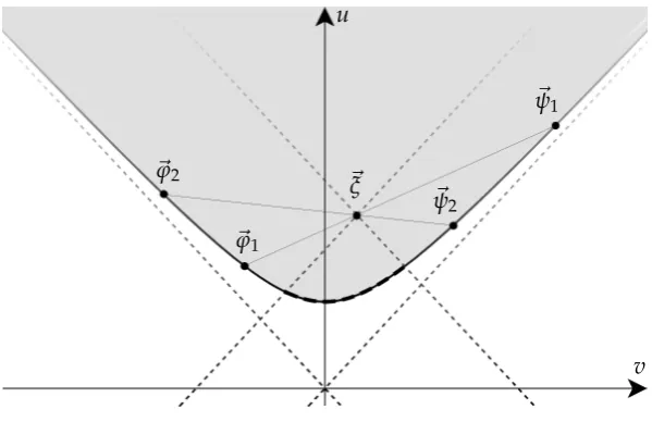
All moments arise as convex combinations of two pure states Consider a state|ξi giv-ing rise to the moment vector~ξ = (uξ,vξ,wξ)insidethe uncertainty region. It is possible to identify infinitely many pairs of Gaussian states on the boundary such that their mix-ture reproduces the given triple~ξ.

u

v ~_ξ

~

ψ1

~

ψ2 ~_ϕ1

~_ϕ2

Figure 1: Cross-section (w=0) of the uncertainty region (shaded) illustrating the convex-ity of its boundaryu2−v2−w2 =h¯2/4; convex combinations of moment triples located on the hyperboloid (associated with pure Gaussian states with minimal uncertainty) re-produce any given moment vector~ξ inside the uncertainty region (the points must be outside of the “back-ward light-cone” of the point~ξ, indicated by the dashed segment of the hyperbola).

“space-like” relative to~ξ and located on the hyperboloid, the pair determines a line in-tersecting the boundary in a unique point~ψ. Then, the desired point~ξ must lie on the line segment~ξ(t) = ~_ϕ+t(~_ψ−~_{ϕ), t ∈ [0, 1], connecting the points}~_ϕand~_{ψ; it will pass} through the point~ξif

t0 = uξ −uϕ uψ−uϕ ≡

vξ −vϕ

vψ−vϕ ∈[0, 1]. (86) When writing the line segment in the form~ξ(t) =t~ψ+ (1−t)~_{ϕ, it becomes obvious} that the reasoning valid in the space of moments extends to quantum states. In other words, the mixture

ˆ

ρt0 =t0Pψˆ + (1−t0)Pϕˆ (87)

of the rank-1 projectors ˆPψ =_|ψi hψ|and ˆPϕ =_|ϕi hϕ|onto Gaussian states on the bound-ary defines a mixed quantum state with the desired moment triple~ξ. Clearly, continu-ously many other convex combinations of pure states exist which lead to the same mo-ment triple.

with the fact that these Gaussian states are determined uniquely by their covariance ma-trixC.

5

Summary

We have presented a method to systematically determine lower bounds of uncertainty functionals, defined in terms of second moments of quantum systems with two or more continuous variables. In analogy to the one-dimensional case discussed in [13], we find that the states which extremize an uncertainty functional ofNdegrees of freedom must satisfy a (non-standard) eigenvalue equation which is quadratic in the 2N position and momentum operators. If the quadratic form associated with this operator is positive (or negative) definite, Williamson’s theorem ensures that it can be diagonalised by a sym-plectic transformation. In general, the matrix describing the quadratic form depends on the unknown state which suggests to solve it in a self-consistent way. The solutions of the resultingconsistency conditionsdetermine the set of states which minimise a given func-tional. We also introduced the N(2N+1)-dimensional uncertainty region for a system withNcontinuous variables. We show that this region is a convex subset of the space of second moments, and the points located on the boundary correspond to Gaussian states with minimal uncertainty.

Applying this method to specific functionals associated with quantum systems de-scribed by two continuous variables, we both re-derived existing uncertainty relations and previously unknown ones. We are not aware of other methods to obtain these in-equalities.

One of the new inequalities generalizes an existing inequality which is capable of de-tecting entanglement in states of bi-partite particle systems. This example hints at the possibility to systematically construct inequalities that can be used for entanglement tection: take an arbitrary number of EPR-type operators that pairwise commute, and de-fine a monotonically increasing function of their variances that is finite at the origin. Typ-ically, the lower bound given by the value of the functional at the origin will be achieved by anentangledstate, and it will be smaller than the value of the functional which it can take in any separable state. This bound can be obtained by solving the consistency condi-tions (39) for product states as described in Sec. 3.1. Clearly, a violation of the pure-state bound will detect the presence of an entangled state. The details of this construction will be left to a future publication.

Acknowledgements

References

[1] W. Heisenberg, Z. Phys.43, 172 (1927) [2] E. H. Kennard, Z. Phys.44, 326 (1927)

[3] H. Weyl,Gruppentheorie und Quantenmechanik(Hirzel, Leipzig, 1928) [English trans-lation, H. P. Robertson, The Theory of Groups and Quantum Mechanics (Dover, New York, 1931)]

[4] H. P. Robertson, Phys. Rev.34, 163 (1929)

[5] E. Schr ¨odinger, Sitzungsber. Preuss. Akad. Wiss. (Phys.-Math. Klasse)19, 296 (1930) [6] E. Arthurs and J. L. Kelly,Bell Syst. Tech. J.44, 725 (1965)

[7] P. Busch, P. Lahti and R. F. Werner, Phys. Rev. Lett.111, 160405 (2013) [8] M. Ozawa, Phys. Rev. A67, 042105 (2003)

[9] C. H. Bennett and G. Brassard, Proceedings of IEEE International Conference on Computers, Systems and Signal Processing, 175 (1984)

[10] L.-M. Duan, G. Giedke, J. I. Cirac, and P. Zoller, Phys. Rev. Lett.84, 2722 (2000) [11] R. Simon, Phys. Rev. Lett.84, 2726 (2000)

[12] R. Jackiw, J. Math. Phys.9, 339 (1968)

[13] S. Kechrimparis and S. Weigert, J. Phys. A (in print), arXiv:1509.02146

[14] D. S. Tasca, S. P. Walborn, P. H. S. Ribeiro, and F. Toscano, Physical Review A 78, 010304R (2008)

[15] F. Toscano, A. Saboia, A. T. Avelar, and S. P. Walborn, Phys. Rev. A 92, 052316 (2015) [16] E. C. Paul, D. S. Tasca, Ł. Rudnicki, S. P. Walborn:Detecting entanglement of continuous

variables with three mutually unbiased bases(preprint: arXiv:1604.07347 [quant-ph]) [17] P. Busch, T. P. Sch ¨onbeck and F. Schroeck Jr., J. Math. Phys.28, 2866 (1987)

[18] I. Bialynicki-Birula and Z. Bialynicka-Birula: Phys. Rev. Lett.108, 140401 (2012) [19] Ł. Rudnicki, Phys. Rev. A85, 022112 (2012)

[20] S. Weigert, Phys. Rev. A53, 2084-2088 (1996) [21] J. Williamson, Am. J. Math.58, 141 (1936)

[24] G. Adesso, S. Ragy, and A.R. Lee, Open Syst. Inf. Dyn.21, 1440001 (2014) [25] H. P. Robertson, Phys. Rev.46, 794 (1934)

[26] C. Weedbrook, S. Pirandola, R. Garcia-Patron, N. J. Cerf, T. C. Ralph, J. H. Shapiro, and S. Lloyd, Rev. Mod. Phys.84, 621 (2012)

[27] S. Boyd, L. Vanderberghe:Convex Optimization. (Cambridge University Press, Cam-bridge, 2004) p. 74