This is a repository copy of New use of global warming potentials to compare cumulative and short-lived climate pollutants.
White Rose Research Online URL for this paper: http://eprints.whiterose.ac.uk/108770/
Version: Accepted Version
Article:
Allen, MR, Fuglestvedt, JS, Shine, KP et al. (3 more authors) (2016) New use of global warming potentials to compare cumulative and short-lived climate pollutants. Nature Climate Change, 6. pp. 773-776. ISSN 1758-678X
https://doi.org/10.1038/nclimate2998
© 2016, Macmillan Publishers Limited. This is an author produced version of a paper published in Nature Climate Change. Uploaded in accordance with the publisher's self-archiving policy.
eprints@whiterose.ac.uk https://eprints.whiterose.ac.uk/ Reuse
Unless indicated otherwise, fulltext items are protected by copyright with all rights reserved. The copyright exception in section 29 of the Copyright, Designs and Patents Act 1988 allows the making of a single copy solely for the purpose of non-commercial research or private study within the limits of fair dealing. The publisher or other rights-holder may allow further reproduction and re-use of this version - refer to the White Rose Research Online record for this item. Where records identify the publisher as the copyright holder, users can verify any specific terms of use on the publisher’s website.
Takedown
If you consider content in White Rose Research Online to be in breach of UK law, please notify us by
A new use of Global Warming Potentials to relate the impacts of cumulative 1
and short-lived climate pollutants 2
3
Myles R. Allen, Jan S. Fuglestvedt, Keith P. Shine, Andy Reisinger, Raymond T. 4
Pierrehumbert & Piers M. Forster 5
6
Parties to the United Nations Framework Convention on Climate Change
7
(UNFCCC) have requested guidance on common greenhouse gas metrics in
8
accounting for Nationally Determined Contributions (NDCs) to emission
9
reductions1. Metric choice can affect the relative emphasis placed on
10
reductions of cumulative climate pollutants like carbon dioxide (CO2)
11
versus Short-Lived Climate Pollutants SLCPs including methane and
12
black carbon2,3,4,5,6. Here we show that the widely used 100-year Global
13
Warming Potential (GWP100) effectively measures relative impact of both
14
cumulative pollutants and SLCPs on realised warming 20-40 years after the
15
time of emission. If the overall goal of climate policy is to limit peak
16
warming, GWP100 therefore overstates the importance of current SLCP
17
emissions unless stringent and immediate reductions of all climate
18
pollutants result in temperatures nearing their peak soon after
mid-19
century7,8,9,10 which may be necessary to limit warming to well below 2
20
oC .1 The GWP100 can be used to approximately equate a one-off pulse
21
emission of a cumulative pollutant and an indefinitely sustained change in
22
the rate of emission of an SLCP11,12,13. The climate implications of
23
traditional CO2-equivalent targets are ambiguous unless contributions
24
from cumulative pollutants and SLCPs are specified separately.
25 26
Establishing policy priorities and market-based emission reduction mechanisms 27
involving different climate forcing agents all require some way of measuring 28
what one forcing agent is worth relative to another. The GWP100 metric has
29
been widely used for this purpose for over 20 years, notably within the UNFCCC 30
and its Kyoto Protocol. It represents the time-integrated climate forcing 31
perturbation to the Earth s balance between incoming and outgoing energy
32
due to a one-off pulse emission of one tonne of a greenhouse gas over the 100 33
years following its emission, relative to the corresponding impact of a one tonne 34
pulse emission of CO2. The notion of a temporary emission pulse is itself a rather
35
artificial construct: it could also be interpreted as the impact of a delay in 36
reducing the rate of emission of a greenhouse gas (see Methods). 37
38
This focus on climate forcing and 100-year time-horizon in GWP100 has no
39
particular justification either for climate impacts or for the policy goals of the 40
UNFCCC, which focus on limiting peak warming, independent of timescale. While 41
it could be argued that, given current rates of warming, the goal of the Paris 42
Agreement1to limit warming to well below oC focuses attention on mitigation
43
outcomes over the next few decades, this focus is only implicit and presupposes 44
that this goal will actually be met. Individual countries may also have goals to 45
limit climate impacts in the shorter term. These are acknowledged by the 46
UNFCCC, but not quantified in terms of, for example, a target maximum warming 47
rate. Metric choice is particularly important when comparing CO2 emissions with
SLCPs such as methane and black carbon aerosols. Black carbon has only 49
recently been introduced into a few intended NDCs14 but may become
50
increasingly prominent as some early estimates15 assign it a very high GWP100,
51
even though the net climatic impact of processes that generate black carbon 52
emissions remains uncertain16 and policy interventions to reduce black carbon
53
emissions are likely to impact6 other forms of pollution as well. Here we combine
54
the climatic impact of black carbon with that of reflective organic aerosols using 55
forcing estimates from ref. 16 (see Methods). 56
57
At least one party to the UNFCCC has argued17 that using the alternative Global
58
Temperature-change Potential (GTP) metric would be more consistent with the 59
UNFCCC goal of limiting future warming. )n its most widely used pulse variant2,
60
the GTP represents the impact of the emission of one tonne of a greenhouse gas 61
on global average surface temperatures at a specified point in time after 62
emission18, again relative to the corresponding impact of the emission of one
63
tonne of CO2. Figure 1 shows how both GTP and GWP values for SLCPs like
64
methane and black carbon depend strongly on the horizon. For long time-65
horizons, SLCP GTP values also depend on the response time of the climate 66
system, which is uncertain19,20. This latter uncertainty is a real feature of the
67
climate response that is not captured by GWP, and so is not itself a reason to 68
choose GWP over GTP. Other metrics and designs of multi-gas polices have been 69
proposed21,22, some of which can be shown to be approximately equivalent to
70
GWP or GTP23, but since only GWP and GTP have been discussed in the context of
71
the UNFCCC, we focus on these here. 72
73
For any time horizon longer than 10 years, values of the GTP are lower than 74
corresponding values of the GWP for SLCPs. The time-horizon has, however, a 75
different meaning between the two metrics: for GWP it represents the time over 76
which climate forcing is integrated, while for GTP it represents a future point in 77
time at which temperature change is measured. Hence there is no particular 78
reason to compare GWP and GTP values for the same time-horizon. Indeed, 79
figure 1 shows that the value of GWP100 is equal to the GTP with a time-horizon
80
of about 40 years in the case of methane, and 20-30 years in the case of black 81
carbon, given the climate system response-times used in ref. 16, for reasons 82
given in the Methods.24 Values of GWP and GTP for cumulative pollutants like
83
nitrous oxide (N2O) or sulphur hexafluoride (SF6) are determined primarily by
84
forcing efficiencies, not lifetimes, and are hence similar to each other and almost 85
constant over all these time-horizons.16 So for a wide range of both cumulative
86
and short-lived climate pollutants, GWP100 is very roughly equivalent to GTP20-40
87
when applied to an emission pulse, making it an approximate indicator of the 88
relative impact of a one-off pulse emission of a tonne of greenhouse gas or other 89
climate forcing agent on global temperatures 20-40 years after emission. The 90
inclusion of feedbacks between warming and the carbon cycle can substantially 91
increase GTP (and also, to a lesser degree, GWP) values, particularly on century 92
timescales25. Here we follow the traditional approach, used for the most
widely-93
quoted metric values in ref. 16, of including these feedbacks in modelling CO2 but
94
not other gases. 95
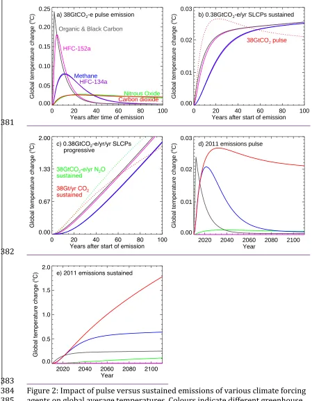
Figure 2, panel a, shows the impact on global average temperature of a pulse 97
emission of various climate pollutants, with the size of the pulse of each gas 98
being equivalent in terms of GWP100) to total anthropogenic CO2 emissions in
99
2011 (38 GtCO2): hence the pulse size is 38/GWP100 billion tonnes of each forcing
100
agent. SLCPs with high radiative efficiencies, like methane, black carbon and 101
some hydrofluorocarbons, have a more immediate impact on global 102
temperatures than notionally equivalent emissions of CO2, and less impact after
103
20-40 years. Hence, if the primary goal of climate policy is to limit peak warming, 104
then given the time likely to be required to reduce net global CO2 emissions to
105
zero to stabilise temperatures, the conventional use of GWP100 to compare pulse
106
emissions of CO2 and SLCPs is likely to overstate the importance of SLCPs for
107
peak warming until global CO2 emissions are falling.7,8
108 109
This is not an argument for delay in SLCP mitigation26 the benefits to human
110
health and agriculture alone would justify many proposed SLCP mitigation 111
measures4 but it is an argument for clarity in what immediate SLCP reductions
112
may achieve for global climate. The use of GWP100 to compare emission pulses
113
might still be appropriate to other policy goals, such as limiting the rate of 114
warming over the coming decades, although the impact of policies on warming 115
rates even over multi-decade timescales should always be considered in the 116
context of internal climate variability.27 Some contributions to the rate of
sea-117
level-rise also scale with integrated climate forcing.22
118 119
Simply adopting a different metric that assigns a lower weight to SLCP 120
emissions, such as GTP100, does not solve this overstatement problem, since any
121
metric that correctly reflects the impact of SLCPs on temperatures 100 years in 122
the future would understate their impact, relative to notionally equivalent 123
quantities of CO2, on all shorter timescales. Any choice of metric to compare
124
pulse emissions of cumulative and short-lived pollutants contains a choice of 125
time horizon16,18. It is, however, important for policy-makers to be clear about
126
the time-horizon they are focussing on. One problem with the GWP100 metric is
127
that warming may be interpreted colloquially to mean temperature rise by a 128
point in time , making the name misleading, because, in the case of SLCPs, 129
GWP100 actually delineates impact on temperatures in 20-40 years, not 100
130
years. 131
132
Figure 2b suggests an alternative way of using GWP100 to express equivalence
133
between cumulative and short-lived climate pollutants that is valid over a wider 134
range of time-scales, suggesting a way to use GWP100 to reconcile the emission
135
metrics literature2,3with the carbon budget approach9. The solid lines show
136
the impact on global temperatures of a sustained emission of 38 GtCO2
-137
equivalent (again computed using GWP100) of the short-lived climate pollutants
138
shown in 2a, but now starting abruptly in year 1 and distributed evenly over the 139
GWP time-horizon: hence a sustained emission rate of 38/(H×GWP100) billion
140
tonnes per year, where H=100 years. These cause temperatures to increase and 141
then approach stabilization after 20-40 years, depending on their lifetimes. The 142
dotted line shows the impact of a pulse emission of 38 GtCO2 in year one,
143
is not exact, but much better than in 2a, at least over timescales from 30 to 100 145
years. 146
The reason is simple: a pulse emission of an infinite-lifetime gas and a sudden 147
step change in the sustained rate of emission of a very-short-lifetime gas both 148
give a near-constant radiative forcing. If the total quantities emitted of both 149
gases over the 100-year GWP time-horizon is the same in terms of GWP100, then
150
the size of this radiative forcing, and hence the temperature response, will be 151
identical (see Methods for a more formal derivation). The solid and dotted lines 152
in figure 2b do not coincide exactly because CO2 is not simply an infinite-lifetime
153
gas, nor are the lifetimes of methane or black carbon completely negligible, 154
although the effective residence times of CO2 and these SLCPs are, crucially,
155
much longer and much shorter, respectively, than the 100-year GWP time 156
horizon. 157
A corollary is that a sustained step-change in the rate of emission of a cumulative 158
pollutant such as CO2 is approximately equivalent to a progressive linear increase
159
or decrease in the rate of emission of an SLCP. This is illustrated in figure 2c, 160
which compares the impact of a sustained emission of 38 Gt per year of CO2
161
emissions (red dotted line) with SLCP emissions increasing from zero at a rate of 162
0.38 GtCO2-e per year per year (solid lines). Again, although the correspondence
163
is not exact, it is much better than the nominally equivalent emission pulses in 164
2a. The green dotted line shows that sustained emissions of cumulative 165
pollutants (N2O and CO2) have similar impacts on these timescales. Finally, a
166
progressive change in the rate of emission of CO2, necessary to reach net zero10
167
CO2 emissions to stabilise temperatures, could only be equated to an accelerating
168
change in SLCP emissions. This last equivalence is somewhat moot because 169
attempting to match the rates of reduction of CO2 emissions28 required to limit
170
warming to 2 oC would result in SLCP emissions soon having to be reduced
171
below zero. In summary, therefore, a pulse (or sustained) emission of a 172
cumulative pollutant may be approximately equivalent to a sustained (or 173
progressively increasing) change in the rate of emission of an SLCP, but there is 174
no substitute for a progressive reduction in the rate of emission a cumulative 175
pollutant such as CO2, which remains the sine qua non of climate stabilisation.
176 177
This correspondence between pulse emissions of cumulative pollutants and 178
sustained emissions of short-lived pollutants (or the benefits of corresponding 179
emissions reductions) has been noted before7,8,11,12,13, but previous studies
180
suggested that a new metric of sustained emission reductions would be required 181
to relate them. Figure 2b suggests that the familiar GWP100 might still be
182
adequate for this purpose, provided it is used to relate sustained reductions in 183
emission rates of SLCPs (agents with lifetimes much shorter than the GWP time-184
horizon) with temporarily avoided emissions of cumulative climate pollutants 185
(any with lifetimes substantially longer than the GWP time-horizon). 186
187
There are obvious challenges to incorporating this second use of GWP100 into the
188
UNFCCC process. The Kyoto Protocol and most emissions trading schemes are 189
predicated on emissions accounting over fixed commitment periods. Although 190
commitment to a permanent reduction in an SLCP emission rate with actual 192
avoided emissions of a cumulative pollutant within a commitment period would 193
be a significant policy innovation. Nevertheless, this approximate equivalence 194
may be useful in setting national or corporate climate policy priorities, 195
particularly where decisions involve capital investments committing future 196
emissions13.
197 198
This second use of GWP100 is also relevant to the long-term goal in the Paris
199
Agreement to achieve a balance between anthropogenic emissions by sources
200
and removals by sinks in order to hold the increase in the global average 201
temperature to well below 2°C above pre-industrial levels. Peak warming scales 202
approximately with cumulative CO2 and N2O emissions (expressed as GtCO2-e
203
using GWP100) between now and the time of peak warming plus the sustained
204
rate of emission of SLCPs (expressed in GtCO2-e/H per year, with H=100 years if
205
GWP100 is used to define GtCO2-e) in the decades immediately prior to peak
206
warming. So a sustained emission rate of 0.01 tonnes per year of methane has 207
the same impact on peak warming as a pulse of 28 tonnes of CO2 released at any
208
time between now and when temperatures peak, GWP100 of methane being 28.
209
As NDCs are updated, it would be useful for countries to clarify how they 210
propose to balance (individually or collectively) cumulative emissions of CO2 and
211
N2O as these are reduced to zero or below with future emission rates of SLCPs.
212 213
Figure 2d shows the impact on global temperatures of actual 2011 emissions of 214
various climate pollutants, considered as a one-year emission pulse.16 Methane
215
and black carbon emissions in 2011 have a comparable or even larger impact on 216
global temperatures over the next couple of decades than 2011 CO2 emissions,
217
but their impact rapidly decays, while the impact of current CO2 emissions
218
persists throughout the 21st century and for many centuries beyond.
219 220
Figure 2e shows the impact of 2011 emissions of various climate pollutants, 221
assuming these emissions are maintained at the same level for the next 100 222
years. The warming impact of the cumulative pollutants, CO2 and nitrous oxide,
223
increases steadily as long as these emissions persist, while sustained emissions 224
of methane and organic and black carbon aerosols cause temperatures to warm 225
rapidly at first and then stabilize. A permanent reduction of 50-75% in these 226
SLCPs could reduce global temperatures by over 0.5oC by mid-century4,
227
comparable to the impact on these timescales of similar-magnitude reductions of 228
CO2 emissions and, it has been argued, at much lower cost4,5,29. Stabilising global
229
temperatures, however, requires net emissions of cumulative pollutants, 230
predominantly CO2, to be reduced to zero.
231 232
The notion of CO2-equivalent pulse emissions of cumulative and short-lived
233
climate pollutants will always be ambiguous because they act to warm the 234
climate system in fundamentally different ways. To date, this ambiguity may 235
have had only a limited impact, not least because emission reductions have so far 236
been relatively unambitious. As countries with relatively large agricultural 237
emissions of methane and significant black carbon emissions begin to quantify 238
increases consistent with the collective goal of limiting warming to well below 240
2°C, this situation may change21,30.
241 242
For their long-term climate implications to be clear, policies and Nationally 243
Determined Contributions need to recognise these differences. GWP100 can be
244
used in the traditional way, comparing pulse emissions of different greenhouse 245
gases, to specify how mitigation of both short-lived and cumulative climate 246
pollutants may reduce the rate and magnitude of climate change over the next 247
20-40 years, but only over that time. To achieve a balance between sources and 248
sinks of greenhouse gases in the very long term, net emissions of cumulative 249
pollutants such as CO2 need to be reduced to zero, while emissions of SLCPs
250
simply need to be stabilised. GWP100 can again be used, but in the second way
251
identified here, to relate cumulative (positive and negative) emissions of CO2
252
until these reach zero with future emission rates of SLCPs, particularly around 253
the time of peak warming. Some NDCs are already providing a breakdown in 254
terms of cumulative and short-lived climate pollutants, or differential policy 255
instruments for different forcing agents30 and different timescales, all of which is
256
needed for their climatic implications to be clear. The Paris Agreement proposes 257
that Parties will report emissions and removals using common metrics, but a 258
generic CO2-equivalent emission reduction target by a given year, defined in
259
terms of GWP100 and containing a substantial element of SLCP mitigation,
260
represents an ambiguous commitment to future climate. The conventional use of 261
GWP100 to compare pulse emissions of all gases is an effective metric to limit
262
peak warming if and only if emissions of all climate pollutants, most notably CO2,
263
are being reduced such that temperatures are expected to stabilise within the 264
next 20-40 years. This expected time to peak warming will only become clear 265
when CO2 emissions are falling fast enough to observe the response. Until such a
266
clear end-point is in sight, only a permanent change in the rate of emission of an 267
SLCP can be said to have a comparable impact on future temperatures as a one-268
off pulse emission of CO2, N2O or other cumulative pollutant.
269 270
Acknowledgements: MRA was supported by the Oxford Martin Programme on 271
Resource Stewardship. MRA and KPS received support from the UK Department 272
of Energy and Climate Change under contract no. TRN/307/11/2011; JSF from 273
the Norwegian Research Council, project no. 235548; RTP from the Kung Carl 274
XVI Gustaf 50-års fond; PMdF from the UK Natural Environment Research 275
Council grant no. NE/N006038/1. The authors would like to thank three very 276
helpful anonymous reviewers who considerably clarified this work and 277
numerous colleagues, particularly among IPCC authors, for discussions of 278
metrics over recent years. 279
Methods
280
The equality of GWP100 and GTP20-40 follows from the idealised expressions for 281
GWP and GTP for a pulse emission given in ref. 2 (equations A1 and 3 in ref. 2, 282
expressed as relative GWP and GTP respectively, and with decay-times replaced 283
by decay rates): 284
GWP (1)
285
GTP (2) 287
where is the instantaneous forcing per unit emission and the concentration 288
decay rate for a greenhouse gas, with and the corresponding parameters 289
for a reference gas, is a typical thermal adjustment rate of the ocean mixed 290
layer in response to forcing, and and are the GWP and GTP time-horizons. 291
For a very short-lived greenhouse gas and very long-lived reference gas such 292
that , , , and , the terms in
293
parentheses in the numerator and denominator of equations (1) and (2) are 294
approximately unity, , and respectively. Hence, using
295
and , we have
296
GWP and GTP
297
so GWP equals GTP if ln , or 21 years if years and
298
years , as in ref. 16. Hence in the limit of a very short-lived gas and 299
infinitely persistent reference gas, the GTP for a pulse emission evaluated at 21 300
years will be equal to the GWP100. The expression becomes more complicated if
301
as is the case of methane, but this limiting case serves to show that the 302
equality of GWP100 and GTP20-40 arises primarily from the thermal adjustment
303
time of the climate system. 304
305
The approximate equivalence of the temperature response to a one-tonne 306
transitory pulse emission of a cumulative pollutant to sustained step-change in 307
the rate of emission of an SLCP by 1/(H×GWPH) tonnes per year, where H is the
308
GWP time horizon, follows from the cumulative impact of CO2 emissions on
309
global temperatures. This means that the temperature response at a time H after 310
a unit pulse emission of CO2 (AGTPP(CO2) in ref. 2), multiplied by H, is
311
approximately equal to the response after time H to a one-unit-per-year 312
sustained emission of CO2 (AGTPS(CO2)), provided H is shorter than the effective
313
atmospheric residence time of CO2, which is of order millennia. This is consistent
314
with the concept of the trillionth tonne that it is the cumulative amount of 315
CO2 that is emitted, rather than when it is emitted, that matters most for future
316
climate9. Ref. 2 also notes that the ratio AGTPS(x)/AGTPS(CO2) is approximately
317
equal to GWP (x) for time horizons H much longer than the lifetime of an agent x. 318
Hence: 319
320
AGTPS GWP AGTPS CO GWP AGTPP CO (3)
321 322
provided H is shorter than the effective residence time of CO2 and longer than
323
the lifetime of the agent x, as is the case when H=100 years and x is an SLCP. 324
325
The interpretation of an avoided emission pulse , although central to most 326
emission trading schemes, may be ambiguous in the context of many mitigation 327
decisions, which may involve policies resulting in permanent changes in 328
emission rates. Another way of expressing this notion of an avoided pulse is in 329
terms of the impact of delay in reducing emissions of cumulative pollutants: a 330
five year delay in implementing a one-tonne-per-year reduction of CO2 emissions
331
tonnes-per-year of methane (GWP100 of methane
333
being 28). This would only compensate for the direct impact of the delay in CO2
334
emission reductions, not for additional committed future CO2 emissions that
335
might also result from that delay.28
336 337
Treatment of Black Carbon emissions: Focusing solely on absorbing aerosols 338
gives a high estimated radiative efficiency impact on the global energy budget
339
per unit change in atmospheric concentration) for black carbon, a strong positive 340
global climate forcing15 (1.1 W m-2 in 2011) and a GWP100 of 910. This figure has
341
been argued16 to be too high, and the actual radiative impact of individual black
342
carbon emissions depends strongly on the circumstances (location, season and 343
weather conditions) at the time of emission. Many processes that generate black 344
carbon also generate reflective organic aerosols, which have a cooling effect on 345
global climate. Although ratios vary considerably across sources, policy 346
interventions to limit black carbon emissions are likely also to affect these other 347
aerosols, so it might be more relevant to consider their combined impact: the 348
current best estimate16 net global radiative forcing of organic and black carbon
349
aerosols in 2011 was 0.35 W m-2, giving a combined GWP100 of 290, used in the
350
figures. Combined emissions of organic and black carbon aerosols are inferred 351
from this GWP100 value assuming all radiative forcing resulting from these
352
emissions is concentrated in the first year (i.e. a lifetime much shorter than one 353
year). This is only one estimate of a very uncertain quantity: when both 354
reflection and absorption are taken into account, including interactions between 355
aerosols and clouds and surface albedo, even the sign of the net radiative impact 356
of the processes that generate black carbon aerosols remains uncertain. 357
358
Modelling details: Figure 1: GWP values calculated using current IPCC methane 359
and CO2 impulse response functions without carbon cycle feedbacks.16 Radiative
360
forcing (RF) of a pulse emission of organic and black carbon aerosols 361
concentrated in year 1, scaled to give a net GWP100 of 290, consistent with ratio
362
of 2011 RF values given in refs. 15 and 16. GTP values calculated using the 363
standard IPCC AR5 thermal response model (solid blue lines) with coefficients 364
adjusted (dotted blue lines) to give Realised Warming Fractions24 (ratio of
365
Transient Climate Response, TCR, to Equilibrium Climate Sensitivity, ECS) of 0.35 366
and 0.85, spanning the range of uncertainty around the best-estimate value of 367
0.56. Figure 2: As figure 1 with radiative efficiencies and lifetimes provided in 368
Table A.8.1 of ref. 16 and representative mid-range values of TCR=1.5oC and
369
ECS=2.7oC.
Figures
372 373
374
Figure 1: Values of Global Warming Potential (red) and Global Temperature-375
change Potential (blue) for methane and combined organic and black carbon as a 376
function of time-horizon. Solid lines show metrics calculated using current IPCC 377
response functions16; dotted blue lines show impact of varying the climate
378
response time (see Methods). Black dotted lines show the value of GWP100.
379 380
0 20 40 60 80 100
Time-horizon 1
10 100
a) Methane metric value
GTP
GWP
0 20 40 60 80 100
Time-horizon 1
10 100 1000 10000
b) Organic & black carbon metric value
GTP
381
382
[image:11.595.52.501.76.654.2]383
Figure 2: Impact of pulse versus sustained emissions of various climate forcing 384
agents on global average temperatures. Colours indicate different greenhouse 385
gases, with grey lines indicating combined impact of reflective organic and black 386
carbon aerosols (see Methods) a) Warming caused by a pulse emission in 2011 387
with each pulse size being nominally equivalent, using GWP100, to 2011
388
emissions of CO2. b) Solid lines: impact of sustained emissions of SLCPs at a rate
389
equivalent to 2011 emissions of CO2 spread over the 100-year GWP100 time
390
horizon. Dotted line shows impact of pulse emission of CO2 reproduced from (a).
391
c) Solid lines: impact of SLCP emissions progressively increasing from zero at 392
0 20 40 60 80 100
Years after time of emission 0.00
0.05 0.10 0.15 0.20 0.25
G
lo
b
a
l
te
m
p
e
ra
tu
re
c
h
a
n
g
e
(
o C
) a) 38GtCO2-e pulse emission
Carbon dioxide
Methane
Nitrous Oxide
HFC-134a HFC-152a
Organic & Black Carbon
0 20 40 60 80 100
Years after start of emission 0.00
0.01 0.02 0.03
G
lo
b
a
l
te
m
p
e
ra
tu
re
c
h
a
n
g
e
(
o C
) b) 0.38GtCO2-e/yr SLCPs sustained
38GtCO2 pulse
2020 2040 2060 2080 2100 Year
0.00 0.01 0.02 0.03
G
lo
b
a
l
te
m
p
e
ra
tu
re
c
h
a
n
g
e
(
o C
0.38 GtCO2-e yr-2. Dotted lines: impact of sustained emissions of CO2 and N2O at
393
38 GtCO2 (or equivalent) per year. d) Impact of actual 2011 emissions of each
394
climate forcing agent expressed as a pulse. e) Impact of emissions sustained 395
indefinitely at 2011 rates. 396
397
References:
398
1 United Nations Framework Convention on Climate Change (2015): Adoption of
the Paris Agreement, FCCC/CP/2015/L.9/Rev.1.
2 Shine, K., Fuglestvedt, J., Hailemariam, K. & Stuber, N. (2005): Alternatives to
the global warming potential for comparing climate impacts of emissions of greenhouse gases, Clim. Change, 68, 281 302.
3 Fuglestvedt J.S., et al (2010): Assessment of transport impacts on climate and
ozone: metrics Atmospheric Environment 44:4648-4677
4 Shindell, D. et al (2012): Simultaneously mitigating near-term climate change
and improving human health and food security, Science,335, 183 189.
5 Victor, D. G., Kennel, C. F. & Ramanathan, V (2012): The climate threat we can
beat. Foreign Aff. 91, 112 114 & http://new.ccacoalition.org/en
6 Rogelj, J., et al (2014): Disentangling the effects of CO2 and short-lived climate
forcer mitigation, Proc. Nat. Acad. Sci., 111, 16325-16330.
7 Bowerman, N. H. A. et al (2013): The role of short-lived climate pollutants in meeting temperature goals, Nature Climate Change, 3, 1021 1024.
8 Pierrehumbert, R. T. (2014): Short-lived climate pollution, Ann. Rev. Earth &
Planetary Sciences,42, 341-379.
9 Allen, M. R. et al (2009): Warming caused by cumulative carbon emissions
towards the trillionth tonne, Nature,458, 1163 1166.
10 Matthews, H. D. and Caldeira, K. (2008): Stabilizing climate requires near-zero
emissions, Geophys. Res. Lett.35 (4), GL032388.
11 Smith, S. M. et al (2012): Equivalence of greenhouse-gas emissions for peak
temperature limits, Nature Climate Change, 2: 535-538.
12 Lauder, A. R. et al (2013): Offsetting methane emissions An alternative to
emission equivalence metrics, Int. J. Greenhouse Gas Control, 12, 419-429.
13 Alvarez, R. A., et al (2012): Greater focus needed on methane leakage from
natural gas infrastructure, Proc. Nat. Acad. Sci., 109, 6435-6440
14 Government of Ecuador (2015): Intended Nationally Determined Contribution,
Submission to the UNFCCC, http://www4.unfccc.int/submissions/INDC/
15 Bond, T. C. et al. (2013), Bounding the role of black carbon in the climate
system: A scientific assessment, J. Geophys. Res. Atmos., 118, no. 11, 5380-5552.
16 Myhre, G. et al (2013): Anthropogenic and natural radiative forcing. Chapter 8
of Stocker, T.F., Qin, D. et al, Climate Change 2013: The Physical Science Basis, Cambridge University Press, Cambridge and New York, NY.
17 Government of Brazil (2015): Intended Nationally Determined Contribution,
Submission to the UNFCCC, http://www4.unfccc.int/submissions/INDC/
18 Shine K. P. et al, (2007): Comparing the climatic effects of emissions of short-
19 D. J. L. Olivié and G. P. Peters (2013): Variation in emission metrics due to
variation in CO2 and temperature impulse response functions, Earth System
Dynamics, 4, 267-286
20 Reisinger, A., et al (2011): Future changes in Global Warming Potentials under
Representative Concentration Pathways, Environ. Res. Lett.6, 024020
21 Daniel, J. S. et al (2012): Limitations of single-basket trading: lessons from the
Montreal Protocol for climate policy, Clim. Change,111, 241 248.
22 Johansson D (2012): Economics- and physical-based metrics for comparing
greenhouse gases, Clim. Change110:123-141.
23Peters, G., B. Aamaas, T. Berntsen, and J. Fuglestvedt (2011): The integrated global temperature change potential (iGTP) and relationships between emission metrics. Environ. Res. Lett., 6, 044021.
24 Millar, R. J. et al, (2015): Model structure in observational constraints on the
transient climate response, Clim. Change, 131, 199-211
25Gillett, N. P. and H. D. Matthews (2010) Accounting for carbon cycle feedbacks in a comparison of the global warming effects of different greenhouse gases,
Environ. Res. Lett., 5, 034011.
26 Schmale, J. et al (2014): Air pollution: Clean up our skies, Nature, 515,
335-337.
27 Deser, C. et al. (2010): Uncertainty in climate change projections: the role of
internal variability, Clim. Dyn.38, 527-546.
28 Allen, M. R. & Stocker, T. F. (2013): Impact of delay in reducing carbon dioxide
emissions, Nature Climate Change, 4, 23 26.
29 Huntingford, C. et al, (2015): The implications of carbon dioxide and methane
exchange for the heavy mitigation RCP2.6 scenario under two metrics, Env. Sci. &
Policy, 51, 77-87
30 Government of New Zealand (2015): Intended Nationally Determined