Supercomputer Emulation For Evaluating Scheduling Algorithms

(1)

Supercomputer Emulation For

Evaluating Scheduling Algorithms

Claudio Barberato

A thesis submitted for the degree of

Master of Philosophy

The Australian National University

(2)

c

(3)

Except where otherwise indicated, this thesis is my own original work.

(4)

(5)

(6)

(7)

Acknowledgments

I would like to thank my supervisory panel, Dr Eric McCreath, Associate Professor Peter Strazdins and Dr Muhammad Atif for their indispensable guidance, without which the completion of this thesis would not be possible.

(8)

(9)

Abstract

Scheduling algorithms have a significant impact on the optimal utilization of HPC facilities, yet the vast majority of the research in this area is done using simulations. In working with simulations, a great deal of factors that affect a real scheduler, such as its scheduling processing time, communication latencies and the scheduler intrin-sic implementation complexity are not considered. As a result, despite theoretical improvements reported in several articles, practically no new algorithms proposed have been implemented in real schedulers, with HPC facilities still using the basic first-come-first-served (FCFS) with Backfill policy scheduling algorithm.

A better approach could be, therefore, the use of real schedulers in an emulation environment to evaluate new algorithms.

This thesis investigates two related challenges in emulations: computational cost and faithfulness of the results to real scheduling environments.

It finds that the sampling, shrinking and shuffling of a trace must be done carefully to keep the classical metrics invariant or linear variant in relation to size and times of the original workload. This is accomplished by the careful control of the submission period and the consideration of drifts in the submission period and trace duration. This methodology can help researchers to better evaluate their scheduling algorithms and help HPC administrators to optimize the parameters of production schedulers. In order to assess the proposed methodology, we evaluated both the FCFS with Backfill and Suspend/Resume scheduling algorithms. The results strongly suggest that Suspend/Resume leads to a better utilization of a supercomputer when high priorities are given to big jobs.

(10)

(11)

List of Figures

3.1 A normal Slurm based cluster configuration: One slurmctld daemon

running in the Head Node (HN) and one slurmddaemon running in

each Computing Node (CN). . . 16

3.2 Cluster emulation using Slurm Front End and Multiple slurmds

fea-tures. (a) A single slurmctld and single slurmd can run in the Head

Node (HN), or in a desktop, if Slurm is compiled with the Front End option. In this case, the emulated nodes will be set up in the Slurm configuration file but all job management will be accomplished by the

single slurmd. (b) Additionally to the Front End option we can also

run multiples slurmds in a single computing node with the Multiple

Slurmd option. As in (a) the emulated nodes will be also set up in the configuration file, but the management of all the jobs will be shared

between the severalslurmds. . . 17

3.3 A cluster emulation with aslurmctldin the head node (HN) and

multi-plesslurmdsin each computing node (CN). . . 18

4.1 Raijin’s job size distribution (Y axis is logarithmic) . . . 26

4.2 Raijin’s job submission time distribution. . . 26

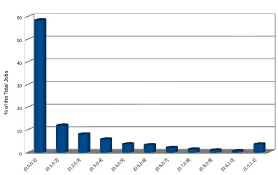
4.3 Users’ accuracy for their job runtime estimates. X-axis contains the

intervals for the ratio between the actual runtime and estimated run-time. Y-axis shows the percentage of these jobs in relation to the total number of jobs in the workload. For instance, all jobs with a runtime estimate equal or bigger than 10 times the actual runtime are grouped in the (0.0,0.1] interval which represents 58% of all submitted jobs. . . . 28

4.4 Waiting time values for a workload with the submission order shuffled

10 times. Each new workload gives rise to three more workloads. The first workload has all jobs with the same priority, the second contains

20% of the jobs randomly assigned with high priority (rand), and, in

the third workload, high priorities are assigned only to jobs asking for

700 or more CPUs (size). Backfill is applied to all these workloads and

the resulting Waiting Times are labeledbf, bf (rand), andbf (size).

Sus-pend/Resume is applied only to the workloads with different priorities

and the resulting Waiting Times are labeledsr (rand)andsr (size). . . 33

4.5 Response Time values for the same set up shown in Figure 4.4. . . 33

4.6 Slowdown values for the same set up shown in Figure 4.4. . . 34

4.7 Weighted Slowdown values for the same set up shown in Figure 4.4. . 34

(14)

xiv LIST OF FIGURES

4.8 Utilization values for the same set up shown in Figure 4.4. . . 35

4.9 Raijin’s job daily submission distribution for the 4 most popular job

sizes normalized by their average. 1 core jobs displayed an average of 10,028 jobs/day, 2 core jobs 2,220 jobs/day, 8 core jobs 1,423 jobs/day, and 16 core jobs 1,715 jobs/day. . . 37 4.10 Comparison between original and sampled workload (scaled) job size

distribution (Y axis is logarithmic). The scale factor (147.2) is the num-ber of jobs in the original workload (4,417,018) divided by the numnum-ber of jobs in the sampled workload (30,000). . . 37 4.11 Classical metrics for 17 sampled workloads scheduled with Backfill. . . 40 4.12 Preliminary results for time shrinking. . . 41 4.13 Classical Metrics behaviour using wall clock submission time. . . 42 4.14 Classical Metrics behaviour using wall clock and drift corrections for a

30,000 jobs processed in a 57600-CPU cluster. . . 44

5.1 Cluster utilization affected by the submission of 31 big jobs. Only the

submission (red line) of a high priority 20,000-CPU job for Backfill is shown. The drop in the utilization after this submission is related to the time necessary to reserve enough CPUs to start (yellow line) this job. 49

5.2 Cluster utilization affected by the submission high priority jobs for

Suspend/Resume scheduling algorithm. The drops in the utilization coincides with the submission of big-high priority jobs. For comparison with Backfill the submission, the start and end of the 20,000-CPU job is also shown. The start instance (yellow line) coincides with the start (red line) since the Suspend/Resume algorithm starts a high priority job as soon as it is submitted. . . 50

5.3 Cluster utilization, high priority jobs and suspended jobs. This graph

shows that the implementation of Slurm for Suspend/Resume is sus-pending more low priority jobs than necessary to run a higher priority job. . . 50

5.4 Cluster utilization for Backfill for a new workload a utilising the Linear

Plugin. All jobs in this workload ask now for at least 16 CPUs (A whole node). The overall behaviour is still the same as presented in Figure 5.1 51

5.5 Cluster utilization, high priority jobs and suspended jobs. This graph

shows the Linear plugin suspends only the necessary number of lower priority jobs to run higher priority jobs, which results in a high cluster utilization. . . 51

A.1 Sleep program demonstration using abashscript. . . 57

A.2 Demonstration that thesleepprogram is not affect by suspensions. . . . 58

(15)

List of Tables

2.1 Scheduling parameters. . . 8

3.1 Cluster parameters. . . 19

3.2 Software Platforms . . . 24

4.1 Job size and its percentage of total jobs . . . 25

4.2 Job size and its percentage of total Service Units (S.U.) . . . 27

4.3 Stability of the classical metrics over the course of 5 consecutive runs. The columns are Waiting Time (WT), Response Time (RT), Slowdown (SD), Weighted Slowdown (WS) and Utilization (UT). The last 4 rows are the Average (AVE), Standard Deviation (SSD), Relative Standard Deviation (RSD) and the Confidence Interval with a level of Confidence of 95% (C95) . This notation will be repeated in the following tables. . . 28

4.4 Classical Metrics for a workload shuffled 10 times. All jobs had the same priority and they were scheduled with Backfill. . . 30

4.5 Classical Metrics for the same workloads and algorithm (Backfill) de-scribed in Table 4.4. The columns labeledRandom Prioritieshad 20% of their jobs randomly assigned with high priority and the remaining jobs with low priority. The columns labeled Size Based Priorities had only jobs requesting 700 or more CPUs assigned with high priority. . . 31

4.6 Classical Metrics for the same configuration as in Table 4.5. The scheduling algorithm used was suspend/resume. . . 31

4.7 Classical Metrics for the workload described in Section 4.2.3 shuffled 6 times. The resulting trace was obtained using backfill as the scheduling algorithm. All jobs had the same priority. . . 32

4.8 Classical metrics for 10 different workloads with a sampling ratio of 147.2, but with different offsets using Backfill. . . 39

4.9 Trace with 10 equal jobs with runtime of 60 seconds being submitted at regular intervals of 60 seconds. The time delay between the ending of a job and the starting of the next induces a drift around 0.1 second per submission in the start time of each job. The accumulated effect of this drift by the 10thsubmission is around 1 second. . . 43

5.1 Backfill and Suspend/Resume comparison using Linear plugin. The standard deviation for each metric (5 runs) is shown in parentheses. . . 49

(16)

(17)

Chapter1

Introduction

1 .

1 Thesis Statement

The emulation of a supercomputer environment is a more powerful alternative for evaluating scheduling algorithms than simulation because the first automatically takes into account the scheduling processing time, communication latencies, multi programming and fragmentation. Emulation is viable if the processing time of a workload can be reduced by means of sampling and time shrinking.

1 .

2 Problem Statement

A supercomputer is a high-level performance computer composed of thousands of processing units or cores organized into nodes that are connected by a state-of-art network. Supercomputers are specially designed to carry out the computation of large problems called jobs. These big problems require multiple processing units for their timely completion.

A scheduler is a program that decides when and where a job is going to run. This problem grows in complexity when the number of cores requested by incoming jobs exceeds the capacity of the supercomputer [Feitelson and Rudolph, 1995; Feitelson et al., 1997; Feitelson, 1997; Feitelson et al., 2005].

A good scheduler will optimize the use of the resources, e.g., processing units, resulting in a better return for the High Performance Computing (HPC) investment. This makes research into scheduling algorithms a hot topic in computer science. The problem is complex because it requires dealing with various, sometimes conflicting, requirements such as the number of cores, total of requested and used memory, priorities among many others [Lifka, 1995].

The usual approach in developing scheduling algorithms involves the use of simu-lators [Schwiegelshohn and Yahyapour, 1998]. Traditionally, simusimu-lators are relatively simple programs developed by researchers to test their hypotheses. A simulator usually reads a file with the workload of a supercomputer facility to sort the jobs according to established and newly proposed algorithms. The basic information con-tained in these workloads is the arrival time, the number of requested nodes and the estimated and run time of each job. The outcome of these simulations may contain

(18)

2 Introduction

information about when a job was submitted, started, finished and the used nodes. This information can be used to evaluate scheduling metrics like average waiting time, average response time and overall system throughput. These metric values form, then, the basis for performance comparisons between scheduling algorithms.

However, despite theoretical improvements reported in several articles [Yuan et al., 2014; Niu et al., 2012; Niemi and Hameri, 2012], practically no new proposed algorithms have been implemented in real schedulers with most HPC facilities still using the basic first-come-first-served (FCFS) with backfill policy scheduling algo-rithm [Schwiegelshohn and Yahyapour, 1998].

In the present work, instead of disregarding all aspects related to the resource management, the chosen approach was to use a real system in an emulation environ-ment to overcome the limitations of the simulators. The emulation environenviron-ment was composed of a cluster of virtual machines managed by a real scheduler and running dummy jobs which were responsive to suspend and continue signals.

1 .

3 Scope

There are several aspects affecting the evaluation of job scheduling in supercom-puters, such as the scheduling processing time, workload structure, communication latencies, communication within a job, memory availability, interactive jobs, multi programming level inside a processing unit, fragmentation, warm up and cool-down periods. A great deal of these factors are usually not considered when working with simulations.

In the present work, due to the fact that emulations are closer to reality, most of these aspects are automatically considered, like scheduling processing time, commu-nication latencies, multi programming and fragmentation. Additionally, the warm up and cool-down periods are also taken into account in our experiments.

However, this thesis does not investigate the workload structure, communications within a job, memory availability and interactive jobs.

1 .

4 Contributions

This thesis uncovers the related challenges to perform timely emulations which results can be safely extrapolate to the original workload. The main contributions of this thesis are:

• The introduction of a simple, but effective, framework to support the evaluation

of scheduling algorithms.

• The development of an efficient program, sigsleep, that plays the role of an

(19)

§1.5 Thesis Outline 3

which allows the direct evaluation of the performance metrics. The source code of this program is presented in Appendix C.

• The development of a submission script that reads a workload and precisely

submitssigsleepjobs to the scheduler.

• The development of a program to evaluate the classical metrics based on the

information logged bysigsleep.

• The study of four artefacts, concurrency, submission order, sampling and time

shrinking that affect the scheduling process and how to overcome their effects on the evaluation of the scheduling metrics.

• The use of the developed framework to evaluate the implementation of two

popular scheduling algorithms, Backfill and Suspend/Resume, in Slurm. We found that Suspend/Resume shows a better performance in comparison to Backfill only when big jobs are presented in the workload.

• The uncovering of a lack of optimization in the Suspend/Resume

implementa-tion in Slurm when used in conjuncimplementa-tion with the Consumable Resources plugin.

1 .

5 Thesis Outline

This thesis has 6 chapters. Chapter 1 states the problems this thesis will address, defines its scope and outlines its contributions.

Chapter 2 introduces the most relevant concepts related to supercomputers, clus-ters, cloud computing and classical scheduling metrics. It also presents a literature review of the current research on scheduling algorithms using both simulation and emulation.

Chapter 3 explains how the environment used in our experiments was set up. It also describes the hardware and software platforms used to create this environ-ment, along with the algorithms and programs developed to evaluate scheduling algorithms.

Chapter 4 discusses the experimental methodology applied in the experiments performed in this work. This chapter also introduces the key concepts of the classical metrics artefacts.

The results of the application of the aforementioned methodology for the eval-uation of two scheduling algorithms by means of the emulation are presented in Chapter 5.

(20)

(21)

Chapter2

Background and Related Work

This chapter provides the background knowledge required to develop this thesis. It also contains a comprehensive literature review about simulation, emulation, schedul-ing algorithms development and the strategies for their evaluation. This chapter starts by introducing the basic concepts related to this work in Sections 2.1 and 2.2, and then progresses to explaining supercomputer scheduling in Section 2.3. Section 2.4 gives a brief introduction to classical scheduling metrics while Section 2.5 defines and compares simulation and emulation. Sections 2.6 and 2.7 review and discuss previous works on the usage of simulation and emulation to evaluate scheduling algorithms.

2 .

1 Supercomputer, Computer Cluster and Cloud Computing

A supercomputer is a high-level performance computer composed of thousands of processing units designed for HPC. A computer cluster is a set of processing units, called nodes, connected by a network and used as a single computer. The use of high-speed networks and powerful microprocessors associated with computer clusters can turn them into very cost effective supercomputers [Baker and Buyya, 1999].

Cloud computing is a way of sharing computational resources over the Internet. It is implemented by adding a layer of hardware virtualization called hypervisor that, among many other functionalities, creates, destroys and runs virtual machines (VM). Cloud computing is, therefore, a flexible and cost-effective computational environ-ment where computational resources can be allocated on demand. Nevertheless, this flexibility may come at the expense of a deteriorated performance due to the extra work demanded by the hypervisor.

However, due to recent developments in hardware and software, cloud computing is being increasingly considered as an alternative platform for HPC [Atif et al., 2016]. In a cloud computing environment, instead of having different jobs sharing a single real cluster, we have single jobs running in dedicated VM clusters. In this scenario, the costs of performing HPC work would be smaller compared to a dedicated HPC facility.

(22)

6 Background and Related Work

2 .

2 Resource Management Systems

Resource Management Systems (RMS) administrate the utilization of supercomputer resources, such as CPU, memory, storage, and network. One of the most important tasks of RMS is scheduling jobs submitted by users. For this reason, RMS are often simply called schedulers in the literature, which is the terminology adopted for this thesis. As examples of RMS we can cite Load Sharing Facility (LSF) [IBM, 2017], and IBM Load Lever [Yonghong and Chapman, 2008], both systems developed by IBM, Portable Batch Systems (PBS) produced by Altair [Alt, 2017], and Simple Linux Utility for Resource Management (Slurm) [Jette et al., 2003].

2 .

3 Scheduling

Supercomputer scheduling is a very popular research topic as shown by the large number of publications in the area. Almost all of the published works resort to simulations to test their hypotheses and, as a probable consequence of this ap-proach, few of the proposed algorithms were actually implemented in real sched-ulers [Schwiegelshohn and Yahyapour, 1998].

Such a relevant research topic demands a periodic review of the state of the field from time to time. In 1995, [Feitelson and Rudolph, 1995] and again in 1997 [Feitelson et al., 1997; Feitelson, 1997] defined precisely the basic concepts of scheduling and the requirements that should be satisfied by the scheduler. They proposed the use of different configurations along the day because the user’s expectations about a submitted job change accordingly with the time of submission. The intractability of many scheduling problems was also discussed, including preemptive and non-preemptive gang scheduling. [Feitelson, 1997] cited a number of studies that have demonstrated that despite the overheads of preemption, the flexibility derived from the ability to preempt jobs allows for much better schedules. The most often quoted reason for using preemption is that time slicing gives priority to short running jobs and, therefore, approximates the Shortest-Job First (SJF) policy. In 2005, [Feitelson et al., 2005] reviewed again the status of parallel job scheduling. This paper covered the two main algorithmic approaches, Backfilling and Gang Scheduling, used by real supercomputer installations. The paper also discussed successful and unsuccessful approaches to this problem. Its main thesis is that, despite the actual usage patterns largely remained within the realm of batch scheduling, the progress on this field has led to significant improvement in the utilization of supercomputer resources, going from 50-70% in the past to 90% of utilisation by 2005.

(23)

§2.3 Scheduling 7

EASY (Extensible Argonne Scheduling sYstem) Backfilling scheduling algorithm [Lifka, 1995], is an optimisation of the First Coming First Serve (FCFS) scheduler. EASY requires a user’s estimate for the job runtime. Accordingly to this algorithm, smaller jobs further in the queue can be scheduled earlier if they do not delay the starting time, also known as reservation time, of the job on the head of the queue.

One variant of EASY is Conservative Backfilling, where a later job can jump the queue only if it does not delay any other earlier job in the queue. There is also a compromise between these two, where only a certain number of reservations is guaranteed. It was found that guaranteeing the reservation for the first four jobs is a good compromise. EASY is highly dependent on the estimates of the running time of each job and the overestimation of this parameter actually helps the performance of backfilling. This is because the net effect of overestimation is to make backfilling behaves more like SJF schedulers.

Preemption is a scheduling technique where running jobs can be preempted (suspended) and queued jobs can use the now freed nodes. Usually, the preempted jobs can later resume its activities on the same node.

Suspend/Resume algorithms use preemption to obtain a more optimised utilisa-tion of the resources. In its most simple form, high priority queued jobs preempt low priority running jobs. As shown in this thesis, even this relatively simple policy can lead to a better utilization if the priority is related to the job’s size. In this case, big jobs will preempt small jobs as soon as they become the first job in the queue. This simple technique avoids the need for the accumulation of idle nodes in order to run a big job.

Gang scheduling, another algorithm mentioned in [Feitelson et al., 1997; Feitelson, 1997], preempts jobs in all nodes. Other jobs previously preempted in the same nodes, are then allowed to run for a determined slice of time. This algorithm displays the particular feature of preventing small jobs from being held in the queue by long ones. The drawback of this approach is the time wasted by the system to preempt all jobs across all nodes. Flexible algorithms have been proposed where I/O activity is monitored and only jobs with complementary characteristics are paired in the same processors. Despite its theoretical advantages over backfilling, gang scheduling was only successfully implemented on the Connection Machine CM-5. However, several efforts have been made to overcome the inherited drawbacks of gang scheduling by providing hardware that supports faster context switching.

(24)

[image:24.595.176.375.135.345.2]

di-8 Background and Related Work

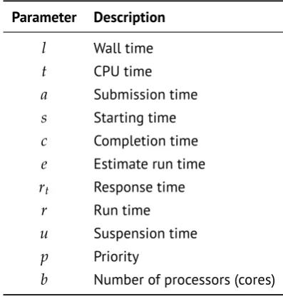
Table 2.1:Scheduling parameters.

Parameter Description

l Wall time

t CPU time

a Submission time s Starting time

c Completion time

e Estimate run time rt Response time

r Run time

u Suspension time

p Priority

b Number of processors (cores)

rectly mentioned by this paper, is that scheduling in practice is very complex, and the building and modifications of an efficient and stable scheduler requires a huge amount of time, money and talent.

2 .

4 Classical scheduling metrics

For the purposes of this thesis, we shall consider the workload as the data about

each jobisubmitted to a supercomputer during a certain time period. Basically, the

workload contains the submission time, ai, the number of requested cores, bi, the

priority,piand the estimated runtime,eiand actual runtime,ri, of each job during the

period. This workload, processed by the scheduler, is called then a supercomputer trace. This trace contains, beyond the information already provided in the workload,

the starting, si, and completion time, ci. Wall time, li, is the elapsed time as

deter-mined by a wall clock. CPU time, ti, is the time consumed by a job and it might

differentiate from wall clock due, for instance, to time-sharing and suspension. If

suspend/resume technique is used, the trace also storesui, which is the total time

a job is suspended. The classical scheduling metrics are average values calculated based on the times found in a trace and they are frequently used to compare the performance of different scheduling algorithms. When comparing algorithms, we also need to introduce the concept of fairness. Considering the jobs in a queue, an algorithm is considered fair if no job with lower priority is allowed to run before a job with higher priority. The algorithm can still be considered fair if the running of the low priority job does not affect the starting time of the job with higher priority, as in the case of Backfill. Table 2.1 summarizes all the main parameters used in this thesis.

(25)

§2.4 Classical scheduling metrics 9

metrics can be easily evaluated. The total time, which is time elapsed from the submission of the first job until the completion of the last job of the trace, takes the form

T =clast_job−af irst_job (2.1)

and it is the most basic metric that can be used to compare two scheduling algorithms.

AlgorithmAwill be considered superior to algorithm B, provide fairness is kept, if

TA < TB. That is the case, for instance, of FCFS with backfill when compared with

the basic FCFS.

The Deadline di is the maximum wall time that a job is allowed to run, and it is

given by

di =si+ui+ei (2.2)

For a trace with njobs, the Average Waiting Time,

wt = n

∑

i=1

si−ai

n (2.3)

basically measures how long a job will stay in the queue. It has been proved [Conway et al., 1967] that, given a workload, the strategy of scheduling the shortest job first (SJF) will result in the lowest values for this metric.

The Response Time,

rt = n

∑

i=1

ci−ai

n (2.4)

takes also into account the runtime of each job and measures the time that takes, on average, for users to obtain their results.

Long jobs have a disproportional influence in the response time. The slowdown,

sd= n

∑

i=1

(ci−ai)/ri

n (2.5)

tries to minimize the influence of these long jobs by dividing the response time of each job by its corresponding runtime.

Weighted Slowdown,

ws= n

∑

i=1

(ci−ai)bi/ri

n (2.6)

is a metric that prioritises jobs requiring a big number of cores by multiplying the slowdown of each job by the number of cores it requires. This is an important metric because the core objective of a HPC facility is solving complex problems that requires a considerable number of cores per job.

(26)

ut = n

∑

i=1

ribi

C T (2.7)

is a metric that evaluates the percentage of the cluster that was effectively used during

the periodT.

2 .

5 Simulation and Emulation

Simulators and emulators try to model, in different levels, the behaviour and the internal workings of a real system.

In a simulator, the functionalities of the real system are highly abstracted. For example, scheduling decisions, unlike on a real system, can occur instantaneously. The internal working of these functionalities in the simulator usually does not reflect how things are implemented on a real system.

An emulator is an intermediate approach between a real system and a simulator. An emulator, like the simulator, can also offer only a few functionalities of the real system, but it tries to reproduce as close as possible the internal workings of the system.

As an example of a real system, we can think about an old valve radio. One can write a software that runs on a computer that simulates the appearance of the radio on the screen. If the power button of the radio simulator is turned clockwise, the radio would turn on and the volume would increase. The real implementation of this feature could bear no resemblance with how things work in a real old radio.

In an emulator, the internal working of some parts of a radio would be mimicked as closely as possible. In this case, we can imagine that the radio emulator wouldn’t turn on the radio immediately because a real old radio would need some time to warm up its valves.

According to [McGregor, 2002], an emulator is a model where some working functions of the model can also be accomplished by the use of components of a real system.

A real HPC system is composed of a supercomputer with one manager node, several processing nodes and a scheduler. Users log on to the manager node and submit their jobs through the scheduler. The scheduler, based on the current state of the running and queued jobs, decides then when and where a job will run.

Simulators built to test scheduling algorithms can be much simpler because most of the details of a real scheduler can be ignored. In the simplest case, the simulator reads a file with a supercomputer trace and applies to its jobs some scheduling algo-rithms. Classical scheduling metrics are then used to compare the performance of the proposed and well-established algorithms. Contrastingly, emulators environments are much more complicated and difficult to build because they try to use, as much as possible, real components.

(27)

§2.6 Scheduling Research Using Simulation 11

This can be classified as emulation since the scheduler operates similarly to the real system.

In this thesis, an emulator was built using 11 virtual machines of an Openstack cloud environment connected together via NFS and running a real scheduler. The emulations were performed by means of a script that reads a trace and runs for each job a special sleep program.

2 .

6 Scheduling Research Using Simulation

Being the easiest way of testing an idea, most of the research in new algorithms is done by means of simulations. The lack of real implementations of algorithms, as discussed below, is a clear evidence of the considerable distance between the development of an idea by means of simulation and its actual implementation in a real scheduler.

This section presents a literature review of the most relevant solutions proposed to improve scheduling research using simulation.

The user runtime estimates have a great impact on how the scheduling occurs. The EASY approach is more efficient when users overestimate, by a great degree, the runtime estimates [Mu’alem and Feitelson, 2001], [Feitelson et al., 2005]. This happens because the overestimation provides a very long reservation time for the first job in the queue. As the running jobs finish well before their expected time, large holes in the scheduling are formed, which can be filled by shorter jobs. This has the net effect of approximating EASY to FCFS [Tsafrir and Feitelson, 2006].

Checkpointing is a technique where a job periodically saves its state in a file. If this job is stopped by any reason before its normal ending, it can later resume its work from the last saved checkpoint. A Checkpoint-based FCFS backfilling algorithm [Niu et al., 2012] presents improvements of up to 40% in the most common metrics. In this algorithm, the backfill is done more aggressively, i.e., filling the holes left by FCFS with jobs that, according to its runtime estimates, would violate the reservation time for the first job in the queue. Due to the user‘s notorious tendency of overestimating the runtime of their jobs, most of these jobs finish before the reservation time comes. The few ones that would be still running after this time would be checkpointed, killed and put back in the queue.

(28)

algorithm. The set of the highest priority running jobs are called sunny load. The set of jobs with priorities lower than any waiting jobs is called shadow load. A backfilled job can change from the shadow to the sunny state during its lifetime. The shadow load is the main cause of unfairness. One approach to solve this problem is to allow the preemption of shadow jobs if this preemption enables higher priorities jobs in the queue to start immediately. A venture backfilling was devised in order to minimize the change of preemption and, consequently, improve system utilisation. This strategy involves the computation of the reservation time of the first job in the queue, a system-generated runtime prediction and careful selection of a job with the biggest probability of successful termination. According to the authors, PV-EASY guaranties fairness, good performance and does not violate reservation times.

Most of the proposed scheduling algorithms focus on improving the so called classical performance metrics, Equations 2.3-2.6. Notably, although being always considered an important feature, fairness has rarely been included as an optimisation criterion for a HPC scheduler. The fair start time (FST) metric [Klusácek and Rudová, 2012] evaluates the influence of arriving jobs on the reservation time for the jobs already in the queue. The unfairness is evaluated as the difference between the FST, which is the reservation time for each job disregarding all later jobs and the actual start time. Another contribution is an optimisation procedure designed to improve the performance of the Conservative Backfilling algorithm. This heuristic uses three parameters, the schedule that will be optimised, the maximum number of iterations and a time limit. In each iteration, one job is randomly removed from its current position and the schedule is immediately compressed while an overall metric, which is a combination of the classical and FST metrics, is calculated. This job is inserted

for a period in ataboolist, which means that it is prevented for a while to be selected

again. The experimental evaluation presented by the authors demonstrated that the proposed extension represented a significant improvement by means of fairness and performance over several existing algorithms, including FCFS, Conservative and EASY backfilling, as well as aggressive backfilling without reservations.

A responsiveness metric, the Schedule Length Ratio (SLR), takes into account the networking delays [Burkimsher et al., 2013]. Through simulations, it was shown that a proposed algorithm that minimizes this metric delivers better responsiveness and fairness than other schedulers that do not rely on user runtime estimates.

Another metric, the thinking time, which is the interval between the response and submission of two consecutive jobs submitted by a single user, can play an important role in the scheduler decisions [Schlagkamp, 2015]. Several simulations showed that this happens because changes in the scheduling will change, in turn, the user’s think time.

(29)

§2.7 Scheduling Research Using Emulation 13

completely ignore the second step leading to results that are not valid in real situa-tions. Therefore, a simulation mode where both steps are present, could help Slurm administrators to find the optimum value for scheduling parameters. This simulation mode could also help Slurm developers in the development of scheduling algorithms. The solution presented in this paper tried to make minimum code changes in Slurm so developers and users would have all Slurm features in the simulation mode. The modifications used the LD PRELOAD functionality of shared objects in UNIX sys-tems. This feature made possible to capture specific function calls exported by shared objects and to replace code when necessary. LD PRELOAD was used to modify the calls to time() function returning a simulated time instead of real time. By using this approach, a trace could run 31 times faster than the original runtime.

[Lucero, 2011] also mentioned that the Moab cluster scheduler supported a sim-ulation mode although it has never worked as described. The reason behind such behaviour was the complexity and high costs associated with keeping the simulation mode in the newer versions. This also has proven to be the case of the simulation mode in Slurm since the development of this feature was abandoned soon after its inception and it is no longer maintained.

2 .

7 Scheduling Research Using Emulation

[Tsafrir and Feitelson, 2006] used a cluster of 32 compute nodes plus one management node to study the influence of two strategies used in schedulers, backfilling and gang scheduling, and the effects of the multiprogramming level. Their results show that the best result was achieved by a combination of both backfilling and gang scheduling with a limited multiprogramming level due to finite memory. One interesting feature of this study was the need of reducing all times from the used workload by a constant factor in order to run the experiments faster. The chosen shrinking factor, 100, was given without any justification and with no analysis of its implications. Contrastingly, this thesis performs a comprehensive study about the implications of shrinking time on the stability of the scheduling metrics, aiming to develop a methodology where this kind of propositions are fully justifiable.

An improved throughput and energy consumption can be achieved through the increasing of memory utilisation, i.e., running more than one job per computing node [Niemi and Hameri, 2012]. This was done at the Worldwide LHC Comput-ing Grid at the Large Hadron Collider at CERN. Due to the fact that this is a HPC facility exclusively dedicated to analyse LHC data, the submitted jobs could be cat-egorised into three groups: CPU-intensive, memory intensive and I/O-intensive. It was proved that running both I/O and CPU intensive jobs in the same node improves both throughput (10-20%) and energy consumption (5-20%). The emulations were performed using a front-end computer, 1 GB network and 2 nodes with 6 CPU cores, 16 gigabytes of memory and 1 TB hard disk each.

(30)

generates multiple bids for a window of jobs at the beginning of the queue. The algorithm maximizes an objective function that uses the jobs priorities. The same authors, in [Soner and Ozturan, 2015], developed a topological aware job scheduling for Slurm. Slurm documentation discourages the configuration of the exact network topology because it leads to slower scheduling. The proposed scheduling method overcomes this limitation and improve the job intercommunication by a judicious job allocation based on the real network topology. In both papers, the authors utilized an emulation mode for Slurm.

More recently, [Rodrigo et al., 2017] presented a scheduling simulation frame-work that encloses all the steps of the scheduling development, providing frame-workload modeling and generation, system simulation, comparative analysis and experiment orchestration. The framework utilizes 17 computing nodes and achieves up to 15 speed-ups over real-time. The authors stated that the limiting factor of the simula-tions speed-up is the scheduling runtime which depends on the number of jobs in the waiting queue. Speed-ups of the same order were also obtained in this thesis without the use of a simulator but our conclusion about the limiting factor differs. Since the number of jobs in the queue was kept constant during our experiments, the limiting factor found was the job submission rate. When this rate exceeds Slurm capacity to process jobs, the cluster nodes will be idle for longer which compromises the evaluation of the classical scheduling metrics. These findings will be discussed in more detail in Section 4.2.4.

2 .

8 Summary

(31)

Chapter3

Design and Implementation

This chapter provides a general overview of the design of the cluster used to emulate a supercomputer as well as the programs and algorithms developed to obtain the results presented in this thesis. Implementations details are given in the software and hardware sections.

3 .

1 Computing Cluster

The design and implementation of the cluster used in this thesis are presented in the next subsections. Subsection 3.1.1 describes the minimum steps to set up a cloud-based cluster. Subsection 3.1.2 shows how to establish a Slurm based cluster at the National Computational Infrastructure (NCI) Nectar Cloud. Finally, using this infrastructure, Subsection 3.1.3 presents a way to emulate a supercomputer size cluster.

3.1.1 Cloud-Based Cluster

A cluster can be set up in a cloud environment in a variety of ways depending on where it is hosted. The most common first step is to create a VM which is going to serve as the cluster head node. This step is followed by the installation and configuration of software packages for parallel computing and communication, like

the OpenMP, MPI andsshbased log in. Computing nodes can then be created using

this head node as a template. Adding the IP addresses of each the computing nodes to the appropriate configuration files in the head node creates a cluster capable of running parallel jobs.

Additionally, a network file system can be mounted in all VMs so the updating, installation and running of packages and programs for resource management can be easily achieved.

3.1.2 NCI Slurm Based Cluster

The National Collaboration Tools and Resources project (Nectar) is an initiative of the Australian Government to provide computational power to Australian researchers

(32)

16 Design and Implementation

HN

CN

slurmcltd

slurmd

CN

slurmd

CN

[image:32.595.73.484.99.358.2]

slurmd

...

Figure 3.1: A normal Slurm based cluster configuration: Oneslurmctlddaemon running in the Head Node (HN) and oneslurmddaemon running in each Computing Node (CN).

through the establishment of a cloud computing infrastructure. Nectar allows re-searches to easily build software and services on the cloud. The Nectar infrastructure is provided through a partnership among research facilities in Australia where NCI is one of its eight nodes.

Nectar uses OpenStack as its cloud software platform. OpenStack is free and open-source software and consists of several components written in Python to control pools of processing, storage, and networking resources. Users can manage it through a web-based dashboard, command-line tools, or web services.

Slurm (Simple Linux Utility for Resource Management), [Jette et al., 2003], is an open-source distributed resource management system software for Linux clusters. Slurm manages the access to computing resources, starts, executes and monitors

jobs, and schedules jobs. The two basic components of Slurm architecture areslurmd,

which is a daemon running on each compute node (CN) and responsible for starting

each job, andslurmctld, a daemon running on a head node (HN).

Munge [Dunlap, 2004] is a software package for the creation, authentication, and validation of credentials in an HPC cluster. Slurm uses Munge to secure the

commu-nication between its main components. Each time a slurmd wants to communicate

with the slurmctld, it first requests a credential from Munge in the local node. This

credential is packed together with the message and send to the head node. Likewise,

a communication received byslurmctldis only processed if the credential contained

in the receiving message is validated by Munge in the head node.

(33)

§3.1 Computing Cluster 17

HN

_slurmcltd

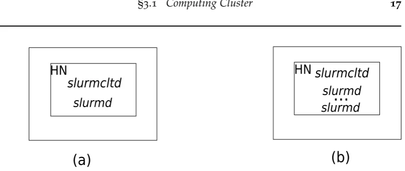
slurmd

...

HN

slurmcltd

slurmd

[image:33.595.124.527.67.237.2]

(a)

(b)

Figure 3.2: Cluster emulation using Slurm Front End and Multiple slurmds features. (a) A singleslurmctldand singleslurmdcan run in the Head Node (HN), or in a desktop, if Slurm is compiled with the Front End option. In this case, the emulated nodes will be set up in the Slurm configuration file but all job management will be accomplished by the singleslurmd. (b) Additionally to the Front End option we can also run multiplesslurmdsin a single computing node with the Multiple Slurmd option. As in (a) the emulated nodes will be also set up in the configuration file, but the management of all the jobs will be shared between the several

slurmds.

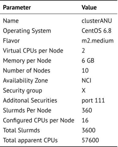
cluster showed in figure 3.1 with one head node and ten processing nodes running CentOS 6.8. All VMs in this cluster have a m2.medium flavour which is how Nectar characterizes a VM. A m2.medium flavour is a VM with 2 CPUs, 6 GB of RAM and 30GB of disk. A volume with 10 GB of space was attached to these nodes. This volume is a storage entity, which is independent of the cluster and can be re-attached to any other VM. The group X is a standard security group in the Nectar cloud and it determines the rules set in the iptables of each VM. The cluster configuration is summarized in Table 3.1.

3.1.3 Cluster Emulation

The emulation of a cluster bigger than its actual size can have many applications. For instance, such bigger clusters can make a better use of its processing power if the jobs running on it are not CPU intensive [Niemi and Hameri, 2012]. The emulation can also help the development of scheduling algorithms. In this case, a sufficiently large cluster could run a supercomputer workload which might provide more realistic results to the developer.

Slurm allows a single node to appear as a cluster by enabling the front end option

(Figure 3.2(a)). This permits the running of one slurmd in the same node as the

slurmctld. Emulated nodes can then be set up in the Slurm configuration file but care must be taken to avoid overloading the slurmd daemon with too many simultaneous jobs. The front end option allows the running of Slurm in a single node or in a desktop computer, but this feature was not used in this thesis because we wanted to

isolate the working of the slurmctldfrom any other sources that could compete for

CPU resources.

Another way of emulating a bigger cluster in Slurm is allowing the running of

(34)

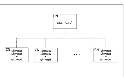
HN

CN

slurmcltd

slurmd CN

...

CN

slurmd slurmd

...

slurmd

slurmd slurmd

...

slurmd

slurmd slurmd

[image:34.595.72.484.99.359.2]

...

Figure 3.3:A cluster emulation with aslurmctldin the head node (HN) and multiplesslurmds

in each computing node (CN).

by the use of the–enable-multiple-slurmdoption. In combination with the Front End

option, we can achieve a configuration like the one showed in Figure 3.2(b), i.e., one

slurmctldand severalslurmdsrunning in a single node.

A greater number of emulated CPUs per node can be achieved by simply

config-uring more CPUs per node in the Slurm configuration file (slurm.conf). Additionally,

the parameterFastScheduleneeds to be set to 2 so Slurm will only consider the

con-figuration of each node that is specified in the concon-figuration file.

Using only the multiple slurmds per node feature, as shown in Figure 3.3, and

setting more CPUs per node than the actual number, we obtained a cluster with 360

slurmdsper node with each one of them configured with 16 CPUs. This combination was sufficient for the emulation of a 3,600 node/57,600 CPU computing cluster. This configuration was very close to NCI‘s supercomputer, Raijin, which, by the time the experiments shown in this thesis were performed, had 3,592 nodes and 57,472 cores. Throughout this thesis, in accordance with Slurm terminology, we will treat CPUs and cores as synonyms.

3 .

2 Hardware platform

(35)

[image:35.595.223.416.135.375.2]

§3.3 Main Programs 19

Table 3.1: Cluster parameters.

Parameter Value

Name clusterANU

Operating System CentOS 6.8

Flavor m2.medium

Virtual CPUs per Node 2

Memory per Node 6 GB

Number of Nodes 10

Availability Zone NCI

Security group X

Additonal Securities port 111

Slurmds Per Node 360

Configured CPUs per Node 16

Total Slurmds 3600

Total apparent CPUs 57600

3 .

3 Main Programs

The main programs and scripts developed during this thesis are presented in the

next subsections. Sigsleepis a program designed to play the role of a job. It responds

to eventual suspensions and writes all context data in a log file. Runtraceis a script

developed to automate the submission of a workload. For each entry in the workload

file, it submits a sigsleep program to the cluster. Calcmets is a program which uses

the data stored in the log file created by sigleep processes to calculate the classical

scheduling metrics.

3.3.1 SigSleep

The emulation of a supercomputer involves the simultaneous running of thousands of programs. A small part of these programs are related to the management of the cluster, e.g. the scheduler, while the vast majority represents incoming jobs. In order to fit all these programs in a finite amount of processors and memory, a dummy program, preferentially one that consumes very little memory and CPU, may be used

to play the role of a job. The most common choice is the sleep program which is

readily available in thebashenvironment. However, this program is not affected by

suspensions as illustrated in Appendix A. As we are using scheduling algorithms that rely on suspensions another solution was required.

This motivated the development of the program sigsleep. Sigsleep (Signal Sleep)

(36)

Algorithm 3.1:A sleep program responsive to suspensions.

1 struct {

2 double suspend,resume;

3 suspend_period∗next;

4 }suspend_period; 5 struct {

6 intid,n_cores,n_suspensions;

7 timespec submission,start,end,runtime;

8 suspend_period∗sus_res;

9 }job_data;

10 suspend_period∗sus_per;

11 Function sighandler(signum)

Input :One nonnegative integersignum Output :The instant the program was suspend

12 sus_per←new(suspend_period); 13 clock_gettime(suspend);

14 sus_per.suspend←suspend; 15 signal(signum,SIG_DFL); 16 kill(getpid(),signum);

17 Programsigsleep(id,priority,n_cores,submission,runtime)

Input :2 integers(id, n_cores), 2 timespec (submission, runtime) and 1 string (priority)

Output :A entry in the log file with the submission, start, end and suspensions times

18 job_data job;

19 clock_gettime(job.start);

20 job ←id,priority,n_cores,submission; 21 job.n_suspensions← −1;

22 job.sus_res←empty_list; 23 remain←runtime; 24 do

25 signal(SIG_TSTP,sighandler); 26 job.n_suspensions++;

27 if job.n_suspension >0then 28 clock_gettime(resume); 29 sus_per.resume←resume;

30 add sus_perto the list job.sus_res;

31 runtime ←remain;

32 whilenanosleep(runtime,remain)==−1; 33 clock_gettime(job.end);

(37)

§3.3 Main Programs 21

sleep, sigsleep keeps track of the suspension periods by detecting and dynamically storing the instants the suspension and resume signals that are sent by Slurm.

The pseudo code for sigsleep is given in Algorithm 3.1 and its source code in

Appendix C. Sigsleep starts with the declaration of structures for storing eventual

suspension periods and the characteristics of the job. The functionsighandler, lines

11 to 16, is registered by sigsleep to handle the signal SIGTSTP (SIGnal Terminal

SToP). This signal must be handled by a program, otherwise, it will be suspended,

which is equivalent to typingCTRL- Zin a terminal. Each timesighandleris called, it

obtains the current suspension time and resets the program to its default behaviour

by using the functionsignal(signum,SIG_DFL).SIG_DFLis a macro that expands into

an integral expression that is not equal to an address of any function. The net result of

callingsignal(signum,SIG_DFL)is to reset the calling program to its default behaviour,

i.e. being able to be suspended. Lastly, sighandler()re-sends the signal SIGTSTP to

finally suspend itself.

Sigsleep, lines 17 to 32, starts by storing its id, priority, number of cores, submission,

start and runtime in ajob_datastruct. It then enters in ado-whileloop controlled by

the functionnanosleep(). Inside this loop, the functionsighanler()is registered and the

value of the number of suspensions incremented. In the first passage, this number

will be zero and, therefore, the instructions inside of theifstatement in line 26 won‘t

be executed. Nanosleep(runtime, remain)suspends the execution of sigsleep until the

time specified byruntimeis elapsed or until a signalSIGTSTPis received. In the last

case, the functionsighandlerwill be called and the program will stop until it receives

a continue (SIGCONT) signal. Once this signal is received, nanosleep() will return-1

and the remaining sleeping time will be given in the parameterremain. This will force

the program to perform a new iteration of the loop, increasing again the number of

suspensions. The condition for theifstatement will be true this time, and the resume

time will be obtained and stored in a simple linked list. This loop will continue until the program is allowed to sleep without any interruptions. The program finishes after

writing in a single log file (LOG_FILE) all data related to the job. The structure of the

log file is a sequence ofjob_data structs interleaved by eventualsuspend_periodstructs.

The fieldn_suspensionsinjob_dataspecifies the number of suspend_periodstructs that

follow that particular struct.

3.3.2 RunWorkload

The submission of an individual job in a Slurm cluster can be accomplished by the

use of thesbatchprogram and a job description file. The main information contained

in this file is the number of cores, nodes, priority and the program to be run.

Abashscript, calledrunworkload, was developed to automate the task of submitting

all jobs contained in a workload. Additional parameters were also introduced to enable studies on runtime shrinkage. Beyond the workload filename, the user can also provide the initial and final shrinking factors and a step. For instance, typing

(38)

Algorithm 3.2:A script for workload emulation.

1 Function sleep_submission_period(j, trace_ini)

Input :Two nonnegative integers, submission period and the start of the trace

Output :sleeping for regular intervals

2 sdj←trace_ini+warmup_period+ (dri f t+submission_period)∗j; 3 sleep(sdj−now);

4 ProgramrunWorkload(w_file,ini, end, step)

Input :1 string (workload filename), 3 integers (initial, end and step shrink factors)

Output :A file containing the trace emulation

5 fori←initoendbystep do 6 n_group,n_jobs←0; 7 trace_ini←now;

8 foreach job in w_filedo

9 n_jobs++;

10 shrink job‘s submission time, expected runtime and runtime byi;

11 if(n_jobs >= n_warm_up)and(n_jobs % sub_group ==0)then 12 sleep_submission_period(n_group,trace_ini);

13 n_group++;

14 write submission script, job_description, with job info;

(39)

§3.4 Software platform 23

actual running times as described in the filework_file. These times will be decreased

by steps of 10% until the final shrinkage factor of 50% in the subsequent output files.

Runworkload, presented in Algorithm 3.2, starts by submitting a preconfigured

number of jobs as warm up jobs (n_warm_up). Once the warm up period (warmup_period)

finishes, the following jobs are then submitted in groups (sub_group) in regular

inter-vals (sub_period). The objective of the functionsleep_submission_period()is to guarantee

that the start of a new submission period is done in terms of wall time instead of a period relative to the last submission. This is necessary since the submission time for each job, line 15, is arbitrary and depends on how busy Slurm is. The importance

of setting the sleeping periods in this way and the necessity of the drift parameter

will be evidenced during the discussion of the emulation methodology presented in Section 4.2.4.

3.3.3 CalcMets

Calcmets, Algorithm 3.3, is a program that evaluates the classical scheduling metrics, i.e. average waiting time, response time, slowdown, weigthed slowdown and cluster utilization. The metrics are calculated from the trace data generated by the running

of several sigsleep programs. This trace is a binary file composed by a sequence of

job_datastructs (1-4) interleaved by sequences ofsuspend_periodstructs (5-9).

The logic of this program is straightforward. The information about the jobs

are stored in an array of job_data structs (16). All data concerning suspensions of

a particular job is stored in a linked list accessed by the field sus_res. Once this

information is read from the trace file, the scheduling metrics are evaluated according to the formulas presented in section 2.4.

3 .

4 Software platform

All programs were compiled using the GNU Compiler Collection (GCC). Programs

using theclock_gettimefunction were compiled with the flags-lrt.

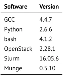
The versions of all software used in this thesis are summarized in table 3.2.

3 .

5 Summary

(40)

Algorithm 3.3:An algorithm for classical scheduling metrics evaluation

1 struct {

2 double suspend,resume;

3 suspend_period∗next;

4 }suspend_period; 5 struct {

6 intid,n_cores,n_suspensions;

7 timespec submission,start,end,runtime;

8 suspend_period∗sus_res;

9 }job_data;

10 Function read_jobs(trace, jobs)

Input :trace filename

Output :array of job_data

11 whilenot end of tracedo

12 read job data and store in jobs[i++];

13 for j←1tojobs[i].n_suspensionsdo

14 read and add to job[i].sus_resa new suspend_period node;

15 Programcalcmets(trace)

Input :Trace File Name

Output :Classical Scheduling Metrics

16 job_data jobs[];

17 read_jobs(trace,jobs);

[image:40.595.224.330.584.711.2]

18 evaluate classical metrics;

Table 3.2:Software Platforms

Software Version

GCC 4.4.7

Python 2.6.6

bash 4.1.2

OpenStack 2.28.1

Slurm 16.05.6

(41)

Chapter4

Experimental Methodology

This chapter characterizes the experimental workload and details the methodology used in the emulations presented in this thesis.

4 .

1 Experimental Workload Characterization

We used a workload containing 4,417,018 jobs submitted to NCI‘s supercomputer between April 1, 2016, and November 1, 2016. This workload contains, among other information, the submission time, number of requested cores, and estimated and actual runtimes for each job. Figure 4.1 shows the distribution of the number of jobs per CPU count in a logarithmic scale.

One particular feature of this workload is the great presence of one-core jobs, which make up almost 50% of all jobs submitted during the period. This is a charac-teristic of NCI which not only provides HPC services, but also provides 8 petabytes of high-performance storage services. Most of the access to the data is made by one-core jobs. Table 4.1 displays the most common job sizes and their respective percentage of the total number of jobs. It is worth noting that, out of 193 different job sizes presented in the workload, the number of jobs requesting 1, 2, 4, 8, 16, 48 and 64 cores accounts for 90% of all jobs submitted.

[image:41.595.242.393.619.738.2]

This job size distribution could lead to the wrong conclusion that most of the work done at NCI do not actually need a supercomputer. Nevertheless, Table 4.2 shows

Table 4.1:Job size and its percentage of total jobs

Job Size (cores) % of Total Jobs (%)

1 49

2 11

4 5

8 7

16 8

48 4

64 6

all rest 10

(42)

[image:42.595.89.468.131.318.2]

26 Experimental Methodology

Figure 4.1:Raijin’s job size distribution (Y axis is logarithmic)

the job distribution in terms of service units (S.U.), which is the runtime of a job multiplied by the number of cores used. This data demonstrates that most of the work done at NCI‘s supercomputer is performed by jobs that use a considerable number of cores. One core jobs, on the other hand, use only 1.6% of NCI‘s computational power.

One interesting feature of this workload is the distribution of the job‘s submission time along the day. It would be reasonable to expect a peak during working hours, yet Figure 4.2 shows a fairly uniform distribution.

[image:42.595.80.477.486.708.2]

(43)

[image:43.595.178.457.136.351.2]

§4.2 Classical Metrics Artefacts 27

Table 4.2: Job size and its percentage of total Service Units (S.U.)

Job Size (cores) Runtime (106s) S.U. (109cores*s) % of Total S.U.

64 2416.1 154.6 16.0

128 850.1 108.8 11.2

320 188.4 60.3 6.3

256 235.0 60.2 6.2

16 3154.5 50.5 5.2

512 82.9 42.6 4.4

8 5243.2 41.9 4.3

32 915.7 29.3 3.0

48 485.7 23.3 2.4

384 60.5 23.2 2.4

1008 17.7 17.8 1.9

1024 17.1 17.5 1.8

192 82.0 15.8 1.6

1 15355.0 15.3 1.6

3200 4.5 14.6 1.5

all rest 30.2

As already explained in Section 2.3, a scheduler using the Backfill algorithm demands an estimate for the runtime of a job at its submission time. Figure 4.3 exemplifies the users‘ notorious behaviour of largely overestimating the runtime values. This graph shows the percentage of the total jobs for each interval of the ratio between the actual runtime (RT) and the runtime estimate (ER). For instance, almost 60% of all jobs submitted have their runtime estimates more or equal than 10 times the actual runtimes, which is the first interval (0.0,0.1] showed in Figure 4.3. On the other end, only 0.7% have this ratio falling within the (0.9,1.0] interval which could be considered a very good estimate. This behaviour is easily explained by the fact that overestimating the running time incurs no penalty, whilst users might have their jobs killed if their actual runtime exceeds its runtime estimate. Usually, a job will not be killed as soon as this situation occurs but after a grace period, which explains the (1.0,1.1] interval.

4 .

2 Classical Metrics Artefacts

(44)

28 Experimental Methodology

Figure 4.3: Users’ accuracy for their job runtime estimates. X-axis contains the intervals for the ratio between the actual runtime and estimated runtime. Y-axis shows the percentage of these jobs in relation to the total number of jobs in the workload. For instance, all jobs with a runtime estimate equal or bigger than 10 times the actual runtime are grouped in the (0.0,0.1] interval which represents 58% of all submitted jobs.

[image:44.595.78.476.99.350.2]

4.2.1 Concurrency

Table 4.3:Stability of the classical metrics over the course of 5 consecutive runs. The columns are Waiting Time (WT), Response Time (RT), Slowdown (SD), Weighted Slowdown (WS) and Utilization (UT). The last 4 rows are the Average (AVE), Standard Deviation (SSD), Relative Standard Deviation (RSD) and the Confidence Interval with a level of Confidence of 95% (C95) . This notation will be repeated in the following tables.

Run WT (s) RT (s) SD WS UT (%)

1 1261.1 1389.3 64.8 103.5 90.2 2 1286.8 1415.0 67.4 115.3 92.2 3 1256.0 1384.1 67.7 106.8 91.3 4 1294.7 1422.8 67.7 112.2 90.7 5 1304.5 1432.6 64.9 109.9 91.5

AVE 1280.6 1408.8 66.5 109.5 91.2

SSD 48.9 18.9 1.4 4.1 0.7

RSD (%) 1.5 1.3 2.0 3.8 0.8

C95 60.7 23.5 1.7 5.1 0.9

(45)

§4.2 Classical Metrics Artefacts 29

metrics varied from one experiment to the next even when all parameters were kept the same due to the non-deterministic nature of time-dependent experiments in distributed systems. This shows that emulation presents relevant additional features when compared with simulation, which usually displays a deterministic behaviour.

Tables 4.3, 4.4, 4.5, and 4.6 utilize a 1,000 job workload running in a 3,000 node/3,000 CPU cluster. Table 4.3 presents the results for five consecutive experi-ments with all the cluster configuration parameters kept constant. All the metrics display a low Relative Standard Deviation (RSD). The low values for the RSD and the similar values between the standard deviation (SSD) and the confidential interval with a level of confidence of 95% (C95) indicates that these metrics are sufficiently stable in relation to concurrency to be used in comparisons to different scheduling algorithms. A particular result shown in this table is the high stability of the cluster utilization metric, which displays a RSD of only 0.8%. As we will show later, the utilization also displays a very stable behaviour in relation to all the other artefacts studied.

4.2.2 Submission order

As discussed in [Frachtenberg and Feitelson, 2005], workloads from different HPC facilities can be quite different from each other. These differences can influence the performance of the scheduling algorithms as it was found in [Mu’alem and Feitelson, 2001], where the relative performance of EASY and Conservative Backfill depended on the workload used and on the performance metrics.

This motivated us to investigate the behaviour of the classical metrics in relation to the submission order of the jobs for a particular workload. From a single workload, we generate 10 different workloads by randomly changing the submission order of the jobs. We kept the submission times equally distributed along the trace duration. This was done for two reasons: First, Figure 4.2 shows a very uniform submission time distribution over a 24 hours period while the other reason is related with the dif-ferences between a simulation and the actual working of a real RMS. In a simulation, the scheduler can run the scheduling algorithm as soon as a new job arrives. However, there are many more tasks, beyond scheduling, that a real RMS must perform. This imposes an empirical limit to the number of jobs in the queue that can be sched-uled as soon as a running job completes. For instance, Slurm performs two types of scheduling, one fast that only takes into account a small percentage of the whole queue and one more comprehensive that involves the whole queue, but that is done only at preconfigured intervals. The Slurm documentation recommends disabling the fast scheduling for high throughput clusters, which can be easily accomplished

by setting a parameter, defer, in the configuration file. We use this high throughput

Supercomputer Emulation For Evaluating Scheduling Algorithms