This is a repository copy of Frequency domain analysis of a dimensionless cubic nonlinear
damping system subject to harmonic input.
White Rose Research Online URL for this paper: http://eprints.whiterose.ac.uk/74691/
Monograph:
Jing, X.J. and Lang, Z.Q. (2008) Frequency domain analysis of a dimensionless cubic nonlinear damping system subject to harmonic input. Research Report. ACSE Research Report no. 971 . Automatic Control and Systems Engineering, University of Sheffield
Reuse
Unless indicated otherwise, fulltext items are protected by copyright with all rights reserved. The copyright exception in section 29 of the Copyright, Designs and Patents Act 1988 allows the making of a single copy solely for the purpose of non-commercial research or private study within the limits of fair dealing. The publisher or other rights-holder may allow further reproduction and re-use of this version - refer to the White Rose Research Online record for this item. Where records identify the publisher as the copyright holder, users can verify any specific terms of use on the publisher’s website.
Takedown
If you consider content in White Rose Research Online to be in breach of UK law, please notify us by
Frequency Domain Analysis of a
Dimensionless Cubic Nonlinear Damping
System Subject to Harmonic Input
X. J. Jing and Z. Q. Lang
Department of Automatic Control and Systems Engineering The University of Sheffield
Mappin Street, Sheffield S1 3JD, UK
Frequency Domain Analysis of a
Dimensionless Cubic Nonlinear Damping
System Subject to Harmonic Input
Xing Jian Jing* and Zi Qiang Lang
Department of Automatic Control and Systems Engineering, University of Sheffield Mappin Street, Sheffield, S1 3JD, U.K.
Abstract: The effects of cubic nonlinear damping on the system output spectrum are
theoretically studied through a dimensionless mass-spring-damping system model subject to a harmonic input, based on the Volterra series approximation. It is for the first time shown theoretically that the cubic nonlinear damping has little effect on the system output spectrum at high or low frequencies but drives the system output spectrum to be an alternative series at the natural frequency 1 such that the system output spectrum can be suppressed by the cubic damping.
Keywords: Cubic nonlinear damping, Output frequency response, Alternative series
1 Introduction
2 A dimensionless vibration system and its frequency response
functions
Consider a SDOF nonlinear mass-spring-damping system as show in Figure 1. The dynamics of the system can be described by
) ( ) ( ) ( ) ) ( ( )
(t c1 c2zt 2 zt k zt ut
z
m&& ′ + + & ′ & ′ + c ′ = ′
In this study, suppose the input u(t) to be a harmonic excitation given by
) sin( )
(t A t
u ′ = Ω′
which can be transformed into a dimensionless format as
) ( ) ( ) ( ) ( )
(t 1x t 2x t 3 xt u t
x& + & + & + =
& ξ ξ (1a)
) sin( 1 )
( t
k t u
c
ω
= (1b) where
A z x= ,
m kc
=
Ω0 , t=Ω0t′, 0
Ω Ω =
ω ,
m k
c
c
1 1 =
ξ , 2 2
2 d
c
F m k c
=
ξ . For convenience, let
kc=1 in what follows. Consider the output of interest for model (1ab) as
) ( ) ( ) ( )
(t 1x t 2x3 t xt
y =ξ & +ξ & + (1c)
which is the transmitted force from u(t) to the base. The dimensionless model (1a) can be found in many engineering systems, usually acting or known as a vibration isolator [3, 12] as shown in Figure 1 with a nonlinear damping, or be found in circuit systems as shown in Figure 2 with a nonlinear resistor.
Fig. 1 A mass-spring-damping system with nonlinear damping
Figure 2. A similar circuit system with nonlinear resistor
Note that there is a cubic nonlinear damping terms in (1a). The objective of this study is to analyze the effect of the nonlinear damping on the system output response in the frequency domain, and therefore to demonstrate some notable advantages of the nonlinear damping compared with the linear damping known in the literature.
f(.)
kc z(t)
u(t)
m
C L
R u(t)
The frequency domain analysis of nonlinear systems can be carried out based on the Volterra series expansion theory. It is known that, nonlinear systems can be approximated by a Volterra series up to maximum order N in the neighbourhood of the zero equilibrium [2] as
∑
=∫
∫
−∞∞∏
=∞ ∞
− −
= N
n
n
i
i i n
n ut d
h t
y
1 1
1, , ) ( )
( )
( L τ Lτ τ τ (2) where hn(τ1,L,τn) is called the nth-order Volterra kernel. The generalized frequency
response function (GFRF) is defined as [13]
∫
∫
−∞∞∞ ∞
− − + +
= n n n n n
n
n j j h j d d
H ( ω1,L, ω ) L (τ1,L,τ )exp( (ω1τ1 L ωτ )) τ1L τ (3)
which provides a basis for the frequency domain analysis of nonlinear systems. In order to conduct the frequency domain analysis of the cubic nonlinear damping, the GFRFs and output spectrum of system (1) can be obtained by using some recently developed results[15-17]. These are summarized in the following Lemmas.
Lemma 1. The GFRFs for the relationship between u(t) and y(t) of model (1) can be
determined as: for n=0,1,2,3,…
0 ) , ,
( 1 2
2 n =
y
n j j
H ω L ω (4) and
(
1 ( ))
( , , ) ( ( )) ( , , )) , , (
1 2 1 3 , 1 2 2 1
2 1 1 2 1 2 1
1
1 2 1 1 2
+ +
+ +
+ +
+
+ ⋅
+ + ⋅ +
= n n n
x n n
n y
n
j j H n j
j H j
j j j H
ω ω ξ
δ δ ω ω ω
ω ξ
ω ω
L L
L L
(5a)
(5a) can also be written as for n>0,
∑ ∏
− + == =
+ +
+ +
+ +
+ + +
∑
+ + +
+ + + −
= 2 1
1 2
1 3
1
1 1
1 2 1
1 2
2 1 2 1
2
1 2 1 1 2
1
) )(
, , ( )
(
) (
) , , (
n
n r r
r i
r X X
r X X
x r n
n
n n y
n
i p
i i
i j j j j
H j
j L
j j
j j H
L
L L
L L L
ω ω
ω ω
ω ω
ω ω
ξ
ω ω
(5b)
where for n=0, 1,2,3,…
0 ) , ,
( 1 2
2 n =
x
n j j
H ω L ω (6a)
) (
) , , ( )
, , (
1 2 1
1 2
1 2 1 3 , 1 2 2 1 2 1 1 2
+ +
+ +
+
+ = + +
n n
n n
n x
n
j j
L
j j H j
j H
ω ω
ω ω ξ
ω ω
L L
L (6b)
∑
− =+ +
− +
+ ⋅ = + +
1 2
1
1 1 2 1 2 , 1 2 1
3 , 1
2 () ( , , ) ( , , )( )
n
i
i n
i i n i x
i
n H j j H j j j j
H ω L ω ω L ω ω L ω (6c)
1
) )(
, , ( )
, ,
( 1 2 1 2 1 1 2 1 1 2 1
1 , 1 2
k n n
x n n
n j j H j j j j
H + ω L ω + = + ω L ω + ω +L+ ω + (6d)
) (
1 ) (
1 1 1
1 ω ω
j L j
Hx = − (6e)
L2n+1( jω1+L+ jω2n+1)=
(
)
2 1 2 11 2 1
1( ) ( )
1+ + + + + + + +
− ξ jω L jω n jω L jω n (6f) Proof. See Appendix A.
Therefore, based on (4-6), the GFRFs for the relationship between y(t) and u(t), can be determined up to any high orders. According to the results in [15, 17], and noting that there is only one nonlinear term with coefficient ξ2, it can be obtained that the nth-order GFRF for the relationship between y(t) and u(t) can be expressed as for n=0,1,2,3,…
) , , ( )
, ,
( 1 2 1 2 2 1 1 2 1
1
2 + + = ⋅ n+ n+
n n y
n j j f j j
0 ) , ,
( 1 2
2 n =
y
n j j
H ω L ω (7b) From the results in [16], it can be seen that f2n+1(jω1,L,jω2n+1) is a function of
) (
1 i x
j
H ω with degree 2n+1 and also a function of Lj(.) with degree n. Also from the recursive computation above, it can be verified that the complex valued function f2n+1(jω1,L,jω2n+1)in (7a) can be written as
∑
∏
∏
∏
− ≤ ≤ + ∈
−
= + +
−
= +
= + +
+
− + + ⋅ + +
+ + ⋅
⋅ +
+ −
=
} 1 1 1 2 {
) , , (
1
1
) ( )
1 ( 1
2 1
1 2
1
1
) ( )
1 ( 1
2
1
1 1 2
1 2 1
1 2 1 1 2
1
1 ( ) ( )
) (
) ( ) ( ) (
) , , (
n k k j
j j
n
i
j l l
j n
n
n
i
j l l
n
i
i x n
n n
i n
i i
i
j j
L j
j L
j j
j H j j
j j j f
L L L
L L
L
ω ω
ω ω
ω ω
ω ω
ω ω
ω ω
(8)
Assume that f1(jω1) H1(jω1)
x
= for n=0 in (7a). This can also be proved rigorously by mathematical induction which is straightforward. Equation (8) can be determined explicitly from equations (4-6).
Lemma 2. The system output frequency response is
⎣ ⎦
∑
−=
+
= 2
1
1
0( ) ( )
) (
N
n n j
Y j
Y j
Y ω ω ω (9a)
2
) ( ) 1 ( )
( 1 1
0
ω ω ξ
ω jF j H j
j Y
x d +
−
= (9b)
(
)
∑
∑ ∏
= + +
− ≤ ≤ + ∈
−
= +
+
+ − + +
+ + ⋅
⋅ ⋅
⋅ ⋅
=
ω ω
ω ω ω
ω ω
ω
ω ω ω ω ω ξ
ω
1 2
1 1 1
} 1 1 1 2 {
) , , (
1
1 (1) ( )
) ( )
1 ( 1
2 1
2 1 1
2 1 2 2
) (
) (
) ( ) ( )
( ) (
2 ) ( )
(
n k k
i
n i i
i
n k k j
j j
n
i j l l j
j l l
x n x n
n d n n
j j
L
j j
j L
j j H j j H j F
j j
Y
L L L
L (9c)
for n>0 with assumption that
∑ ∏
− ≤ ≤ + ∈
−
=
− + +
+ +
} 1 1 1 2 {
) , , (
1
1 (1) ( )
) ( )
1 (
1
1 ( )
n k k j
j j
n
i j l l j
j l l
i
n i i
i
j j
L
j j
L L
L
ω ω
ω ω
=1 when n=1.
Proof. See Appendix B.
Equations (9a-c) are a qualitative description of the output spectrum of model (1), which facilitates the analysis in the following section. Y0(jω) denotes the effect of the linear part of the system, and Yn(jω)for n=1,2,3,… denotes the effect of the nonlinear damping. The
detailed output spectrum can be determined by following the proof of Lemma 2 in Appendix B.
3 Analysis based on the frequency response functions
From Equations (9a-c), it can be seen that the nonlinear damping drives the system output spectrum to be an infinite series. When the nonlinear damping is zero, i.e., ξ2 =0, then the system is recovered to a linear system whose output spectrum is Y0(jω). In order to
(1) Magnitude ofY(jω) when |ω-1| is much larger than 0
It follows from (6f) that
2 1 2 2 2 1 1 2 1 1
2+ (jω + + jω +)ω1+ +ω2+1=Ω=1+ξ (jΩ)+(jΩ) = (1−Ω ) +(ξΩ)
L
n
n
n L L
then ⎪⎩ ⎪ ⎨ ⎧ << Ω ≥ Ω + >> Ω Ω ≥ Ω + Ω ≈ Ω + 1 for 1 ) ( 1 1 for ) ( ) ( ) ( 2 1 2 2 1 2 2 1 2 ξ ξ j
Ln (10a)
and it follows from (6e) that
⎪ ⎩ ⎪ ⎨ ⎧ << >> ≤ = 1 for 1 1 for 1 ) ( 1 ) ( 1 1 2 1 1 1 1 1 ω ω ω ω ω j L j
Hx (10b)
Consider two cases in the following: ω>>1and ω<<1. For comparison, study the magnitude of the linear part in the output spectrum at first. It follows from (9b) that
2 1 2 2 2 1 2 1 2 1 1 1 0 ) ( ) 1 ( 2 ) ( 1 ) ( ) ( 1 2 ) ( 1 2 ) ( ) 1 ( ) ( ω ξ ω ω ξ ω ω ξ ω ξ ω ω ξ ω + − + = + + + = + − = j j j H j jF j Y x
d (11)
When ξ2=0, the magnitude of the system output spectrum will be guided by (11). It can be seen that, an increase of the linear damping parameterξ1will result in a decrease of the magnitude at ω=1 but an increase of the magnitude at higher frequency, and
5 . 0 ) (
0 jω →
Y when ω→0 . However, the nonlinear damping will not bring noticeable increase for the magnitude of the system output spectrum at higher or lower frequency than 1 as discussed below.
Case 1: high frequency response, i.e.,ω>>1
Using (10) and (9c), it can be derived that for n>0 andω>>1
∑
∑ ∏
∑
∑ ∏
= + + − ≤ ≤ + ∈ − = + − + + = + + − ≤ ≤ + ∈ − = + + + + − + − + + + + ⋅ ⋅ ⋅ ⋅ ≈ + + + + ⋅ ⋅ ⋅ ⋅ ≤ ω ω ω ω ω ω ω ω ω ω ω ω ω ω ξ ω ω ω ω ω ω ω ω ξ ω 1 21 1 1
1 2
1 1 1
} 1 1 1 2 { ) , , ( 1 1 2 ) ( ) 1 ( ) ( ) 1 ( 2 2 1 2 2 1 2 1 2 2 } 1 1 1 2 { ) , , ( 1
1 (1) ( )
) ( ) 1 ( 1 2 1 2 1 1 2 1 2 2 ) ( ) ( ) ( 2 ) ( ) ( ) ( ) ( ) ( 2 ) ( ) ( n k k i n i i n k k i
n i i
i n k k j j j n
i l l j
j l l n n n d n n k k j j j n
i j l l j
j l l n x n n d n n F j j L j L j H F j Y L L L L L L L L ) 12 ( 1 1 2 1 1 1 2 1 } 1 1 1 2 { ) , , ( 1 1 2 1 2 2 } 1 1 1 2 { ) , , ( 1
1 (1) ( ) 1 2 1 2 2 1 1 1 2 1 1 1 1 2 1 a n k k j j j n n n n n k k j j j n
i l l j
n n n i n n k k i n i n k k
∑
∑
∑ ∏
∑
− ≤ ≤ + ∈ − = + + + + − ≤ ≤ + ∈ − = = + + + + − + − + ⋅ ⋅ ⋅ < + + ⋅ ⋅ ⋅ ≈ L L L L L ω ω ξ ω ω ω ξ ω ω ω ω ω ω From (12a), it can be seen that, when ω>>1 and for a boundedξ2, Yn(jω) →0, thus
) ( )
(jω Y0 jω
Y → . Therefore, it can be concluded that, after the nonlinear damping is
introduced. Thus the nonlinear damping has little effect on the output spectrum of system (1) at high frequency. This may be held even for a larger but finiteξ2.
Case 2: low frequency response, i.e.,ω<<1
Similarly, using (10) and (9c), it can be derived that for n>0 andω<<1
) 12 ( 2
1
1 ) (
2 ) (
) (
) (
) ( ) (
2 ) ( ) (
} 1 1 1 2 {
) , , (
1
1
) ( )
1 ( 3
2 1 2 2
} 1 1 1 2 {
) , , (
1
1
) ( )
1 ( 2
1 2
1 2
1 2 2
} 1 1 1 2 {
) , , (
1
1 (1) ( )
) ( )
1 (
1
2 1 2 1 1 2
1 2 2
1 1 1 2 1
1 2
1 1 1
1 2
1 1 1
b F
j j
L j
L j H F
j Y
n k k j
j j
n
i
j l l
n n n
n k k j
j j
n
i
j l l
n n
n d n
n k k j
j j
n
i j l l j
j l l
n x n
n d n n
i n
i n
k k
n k k
i n
i n
k k
i
n i i
i
∑ ∏
∑
∑
∑ ∏
∑
∑ ∏
− ≤ ≤ + ∈
−
= =
+ + + +
= + +
− ≤ ≤ + ∈
−
= +
+ +
= + +
− ≤ ≤ + ∈
−
= +
+ +
− +
+ −
+ −
+ + ⋅
⋅ ⋅ =
+ + ⋅
⋅ ⋅ ⋅
≤
+ +
+ + ⋅
⋅ ⋅
⋅ ≤
L L
L L
L L
L
L
L L
ω ω
ω ξ
ω ω
ω ω ξ
ω ω
ω ω
ω ω ω
ω ξ
ω
ω ω ω
ω ω ω
ω ω ω
From (12b), it can be seen that, when ω<<1 and for a boundedξ2, Yn(jω) →0, thus
) ( )
(jω Y0 jω
Y → . Therefore, after the nonlinear damping is introduced, the magnitude of system output spectrum is not obviously increased at lower frequencies compared with the case without the nonlinear damping being introduced. Thus the nonlinear damping has also little effect on the output spectrum of system (1) at lower frequency.
The following discussion will show that a proper nonlinear damping will reduce the magnitude of system output spectrum at frequencyω≈1.
(2) The frequency characteristic of Y(jω) at frequency ω≈1
For any υ∈C (the set of all the complex numbers), define ⎥ ⎦ ⎤ ⎢
⎣ ⎡ =
)) ( ( 0
0 ))
( ( )
(
υ υ
υ
IMAG sign REAL
sign
signc (13)
where
⎩ ⎨ ⎧
< −
≥ +
=
0 1
0 1
) (
x x x
sign for x∈ℜ, REAL(υ)is the real part of υ and IMAG(υ)is the
imaginary part of υ. Obviously, signc(.)≠0, signc(.)-1 exists and signc(.)-1=signc(.). Definition 1. Considering a series S in C , i.e., S=s0+s1+s2+s3+……, if the following
conditions hold,
(1)REAL(sn)IMAG(sn)REAL(sn+1)IMAG(sn+1)≠0, and additionally signc(sn)signc(sn+1)=-1 (2) 0
) ( ) ( ) ( )
(sn IMAGsn REAL sn+1 IMAGsn+1 =
REAL , and additionally
sign(REAL(sn)REAL(sn+1))=−1or sign(IMAG(sn)IMAG(sn+1))=−1
then it is said to be an alternating series, where 1 is two-dimensional unitary matrix.
The traditional definition for the alternating series can refer to [18]. The following result can be established.
Theorem 1. Consider the dimensionless system (1). At around natural frequency 1, the cubic nonlinear damping drives the system output spectrum to be an alternating series if the linear damping parameter ξ1 is sufficiently small, i.e., ξ1<<3.
Proof. By using this function, it can be derived that
(
)
∑
∑ ∏
= + + = + ∈ − = + + + − ⎥ ⎥ ⎦ ⎤ + + + + ⋅ ⋅ ⋅ ⋅ ⎢ ⎣ ⎡ ⋅ = ω ωω ω ω
ω ω ω ω ω ω ω ω ξ ω 1 2
1 1 1
} ,... 2 , 1 1 2 { ) , , ( 1
1 (1) ( )
) ( ) 1 ( 1 2 1 2 1 1 2 1 2 2 ) ( ) ( ) ( ) ( ) ( ) ( 2 ) ( )) ( ( n k k i
n i i
i n n j j j n
i j l l j
j l l x n x n n d n n j j L j j j L j j H j j H j F j signc j Y signc
L L L
L
which further yields
⎟⎟ ⎟ ⎟ ⎠ ⎞ ⎜⎜ ⎜ ⎜ ⎝ ⎛ + + + + ⋅ ⎟⎟ ⎟ ⎟ ⎠ ⎞ ⎜⎜ ⎜ ⎜ ⎝ ⎛ + + + + = =
∑
∑ ∏
∑
∑ ∏
= + + = + ∈ − = = + + = + ∈ = + − + + − + ω ω ω ω ω ω ω ω ω ω ω ω ω ω ω ω ω ω 1 21 1 1
3 2 1 1 } ,... 2 , 1 1 2 { ) , , ( 1
1 (1) ( )
) ( ) 1 ( } ,... 2 , 0 3 2 { ) , ,
( 1 (1) ( )
) ( ) 1 ( 1 1 1 ) ( ) ( )) ( ( )) ( ( )) ( ( )) ( ( n k k i
n i i
i n
k k
i
n i i
i n n j j j n
i j l l j
j l l n n j j j n
i j l l j
j l l n n n n j j L j j signc j j L j j signc j Y signc j Y signc j Y signc j Y signc L L L L L L L L (14)
Note that ω ∈{ω,−ω}
i
k , and the condition ωk1 +L+ωk2n+1 =ω, thus there are n+1 frequencies equal to ω and n frequencies equal to -ω . jωl(1)+L+ jωl(ji) is the summation of ji frequencies chosen from the 2n+1 frequencies, where ji is an odd number. Note also that
∑
= + + ω + ω ω1 2 1
(.)
n k k L
includes all the possible cases for different values ofω ∈{ω,−ω}
i
k such
thatωk1 +L+ωk2n+1 =ω. It can be verified that jωl(1)+L+jωl(ji) = pjω for some odd integer p satisfying |p|<n+2. Thus
⎟⎟ ⎟ ⎟ ⎠ ⎞ ⎜⎜ ⎜ ⎜ ⎝ ⎛ − − = ⎟⎟ ⎟ ⎟ ⎠ ⎞ ⎜⎜ ⎜ ⎜ ⎝ ⎛ + − − = ⎟⎟ ⎟ ⎟ ⎠ ⎞ ⎜⎜ ⎜ ⎜ ⎝ ⎛ + + + +
∑
∑ ∏
∑
∑ ∏
∑
∑ ∏
= + + = + ∈ − = − = + + = + ∈ − = − = + + = + ∈ − = + − + − + − ω ω ω ω ω ω ω ω ω ω ω ω ξ ω ω ω ω ω ω 1 21 1 1
1 2
1 1 1
1 2
1 1 1
} ,... 2 , 1 1 2 { ) , , ( 1 1 1 1 } ,... 2 , 1 1 2 { ) , , ( 1 1 1 2 1 } ,... 2 , 1 1 2 { ) , , ( 1
1 (1) ( )
) ( ) 1 ( ) ( ) 1 ( ) ( ) ( 1 ) 1 ( ) ( n k k i n i i n k k i
n i i
i n
k k
i
n i i
i n n j j j n i ij ij n n n j j j n
i ij ij
ij n n n j j j n
i j l l j
j l l jp L jp signc jp p jp signc j j L j j signc L L L L
L L L
L (15) Consider ) ( 1 ω ω ij ij jp L jp
− at ω≈1where pij is an odd integer satisfying |pij|<n+2.
ij ij j ij ij p sign j ij ij ij ij ij ij e p p e p p j p jp jp L jp θ ξ ξ ω ω π 2 1 2 2 ) ( 1 2
1( ) 1 (1 ) ( )
where
⎪⎩ ⎪ ⎨ ⎧
≥ −
= =
3 if ) )( (
1 if 2
) (
ij ij
ij
ij ij
ij
p p
sign
p p
sign
δ π π
θ ,δij ≥0andδij →0when pij >>1andξ1 <<1. Thus 1
1
1 )
( ω ξ
ω
= − ij
ij
jp L
jp
when pij =1 (16a)
and
ij p sign j
ij p sign j
ij ij
p e p
e jp L
jp ij ij ( ij) ( ij) 2
1 2
) ( ) (
1
2 2
) (
δ
δ π
π
ξ ω
ω − − − −
≤ + ≈
− when pij >1 (16b)
1
± =
ij
p corresponds to jωl(1)+L+ jωl(j) =±jω, and
) (
1 ω
ω
j L
j
± −
±
is a positive real number in
this case. However, pij ≥3 corresponds to jωl(1) +L+ jωl(j) = jpijω , and
) (
1 ω
ω
ij ij
jp L
jp
− is
approximately a pure negative or positive imaginary number. Note that there are more cases for jω jω jω
i
j l
l(1)+L+ ( ) =± than those for jωl(1)+L+ jωl(ji) = jpijiω ( piji >1). For example, let ji=5, then there are 3
5
C cases for jωl(1)+L+ jωl(5) = jω, but only one case for
ω ω
ω(1) j (5) j5
j l +L+ l = and 1 5
C cases for jωl(1)+L+ jωl(5) = j3ω. Similarly, there are more cases for jωl(1)+L+ jωl(ji) to be a smaller number. And considering the multiplying terms
∏
−
= − 1
1 1( )
n
i ij
ij
i i
jp L
jp
ω ω
in (15), it can be seen from (16) that
∏
−
= − 1
1 1( )
n
i ij
ij
i i
jp L
jp
ω ω
is a negative real number only if there are only 2+4m (for m=0,1,2,…) terms with pij>1 in this multiplication. Obviously, there are more other cases which have positive real parts. Therefore, from the discussion above, there are more cases in which −π ≤
arg(
∏
−
= − 1
1 1( )
n
i ij
ij
i i
jp L
jp
ω ω
)≤0. Especially, it can be seen that for the value of
∏
−
= − 1
1 1( )
n
i ij
ij
i i
jp L
jp
ω ω
(1) the largest magnitude value when the angular isπ/2 or −3π/2(+2kπ) is 2 1
1 1
−
⋅
n ij
p ξ ;
however, the largest magnitude value when the angular is -π/2 is also 2 1
1 1
−
⋅ n
ij
p ξ ;
(2) the largest magnitude value when the angular is −π (+2k π ) is 3 1 2
1 1
−
⋅ n
ij
p ξ
3 1 2
1 3
1
−
⋅ ≤ n
ξ , however the largest magnitude value when the angular is 0 is 1 1
1
−
n
ξ . Therefore, if ξ1is sufficiently small, i.e., ξ1 <<3, then the following equality can hold
⎟⎟ ⎟ ⎟ ⎠ ⎞ ⎜⎜
⎜ ⎜ ⎝ ⎛
− =
⎟⎟ ⎟ ⎟ ⎠ ⎞ ⎜⎜
⎜ ⎜ ⎝ ⎛
−
∑
∑ ∏
∑
∑ ∏
= + +
= +
∈ =
= + +
= + ∈
−
= + −
+ ω − ω ω ω
ω
ω ω
ω ω
ω
3 2
1 1 1
1 2
1 1 1
} ,... 2 , 1 3 2 {
) , ,
( 1 1
} ,... 2 , 1 1 2 {
) , , (
1
1 1( ) k kn ( )
i
n i
i
n k k
i
n i
i
n n j
j j
n
i ij
ij
n n j
j j
n
i ij
ij
jp L
jp signc
jp L
jp signc
L L
L L
which enables (15) to be
const j
j L
j j
signc n
n n j
j j
n
i j l l j
j l l
n k k
i
n i i
i = − ⋅
⎟⎟ ⎟ ⎟ ⎠ ⎞ ⎜⎜
⎜ ⎜ ⎝ ⎛
+ +
+
+ −
= + +
= + ∈
−
=
∑
∑ ∏
+ −
1
} ,... 2 , 1 1 2 {
) , , (
1
1 (1) ( )
) ( )
1 (
) 1 ( ) (
1 2
1 ω ω 1 1
ω ω ω
ω ω
L L L
Thus (14) gives for n>0, signc(Yn+1(jω))signc(Yn(jω))=−1. Furthermore, if ω≈1, it can be derived that
1
− = ⎥ ⎦ ⎤ ⎢
⎣ ⎡
− − = + −
= +
− =
1 0
0 1 )) 1 ( 2 ( ) 2
) ( ) 1 ( ( ))
( (
1 1
1
0 j
F sign j
H j jF signc j
Y
signc d
x d
ξ ω
ω ξ ω
(
)
1
= ⎥ ⎦ ⎤ ⎢ ⎣ ⎡ = ⋅ ⋅
=
⋅ ⋅
⋅ ⋅
= + +
1 0
0 1 ) 2
) ( ) ( ) ( (
) )
(
) ( ) ( )
( ) (
2 ) ( ( ))
( (
2 1
3 3
2 1 3
2
1
2 1
2 1 1
2 1 2 2
1
ξ ω ω ω ξ
ω
ω ω ω ω ω ξ
ω
j H j F signc
j L
j j H j j H j F
j signc j
Y signc
x d
n
x n x n
n d n
which yields signc(Y1(jω))signc(Y0(jω))=−1. This shows that the output spectrum (9a), i.e.,
L
+ +
+
= ( ) ( ) ( ) )
(jω Y0 jω Y1 jω Y2 jω
Y , is an alternating series at frequency ω≈1 for a sufficiently small ξ1. This completes the proof.
Therefore, the nonlinear damping drives the system output spectrum to be an alternating series at the natural frequency. There are contradictions between different terms in the series. Thus this may result in suppression of the system output spectrum for a proper nonlinear damping parameter. The following result can be obtained.
Corollary 1. Consider the dimensionless system (1). At around natural frequency 1, there exist ξ2>0, if the linear damping is sufficiently small, i.e., ξ1 <<3, and0<ξ2 <ξ2 then the system output spectrum is convergent and the magnitude of the output spectrum can also be expressed into a convergent alternative series and can be suppressed for 0<ξ2 <ξ2. Proof. From Lemmas 1-2, the system output spectrum at around natural frequency 1 can be written as
L
+ +
+
= ( ) ~( ) ~( ) )
( 2 2
2 1
2
0 ω ξ ω ξ ω
ω Y j Y j Y j
j
Y (17) From Theorem 1, it is an alternative series. From [2] and the continuity of Y(jω) in ξ2, there must exist ξ2>0, such that it is a convergent series for 0<ξ2 <ξ2. The magnitude of
)
(jω
Y can be evaluated by
∑ ∑
= =
− −
=
+ − + − + − +
+ +
=
− =
,... 2 , 1 ,
0 0
2
2 2 2 1
2 0
2 2 2 1
2 0
2
) ( ~ ) ( ~
) ) ( ~ ) ( ~ ) ( )( ) ( ~ ) ( ~ ) ( (
) ( ) ( ) (
n
n
i
i n i
n Y j Y j
j Y j
Y j
Y j
Y j
Y j Y
j Y j Y j Y
ω ω
ξ
ω ξ
ω ξ ω ω
ξ ω ξ ω
ω ω ω
L
L (18)
For n=2k, it can be verified that
) ( ~ ) ( ~ ) ( ~ ) ( ~ )
( ~ ) ( ~ ) ( ~ ) ( ~
0 2 2
0 2
0
2 ω ω ω ω ω ω ω
ω Y j Y j Y j Y j Y j Y j Y j
j
Y k k k k
k
i
i k
i − = − + + − + + −
∑
= −
L
L >0
For n=2k+1, it can be derived that
)) ( ~ ) ( ~ ) ( ~ ) ( ~ (
) ( ~ ) ( ~ ) ( ~ ) ( ~ ) ( ~ ) ( ~ ) ( ~ ) ( ~
1 1
2 0
0 1 2 1
1 2 0 1
2
0
1 2
ω ω
ω ω
ω ω ω
ω ω
ω ω
ω
j Y j Y j
Y j Y REAL
j Y j Y j
Y j Y j
Y j Y j Y j Y
k k k
k k
k k
k
i
i k i
− +
+ − =
− +
+ − +
+ − =
−
+ +
+ +
+ +
=
− +
∑
L
Note that (17) is an alternating series. That is, REAL(Y~i(jω)Y~j(−jω))≤0for any i+j=odd integer. Therefore, for n=2k+1, ~( )~ ( ) 0
1 2
0
1
2 − <
∑
+=
− +
k
i
i k i j Y j
Y ω ω . This proves that (18) is an alternating series. Since (17) is convergent, (18) is also convergent. (18) further gives
⎪⎭ ⎪ ⎬ ⎫ ⎪⎩
⎪ ⎨ ⎧
− +
− =
∂ ∂ =
∂ ∂
∑
∑
= =
− −
,... 2 ,
1 0
1 2 2
1 0 2
2
2
) ( ~ ) ( ~ ))
( ~ ) ( ~ ( )
( 2
1
) (
) ( 2
1 ) (
n
n
i
i n i
n Y j Y j
n j
Y j Y REAL j
Y
j Y j Y j
Y
ω ω
ξ ξ
ω ω ω
ξ ω ω
ξ ω
BecauseREAL(Y~0(jω)Y~1(−jω))<0, it is obvious that there must exist 0<ξˆ2<ξ2 such that
0 ) (
2
< ∂ ∂
ξ ω
j Y
for0<ξ2 <ξˆ2. Note that
∑
∑
= =
−
− −
,... 2 ,
1 0
1
2 ( )
~ ) ( ~
n
n
i
i n i
n Y j Y j
nξ ω ω is also an alternative series, thus in practice, it may also be negative under certain conditions. Hence, there must exist
2
ˆ
ξ <ξ2<ξ2, such that 0
) (
2
< ∂ ∂
ξ ω
j Y
for0<ξ2 <ξ2.
Based on the discussions above, it can be concluded that the nonlinear damping for the dimensionless system (1) has the following properties:
(1) It has trivial effect on the system output spectrum at high or low frequencies.
(2) Given a proper small linear damping, the nonlinear damping drive the system output spectrum to be a convergent alternative series, and the magnitude of the output spectrum can be decreased by the increase of the nonlinear damping at the natural frequency.
4 Simulation study
To verify the theoretical analysis results above, computation of the output spectrum of system (1) can be conducted up to the 5th order according to Lemma 1 and Lemma 2. The GFRFs up to the 5th order are
(
)
) (
) ( 1 ) ( ) ( 1 ) (
1 1
1 1 1
1 1 1 1
1 ω
ω ξ ω
ω ξ ω
j L
j j
H j j
Hy = + ⋅ ⋅ x =− + ⋅
) (
) ( ) ( ) ( ) (
) (
) , , ( )
, , (
3 1
3
3 1 3 1 1 1 2 3 1
3
3 1 3 , 3 2 1 2 1
3 ω ω
ω ω ω ω
ξ ω ω
ω ω ξ
ω ω
j j
L
j j j H j H j
j L
j j H j
j H
x x
n x
+ +
⋅ =
+ + =
+
L
L L
L L L
(
)
(
)
) (
) (
) ( ) ( ) ( ) (
) ( ) ( ) ( ) (
) (
) (
1 ) ( ) ( ) ( ) (
) ( ) ( ) ( ) (
) , , ( ) (
1 ) , , (
3 1
3
2 3 1
3 1 3 1 1 1 2
3 1 3 1 1 1 2
3 1
3
3 1
1 3 1 3 1 1 1 2
3 1 3 1 1 1 2
3 1 3 3 1
1 3
1 3
ω ω
ω ω
ω ω ω ω
ξ
ω ω ω ω
ξ
ω ω
ω ω
ξ ω ω ω ω
ξ
ω ω ω ω
ξ
ω ω ω
ω ξ ω
ω
j j
L
j j
j j j H j H
j j j H j H
j j
L
j j
j j j H j H
j j j H j H
j j H j j
j j H
x x
x x
x x
x x
x y
+ +
+ + ⋅ ⋅
− =
⋅ +
+ +
+ + ⋅ + ⋅ ⋅
=
⋅ +
⋅ + + ⋅ + =
L L L
L
L L
L
L L
L
L L
L L
⎟ ⎟ ⎟ ⎟ ⎟ ⎟ ⎟ ⎟ ⎠ ⎞ ⎜ ⎜ ⎜ ⎜ ⎜ ⎜ ⎜ ⎜ ⎝ ⎛ + + + + + + + + + + + + + + + + ⋅ = ⎟ ⎟ ⎟ ⎟ ⎠ ⎞ ⎜ ⎜ ⎜ ⎜ ⎝ ⎛ + + + + + + + + + + = + + = ) ( ) ( ) ( ) ( ) ( ) ( ) ( ) ( ) )( )( )( ( ) ( ) , , ( ) )( )( )( ( ) , , ( ) ( ) )( )( )( , , ( ) ( ) ( ) ( ) ( ) , , ( ) , , ( 3 1 3 3 1 4 2 3 4 2 5 3 3 5 3 5 1 5 5 1 5 1 1 1 2 2 5 4 3 1 5 1 4 1 3 1 3 5 4 2 1 5 1 4 2 3 1 1 5 3 2 1 5 3 3 2 1 1 1 5 1 5 2 5 1 5 5 1 3 , 5 2 5 1 5 ω ω ω ω ω ω ω ω ω ω ω ω ω ω ω ω ω ω ξ ω ω ω ω ω ω ω ω ω ω ω ω ω ω ω ω ω ω ω ω ω ω ω ω ω ω ξ ω ω ω ω ξ ω ω j j L j j j j L j j j j L j j j j L j j j H j H j j j j j H j H j j H j j j j j H j j H j H j j j j j j H j H j H j j L j j L j j H j j H x x x x x x x x x x x x L L L L L L L L L L L L L L L L L L L
(
)
⎟ ⎟ ⎟ ⎟ ⎟ ⎟ ⎟ ⎟ ⎠ ⎞ ⎜ ⎜ ⎜ ⎜ ⎜ ⎜ ⎜ ⎜ ⎝ ⎛ + + + + + + + + + + + + + + + + + + ⋅ ⋅ − = + ⋅ + + ⋅ + = ) ( ) ( ) ( ) ( ) ( ) ( ) ( ) ( ) ( ) , , ( ) , , ( ) ( 1 ) , , ( 3 1 3 3 1 4 2 3 4 2 5 3 3 5 3 5 1 5 2 5 1 5 1 5 1 1 1 2 2 5 1 3 , 5 2 5 1 5 5 1 1 5 1 5 ω ω ω ω ω ω ω ω ω ω ω ω ω ω ω ω ω ω ω ω ξ ω ω ξ ω ω ω ω ξ ω ω j j L j j j j L j j j j L j j j j L j j j j j H j H j j H j j H j j j j H x x x y L L L L L L L L L L L L L LTherefore, the output spectrum is ⎣ ⎦ L + + + = + =
∑
− = ) ( ) ( ) ( ) ( ) ( )( 0 1 2
2 1 5
1
0 ω ω ω ω ω
ω Y j Y j Y j Y j Y j
j Y
n
n (17a)
where 2 ) ( ) 1 ( )
( 1 1
0
ω ω ξ
ω j j H j
j Y
x
+ −
= (17b)
(
)
) ( 8 ) ( ) ( ) ( 3 3 ) ( ) ( ) ( ) ( ) ( 2 ) ( 1 3 1 2 1 2 1 2 1 2 1 3 2 1 ω ω ω ω ω ξ ω ω ω ω ω ω ξ ω j L j H j H j L j j H j j H j j j Y x x xx ⋅ ⋅ ⋅
⋅ = ⋅ ⋅ ⋅ ⋅ ⋅
= (17c)
⎟⎟ ⎠ ⎞ ⎜⎜ ⎝ ⎛ + − − + ⋅ ⋅ ⋅ ⋅ = ⎟⎟ ⎠ ⎞ ⎜⎜ ⎝ ⎛ + + + + ⋅ ⋅ ⋅ ⋅ = ⎟⎟ ⎠ ⎞ ⎜⎜ ⎝ ⎛ + + + + + + + + + + + + + + ⋅ ⋅ ⋅ ⋅ =
∑
∑
= + + = + + ) 3 ( 3 ) ( 3 ) ( 6 ) ( ) ( ) ( ) ( 2 3 ) ( 3 ) ( ) ( ) ( ) ( 2 ) ( ) ( ) ( ) ( ) ( ) ( ) ( 2 ) ( 3 3 3 1 3 1 4 1 5 2 2 3 1 3 3 1 1 3 1 4 1 5 2 2 3 1 3 3 1 4 2 3 4 2 5 3 3 5 3 1 3 1 4 1 5 2 2 2 5 1 5 1 ω ω ω ω ω ω ω ω ω ω ω ξ ω ω ω ω ω ω ω ω ω ξ ω ω ω ω ω ω ω ω ω ω ω ω ω ω ω ω ω ξ ω ω ω ω ω ω ω j L j j L j j L j j L j H j H j j j L j j j L j H j H j j j L j j j j L j j j j L j j j L j H j H j j Y x x x x x x k k k k L L L L L L L L L L (17c)Let ξ1 =0.5, then (6f) gives L1( jω′)=
(
1 ( ) ( )2)
(1 ( )2 0.5 )1 ω ω ω ω
ξ ′ + ′ =− − ′ + ⋅ ′
+
− j j j , thus
(
1 ( ) ( ))
(1 0.5 ))
( 2 2
1
1 jω ξ jω jω ω jω
L =− + + =− − + ⋅ (18a)
) 5 . 0 1 ( ) ( 2
1 jω ω jω
) 5 . 1 9 1 ( ) 3
( 2
1 j ω ω jω
L =− − + ⋅ (18c)
and it follows from (6e) that
ω ω
ω ξ ω ω
ω
5 . 0 1
1 )
( ) ( 1
1 )
( 1 )
( 2
1 2 1
1
j j
j L j Hx
+ − = +
− = −
= (18d)
Then at the natural frequency ω=1, it can be obtained that
) 5 . 0 1 ( 2
) ( ) 1 ( )
( 1 1
1
0 j
j H j j j
Y
x
+ − = +
− =
=
ω ω ξ ω ω
2 1
3 1
2 1 2
1
1 6
) ( 8
) ( ) ( ) ( 3 )
( ξ
ω
ω ω ω
ω ξ
ω ω =
⋅ ⋅
⋅ ⋅ =
=
j L
j H j H j
Y
x x
) 1736 . 2 4075 . 108 ( )
5 . 1 8
3 18 ( 6
) 3 (
3 ) (
3 ) ( 6 )
(
) ( ) ( ) (
2 3 ) (
2 2 2 2
1 1
1 1
3 1
4 1 5
2 2 1 2
j j
j
j L
j j
L j j
L j j
L
j H j H j j
Y
x x
− −
= +
− + − =
⎟⎟ ⎠ ⎞ ⎜⎜
⎝ ⎛
+ − − + ⋅
⋅ ⋅
⋅ =
=
ξ ξ
ω ω ω
ω ω
ω ω
ω ω ω
ω ξ ω ω
Therefore,
L L
+ −
− + + −
= 2
2 2 (108.4075 2.1736 )
6 ) 5 . 0 1 ( ) 1
(j j ξ jξ
Y (19)
0 0.002 0.004 0.006 0.008 0.01 0.012 0.014 0.016 0.018 0.02 1.04
1.05 1.06 1.07 1.08 1.09 1.1 1.11 1.12 1.13
Nonlinear damping
M
a
gni
tude of
out
put
s
pe
c
tr
[image:15.595.112.457.111.383.2]um
Figure 3. Theoretical computation of the magnitude of system output spectrum for different nonlinear damping parameter ξ2 with ξ1=0.5 at natural frequencyω=1
0 1 2 3 4 5 6
0.5 0.6 0.7 0.8 0.9 1 1.1 1.2 1.3
Nonlinear damping
M
agni
tu
de of
out
put
s
pec
tr
um
Figure 4. Simulation test for the magnitude of system output spectrum for different nonlinear damping parameter ξ2with ξ1=0.5 at natural frequencyω=1
2
ξ
2
[image:15.595.128.454.434.697.2]0 0.5 1 1.5 2 2.5 3 0
0.2 0.4 0.6 0.8 1 1.2 1.4
Frequency
M
a
gni
tude of
out
put
s
pe
c
tr
um
[image:16.595.108.416.120.366.2]=0.5 =0.6 =0.8
Figure 5. Magnitude characteristics of system output spectrum with respect to frequency ωand different linear damping ξ1
0 0.5 1 1.5 2 2.5 3
0 0.2 0.4 0.6 0.8 1 1.2 1.4
Frequency
M
agni
tude of
o
ut
put
s
pec
tr
um
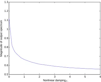
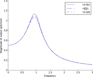
=0.001 =0.01 =0.028
Figure 6. Magnitude characteristics of system output spectrum with respect to frequency ωand different nonlinear damping ξ2 withξ1=0.5
1
ξ
ω
2
ξ
[image:16.595.110.415.422.673.2]0 0.5 1 1.5 2 2.5 3 0
0.2 0.4 0.6 0.8 1 1.2 1.4
Frequency(rad/s)
M
ag
ni
tude
of
ou
tp
ut
s
pe
c
tr
um
[image:17.595.133.449.115.374.2]=0.5 =0 =0.54 =0 =0.5 =0.028
Figure 7. Magnitude characteristics of system output spectrum with respect to frequency ωand different nonlinear damping ξ2 andξ1
0 0.5 1 1.5 2 2.5 3
0 0.2 0.4 0.6 0.8 1 1.2 1.4
Frequency(rad/s)
M
a
gn
it
ud
e o
f ou
tpu
t s
p
ec
tr
um
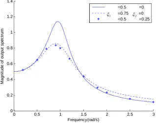
=0.5 =0 =0.75 =0 =0.5 =0.25
Figure 8. Magnitude characteristics of system output spectrum with respect to frequency ωand different nonlinear damping ξ2 andξ1(“*”from simulations)
2
ξ
1
ξ
0.88 0.9 0.92 0.94 0.96 0.98 1 1.02 1.02
1.04 1.06 1.08 1.1 1.12 1.14 1.16
2.48 2.5 2.52 2.54 2.56 2.58 2.6 2.62 0.135
0.14 0.145 0.15 0.155 0.16
1
[image:17.595.133.452.429.681.2]5
Conclusions
The cubic nonlinear damping is studied in the frequency domain through a dimensionless vibration system model actuated by a harmonic input. Theoretical analysis and simulation show that the cubic nonlinearity drives the system output spectrum to be an alternative series at the natural frequency 1, which can be used to suppress the magnitude level of the output spectrum, and the magnitude frequency characteristics of the system output spectrum at higher or lower frequencies than the natural frequency 1 after the cubic nonlinear damping is introduced is very similar to those before the cubic nonlinear damping is introduced. These results can provide a significant insight into the design of active and passive nonlinear vibration systems in practice. Further study will extend these results to a more general case.
Appendix A: Proof of Lemma 1
To compute the GFRFs for system (1), consider a more general model described by the following nonlinear differential equation (NDE)
0 ) ( )
( )
, , (
1 0 , 0 1 1
1 ,
1
=
∑∑ ∑
∏
∏
= = =
+
+ = =
+
+
M
m m
p K
k k
q p
p i
k k p
i k k q p q
p
q p
i i
i i
dt t u d dt
t y d k
k
c L (A1)
where () ()
0
t x dt
t x d
k k k
=
=
, p+q=m,
∑
∑
∑
= =
= +
+
⋅ ⋅
=
⋅ K
k K
k K
k
k, pq 0 0 pq 0
) ( ) ( ) (
1 1
L , M is the maximum degree of nonlinearity in terms of y(t) and u(t), and K is the maximum order of the derivative. It is obvious that model (1a) is just a very special case of model (A1) with c10(0)=1, c10(2)=1,
c10(1)=ξ1, c30(111)=ξ2, c01(0)=-1, K=2, M=3 and all other parameters zero.
For model (A1), the GFRFs can be computed through an algorithm provided in [1]
∑ ∑
∑∑ ∑
∏
∑
= = −
= −
= =
− −
=
+ − +
=
+ +
= ⋅
+ +
+
+
n
p K
k k
n p
n p p
n
q q n
p K
k k
q n p
q n q
i
k i q n q
p q
p
K
k k
k n k n n
n n
n n
p q p
i p n
n
j j H k k c
j j H j
k k c
j j
k k c j
j H j j
L
2 , 0
1 , 1
0 , 1
1 1 , 0
1 , 1
1 ,
0 ,
1 1
, 0 1
1
1 1
1
1
) , , ( ) , , (
) , , ( ) ) ( )( , , (
) ( ) )( , , ( )
, , ( ) (
ω ω
ω ω ω
ω ω
ω ω ω
ω
L L
L L
L L
L L
(A2)
∑
− += − − +
+ + =
⋅ 1
1
1 1
1 , 1
, () ( , , ) ( , , )( )
p n
i
k i n
i p i n i i
p n
p
j j
j j
H j j H
H ω L ω ω L ω ω L ω (A3)
1
) )(
, , ( ) , ,
( 1 1 1
1 ,
k n n
n n
n j j H j j j j
H ω L ω = ω L ω ω +L+ ω (A4) where Ln( jω1+L+ jωn)=
∑
=
+ + − K
k
k n
j j
k c
0
1 1 0 , 1
1
1
) )(
( ω L ω . Moreover, equation (A3) can also be written as
∑ ∏
− + == =+ +
+ +
∑
+ +
= 1
1 1
1 1
1 ,
1
) )(
, , ( )
, , (
p n
n r
r r
p
i
k r r r
r r r
r n
p n
i p
i i X X
i X X
i j j j j
H j
j H
L
L L
L ω ω ω ω ω
ω (A5)
where
∑
−
=
= 1
1
i
x x
To obtain the frequency response functions for the SDOF vibration system (1), the system can be regarded that it has one input u(t) and two outputs x(t) and y(t). The GFRFs for the relationship between y(t) and u(t) are dependent on the GFRFs for the relationship between x(t) and u(t). Therefore, the later are derived first in the following.
By the parametric characteristic analysis in [15], the nth-order GFRF for the relationship between x(t) and u(t) can be expressed as
(
( , , ))
( , , )) , ,
( 1 x 1 n n 1 n
n n
x
n j j CEH j j f j j
H ω L ω = ω L ω ⋅ ω L ω
where fn(jω1,L,jωn)is a complex valued vector, “⊕” and “⊗” are two operators defined
in [15],
(
( 1, , n))
x
n j j
H
CE ω L ω is referred to as the parametric characteristic of the nth-order GFRF
⎣ ⎦
⎟ ⎟ ⎠ ⎞ ⎜
⎜ ⎝ ⎛
⋅ ⊗
⊕ ⊕ ⊕ ⎟ ⎠ ⎞ ⎜
⎝
⎛⊕⊕ ⊗ ⋅ ⊕
= − +
+
= +
− − −
= −
= ( ()) ( ())
)) , , (
( ,0 1
2 1
2 0 , 1
, 1 1
1 , 0 1
x p n p
n
p n x
p q n q
p q n
p n q n n x
n j j C C CE H C C CE H
H
CE ω L ω
According to the results in [17], for model (1)
)) , , ( ( )) , , (
( 1 1 n
x n n
y
n j j CE H j j
H
CE ω L ω = ω L ω
Note also that there is only one nonlinear term with coefficient c3,0(1,1,1), thus it can be obtained that the nth-order GFRF for the relationship between y(t) and u(t) can be expressed as for n=0,1,2,3,…
) , , ( )
, ,
( 1 2 1 2 2 1 1 2 1
1
2 + + = ⋅ n+ n+
n n y
n j j f j j
H ω L ω ξ ω L ω (A6)
0 ) , ,
( 1 2
2 n =
y
n j j
H ω L ω (A7) Hence, only odd order GFRFs need to be computed. From (A2) it can be derived that for the first order GFRF,
) (
1 ) (
1 1 1
1 ω ω
j L j
Hx = − (A8)
and for n=1,2,3,…
0 ) , ,
( 1 2
2n j j n =
H ω L ω (A9)
) (
) , , ( )
, , (
1 2 1
1 2
1 2 1 3 , 1 2 2 1 2 1 1 2
+ +
+ +
+
+ = + +
n n
n n
n x
n
j j
L
j j H j
j H
ω ω
ω ω ξ
ω ω
L L
L (A10)
∑
− =+ +
− +
+ ⋅ = + +
1 2
1
1 1 2 1 2 , 1 2 1
3 , 1
2 () ( , , ) ( , , )( )
n
i
i n
i i n i x
i
n H j j H j j j j
H ω L ω ω L ω ω L ω (A11)
1
) )(
, , ( )
, ,
( 1 2 1 2 1 1 2 1 1 2 1
1 , 1 2
k n n
x n n
n j j H j j j j
H + ω L ω + = + ω L ω + ω +L+ ω + (A12)
L2n+1(jω1+L+ jω2n+1)=
(
)
2 1 2 11 2 1
1( ) ( )
1+ + + + + + + +
− ξ jω L jω n jω L jωn (A13)
From (A5), (A11) can also be written as
∑ ∏
−+ =
= =
+ +
+ +
+ +
∑
+ + =
1 2
1 2 1
3
1
1 1
1 2 1 3 , 1 2
1
) )(
, , ( )
, , (
n
n r r
r i
r X X
r X X
x r n
n
i p
i i
i j j j j
H j
j H
L
L L
L ω ω ω ω ω
ω (A14)
Based on equations (A8-14), the GFRFs for the relationship between y(t) and u(t) can be obtained by applying the results in [17]. For n=0,1,2,3,…
0 ) , ,
( 1 2
2 n =
y
n j j
H ω L ω and
∑ ∑
+
= =
+ +
+
+ =
1 2
1 1
0 ,
1 2 1 , 1 2 1
0 , 1
2 1 1 2
1
) , , ( ) , , ( ~ )
, , (
n
p k k
n p
n p p
n y
n
p
j j H k k c j
j
Noting thatc~1,0(0)=1, 1,0(1) 1
~ =ξ
c , ~c3,0(1,1,1)=ξ2and other parameters of form c~p,0(k1,L,kp)
zero and using (A11), it can be further obtained that for n=0,1,2,3,…
(
1 ( ))
( , , ) ( ( )) ( , , ) ( 15)) , , ( )) ( ( ) ( ) , , ( ) , , ( ) , , ( ) 1 , 1 , 1 ( ~ )) ( ( ) , , ( ) 1 ( ~ ) , , ( ) 0 ( ~ ) , , ( 1 2 1 3 , 1 2 2 1 2 1 1 2 1 2 1 1 1 2 1 3 , 1 2 2 1 2 1 1 2 1 1 2 1 1 2 1 1 2 1 2 1 3 , 1 2 0 , 3 1 2 1 1 , 1 2 0 , 1 1 2 1 1 , 1 2 0 , 1 1 2 1 1 2 A j j H n j j H j j j j H n j j j j H j j H j j H c n j j H c j j H c j j H n n n x n n n n n n x n n x n n n n n n n n y n + + + + + + + + + + + + + + + + + + + + + ⋅ + + ⋅ + = + + + ⋅ + = + + = ω ω ξ δ δ ω ω ω ω ξ ω ω ξ δ δ ω ω ω ω ξ ω ω ω ω δ δ ω ω ω ω ω ω L L L L L L L L L L L where ⎩ ⎨ ⎧ = = else 0 0 1 )
(n n
δ . From (A10) and (A15), it can be obtained that for n>0,
(
)
(
)
) , , ( ) ( ) ( ) , , ( ) ( ) , , ( ) ( 1 ) , , ( ) , , ( ) ( 1 ) , , ( 1 2 1 3 , 1 2 1 2 1 1 2 2 1 2 1 2 1 2 1 3 , 1 2 2 1 2 1 1 2 1 2 1 3 , 1 2 2 1 2 1 1 1 2 1 3 , 1 2 2 1 2 1 1 2 1 2 1 1 1 2 1 1 2 + + + + + + + + + + + + + + + + + + + + + + + − = + + + + + ⋅ + = + ⋅ + + ⋅ + = n n n n n n n n n n n n n n n x n n n y n j j H j j L j j j j H j j L j j H j j j j H j j H j j j j H ω ω ω ω ω ω ξ ω ω ξ ω ω ω ω ξ ω ω ξ ω ω ξ ω ω ω ω ξ ω ω L L L L L L L L L L LUsing (A14) yields for n>0
∑ ∏
− + = = = + + + + + + + + + ∑ + + + + + + −= 2 1
1 2 1 3 1 1 1 1 2 1 1 2 2 1 2 1 2 1 2 1 1 2 1 ) )( , , ( ) ( ) ( ) , , ( n n r r r i r X X r X X x r n n n n y n i p i i
i j j j j
H j j L j j j j H L L L L L L ω ω ω ω ω ω ω ω ξ ω ω (A16)
This completes the proof.
Appendix B: Proof of Lemma 2
When the system input is a multi-tone function described by
∑
= ∠ + = K i i ii t F
F t u 1 ) cos( )
( ω (B1)
the system output frequency response function can be obtained according to [7],
∑
∑
= + + = = N n k k k k n n n k k nn F F
j j H j Y 1 1 1
1, , ) ( ) ( )
( 2 1 ) ( ω ω ω ω ω ω ω ω L L
L (B2)
where
{
}
⎪⎩ ⎪ ⎨ ⎧ ∈ =± ± = ∠ else 0 , , 1 , if )
( F e k K
F k
F j i
i ω ω L
ω and ωk =sign(k)ω|k|.
Using the GFRFs determined by equations (4-8) for the relationship from u(t) to y(t), the system output spectrum can then be determined by substituting (8) in (B2) gives
⎣ ⎦ ⎣ ⎦
∑
∑
∑
∑
− = + + = + + − = + + + = + + + + + + + = = 2 1 0 1 2 1 2 2 2 1 0 1 2 1 2 1 2 1 1 2 1 1 2 1 1 2 1 1 2 1 1 2 1 ) ( ) ( ) , , ( 2 ) ( ) ( ) , , ( 2 1 ) ( N n k k k k n n n N n k k k k y n n n k k n n n k k n n F F j j f F F j j H j Y ω ω ω ω ω ω ω ω ω ω ξ ω ω ω ω ω L L L L L L (B3)For the specific input function (1b), it can be obtained from (B2) that
d l k jkF
F
l)=−