Monte Carlo comparison of back-propagation, conjugate-gradient, and finite-difference training algorithms for multilayer perceptrons

Rochester Institute of Technology

RIT Scholar Works

Theses Thesis/Dissertation Collections

2011

Monte Carlo comparison of back-propagation,

conjugate-gradient, and finite-difference training

algorithms for multilayer perceptrons

Stephen Wehry

Follow this and additional works at:http://scholarworks.rit.edu/theses

This Dissertation is brought to you for free and open access by the Thesis/Dissertation Collections at RIT Scholar Works. It has been accepted for inclusion in Theses by an authorized administrator of RIT Scholar Works. For more information, please [email protected]. Recommended Citation

Monte Carlo Comparison of Back-Propagation,

Conjugate-Gradient, and Finite-Difference

Training Algorithms for Multilayer Perceptrons

By Stephen J. Wehry

A Dissertation fulfillment of the requirements for the Master’s

Degree in Mathematics

Thesis Adviser: Dr. Alejandro Engel

Rochester Institute of Technology

Department of Mathematics and Statistics

MASTER’S DISSERTATION

OF

STEPHEN JOSEPH WEHRY

April, 7, 2011

APPROVED:

Dissertation Committee:

Major Professor ____________________________

Dr. Alejandro Engel

____________________________

Dr. James Marengo

____________________________

Dr. Michael Radin

Table of Contents

ABSTRACT ... 4

INTRODUCTION ... 5

TEST PROBLEMS AND ENCODING SCHEMES ... 9

PRECISION TEST - PATTERN RECOGNITION ... 9

GENERALIZATION TEST - BIT COUNTING ... 10

HEURISTICS USED ... 10

EXAMPLE MULTILAYER PERCEPTRON – “XOR” FUNCTION ... 12

TRAINING ALGORITHMS TESTED ... 16

THE BACK-PROPAGATION ALGORITHM ... 16

THE CONJUGATE-GRADIENT ALGORITHM ... 21

THE FINITE-DIFFERENCE ALGORITHM ... 26

MONTE CARLO SIMULATION ... 28

TEST METHODOLOGY ... 28

SIMULATION RESULTS ... 29

A Note About ρ Values ... 29

Pattern Recognition ... 29

Bit Counting ... 31

CONCLUSIONS AND FUTURE WORK ... 37

REFERENCES ... 39

APPENDICES ... 40

APPENDIX A: PATTERN RECOGNITION CALCULATOR DIGITS ... 40

APPENDIX B: BIT COUNTING TRAINING EXAMPLE SET ... 41

APPENDIX C: DERIVATION RESULTINGFROM HIGHER-ORDERΡ VALUES ... 42

APPENDIX D: RAW MONTE CARLO SIMULATION DATA ... 43

D1: Back-Prop Pattern Recognition ... 43

D2: C-G Pattern Recognition ... 47

D3: Finite-Difference Pattern Recognition ... 54

D4: Back-Prop Bit Counting ... 58

D5: C-G Bit Counting ... 71

Abstract

Monte Carlo Simulation is used to compare the performance of the

Introduction

Multilayer perceptrons (hereafter denoted as MLPs) are a well-studied type of

neural network, dating back to the pioneering work of Rosenblatt in 19581._{. This paper}

describes a comparison of three training methods, back-propagation,

conjugate-gradient, and finite-difference algorithms, used to train simple MLPs to solve each of two different problems: pattern recognition and bit counting. Each of these training

methods follow the supervised learning paradigm2. _{in which training examples are}

presented from which an error signal is generated. This error signal is then used to train

the network to learn to solve the problem at hand in different (but related) ways. All of the MLPs used in this paper have the same general structure depicted in Figure 1 below.

Figure 1: 3-Layer Fully-Connected MLP Topology

Each MLP in this study consists of three layers, one input layer, one hidden

solved; the number of hidden neurons was varied as part of this study. All of the networks used in this paper have the following properties in addition to those already mentioned:

• They are fully-connected, meaning that each neuron in both the input and hidden

layers is connected to every neuron in the subsequent layer3._.

• They are feed-forward, meaning that during computation information flows in one

direction from the input, through the hidden, and ending in the output layer. This

means that there is no use of online feedback4._{. An additional constraint on the}

topology of the networks in this study is that there is no skipping of layers.

• All non-input neurons utilize a nonlinear activation function5._.

• Input neurons are for input only, hidden neurons are for computation only, and output

neurons are for computation and output. In this context computation means the

process of summation of the input signals to an individual neuron then the application of the activation function.

Figure 2: Computational Structure of Input Node i

The function of an input node is to receive its single input signal and pass it on to each

neuron in the hidden layer after applying the appropriate synaptic weight6. _{for that}

connection.

Figure 3: Computational Structure of Hidden Node j

Figure 3 shows that a hidden node first sums up its inputs from the previous layer, adds its bias, then applies the activation function to this value. The resulting value is then passed on to become part of the input of each neuron in the output layer, again, after the

appropriate synaptic weight has been applied7._.

The computational structure of the kth output neuron is shown below in Figure 4.

An output neuron acts just like a hidden neuron, except that no weight is applied to the output of the activation function in these nodes8._.

Finally, consider a few miscellaneous notes on the overall properties of the network. First, the functional form and parameters of φ(x) were heuristically chosen for two main reasons. A sigmoid function, such as the hyperbolic tangent function used in this study, has the necessary properties of nonlinearity, monotonicity, antisymmetricity, and range-boundedness. The parameters were chosen to maximize the curvature of this function at x = y = + 1, which helps to prevent neurons from being driven to saturation, a serious obstacle to the convergence of the training algorithm. This leads to the second general property of the networks used, which is that both the input and output spaces of each problem are encoded into vectors x with -1 < xi < 19..

Test Problems and Encoding Schemes

Precision Test - Pattern Recognition

The pattern recognition problem used in this study is for the MLP to correctly identify ten simple five-by-three pixel calculator digits detailed in Appendix A. To illustrate the input space encoding scheme, consider the fifteen pixel calculator digit for zero, shown below in Figure 5.

Figure 5: Pattern Recognition Input Space Encoding Scheme

[1, 0, 0, 1], and so on. Finally, the network will be presented with one example of each of the ten digits during each epoch of training.

Pattern Recognition is a so-called precision test because there are a small number of possible inputs, meaning that all of them can be presented to the network during each training epoch. This means that since no generalization outside of the training space will be required, the network’s only task is to learn these examples to a high degree of accuracy.

Generalization Test - Bit Counting

The bit counting problem used in this study is to have the network count the number of “1”s in an arbitrary binary string seven bits long. Naturally the input space for this problem will consist of vectors with seven components. The output space of the network will be a binary representation of the numeric value of the answer. Since there are a maximum of seven “1”s in a seven bit string, the output space will be a vector with three components.

In this study there are 27 _{= 128 possible input strings, but only a subset of 68 them}

will be used as training examples. Since the network will be tested against each of the 128 possible inputs, this test presents the network an additional challenge, that of generalization from the known to the unknown.

Heuristics Used

Several heuristics for improving the performance of MLPs have grown out of the cumulative work that has been done over the years since their introduction. Many have been incorporated into and used in this study; they are listed below.

• Pre-processing of input and output spaces – Remove the mean of each to ensure

that the components of the input and output vectors are not all positive or all negative10._.

• “Euclidean Distance Output” calculation – both pattern recognition and bit

Euclidean-distance sense. That closest valid output vector is what is used as the reported output of the network.

• Synaptic weight initialization - Calculate initial values for synaptic weights

according to a uniform distribution function; use layer size to determine variance of same11._.

• In the Back-Prop Algorithm, each synaptic weight has its own individually

Example Multilayer Perceptron – “XOR” Function

As an illustrative example of using an MLP is to consider the MLP diagrammed below in Figure 6, designed to solve the “Exclusive Or”, or “XOR” problem.

Figure 6: “XOR” MLP Schematic

The XOR function, of course, gives values according to the following truth table.

Input 0 Input 1 Output Value

0 0 0

1 0 1

0 1 1

1 1 0

Table 1: “XOR” Truth Table

Parameter Value After Successful Training Whidden,0,0 0.362985

Whidden,0,1 0.418378

Whidden,1,0 -0.464486

Whidden,1,1 -0.554121

Whidden,2,0 -0.720958

Whidden,2,1 0.504430

Woutput,0,0 0.620124

Woutput,1,0 -0.446396

Woutput,2,0 0.692502

Table 2: Example MLP “Trained” Parameter Values

Following the heuristics described in the previous section, the first step in using this example MLP is to pre-process the input values by subtracting out the mean of the input space. The four possible input vectors in the “XOR” problem are (0,0), (1,0), (0,1), and (1,1). The mean value of the first component of the possible input space is (0+1+0+1) / 4 = 0.5, and that of the second component is also (0+0+1+1) / 4 = 0.5. Therefore before we present the network with an input, we first subtract the vector (0.5, 0.5), resulting in the following table of possible pre-processed input values.

Original Input Vector

Pre-Processed Input Vector (Zero-Mean)

(0, 0) (-0.5, -0.5)

(1, 0) (0.5, -0.5)

(0, 1) (-0.5, 0.5)

(1, 1) (0.5, 0.5)

Table 3: Example MLP Zero-Mean Input Values

Figure 7: “XOR” MLP Calculation: Input Layer

Now the values of the hidden layer neurons must be calculated, using the values of the input layer along with the synaptic weights and biases that are shown in Figure 7.

{

}

0 (i )(Whidden ) (i )(Whidden ) bhidden

h = ϕ  +  + 

{

}

0 = ϕ + − + −

h

(

)

tanh 7159 . 1 ) 771709 .

0

( ₃2

0 = ϕ − = − = −

h

Similarly,

{

}

1 (i )(Whidden ) (i )(Whidden ) bhidden

h = ϕ  +  + 

{

}

1 = ϕ + − +

h

(

)

7159 . 1 ) 436559 .

0

( ₃2

1 = ϕ = =

h ,

Figure 8: “XOR” MLP Calculation: Hidden Layer

The next step is to calculate the value of the output neuron:

{

}

0 (h )(Woutput ) (h )(Woutput ) boutput

o = ϕ  +  + 

{

}

0 = ϕ − + − +

o

(

)

tanh 7159 . 1 ) 028092 .

0

( ₃2

0 = ϕ − = − = −

o ,

which results in the final network state shown in Figure 9.

The calculated output of the example MLP to the input (1, 1) is -0.032132, but the possible outputs of the actual “XOR” problem are restricted to either 1 or 0. This is because this MLP was trained using zero-mean output values (another of the heuristics listed in the previous section), which are tabulated below in Table 4.

Original

Output Vector Output VectorZero-Mean

(0) (-0.5)

(1) (0.5)

Table 4: Example MLP Zero-Mean Output Values

So, the possible zero-mean output values for the “XOR” problem are -0.5 or 0.5 – to which does the output value -0.032132 of our example MLP correspond? This final step in the MLP calculation involves computing the Euclidean distance of our output vector to each of the possible zero-mean output vectors, and choosing that which is closest. We calculate

[

]

5 . 0 ( ) 032132 .

0

(− − = − − 2 =

[

]

5 . 0 ( ) 032132 .

0

(− − − = − − − 2 = ,

so the final output of the example MLP to the “XOR” of (1, 1) is 0.

Training Algorithms Tested

As mentioned in the Introduction, both training methods used in this study employ the supervised learning paradigm, in which adjustments are made to the network’s

parameters due to errors in the output response to training examples13._{. However, even}

small MLPs like those in this study have a large number of such parameters in the form of synaptic weights between and biases of their neurons. Which parameters should be

adjusted when, and by how much, during training? This is what is known as the “credit

assignment problem” for MLPs that training algorithms are designed to solve14._.

The Back-Propagation Algorithm

One of the first computationally efficient solutions to the credit assignment problem, and still one of the most powerful and popular neural network training

algorithms, is the back-propagation (back-prop) algorithm15._{. Back-propagation is}

Rule of Calculus to propagate the error signal of each training example back,

layer-by-layer, through the network. Hebbian Learning adjustments are made to the parameters

of each layer in proportion to the contribution of each individual parameter to the overall error signal16._.

The back-prop formulas are derived as follows. First, assume an MLP with N

input, M hidden, and P output neurons. Let d be the vector (dimension P) of desired

response for the training example presented to the network as input vector i (dimension

N). Given the current state of the network (i.e., the values of the weight and bias

parameters for each neuron), the network will calculate an output response vector o

(dimension P), the vector of the output values of the output neurons. The output values will differ from the desired response by an amount

k k k d o

e =  −  , k = 1, …., P (1.)

for each output neuron k. This value is the error signal for the kth neuron in response to the current training example. An energy-like total error in response to the current training example can be computed as

∑

∑

= =

= −

= P

k k P

k

k

k o e

d E

1 2 2

1

1

2 2

1 ₍  _{) (} _{) . (2.)}

This is the error signal that will be propagated back through the network to effect training. Using the Hebbian Learning analogy, we wish to adjust each parameter by an amount proportional to its individual contribution to this total error, as in

        ∂

∂ − = ∆

ij ij

W E

W λ , (3.)

where the value λ is the called the learning rate parameter. The following derivation17.

provides a value for

ij

W E ∂

∂

.

= 0 to N, where y0= 1 is the “signal” which, when multiplied by the bias value bj = W0j,

gives the bias term of the calculation. Let Wij be the matrix of synaptic weights from the

previous layer to the layer containing neuron j. The value

∑

=

= N

i

i ij

j W y

v 0

) )(

( 



(4.)

is called the induced local field of neuron j. The output signal of neuron j in response to the current training example is

) ( _j

j v

y = ϕ  . (5.)

Now, using the Chain Rule of Calculus,

ij j

j j

j j

j

ij W

v v y y e e

E W

E

∂ ∂ ∂ ∂ ∂ ∂ ∂

∂ = ∂

∂ 

   

 , (6.)

which gives an expression for the value we want in terms of values we can calculate. First, differentiate equation (2.) to get

j j

e e

E 

 =

∂ ∂

. (7.)

Recall that for non-input neuron j,

j j j d y

e =  −  , (8.)

from which we get, via differentiation,

1

− = ∂ ∂

j j

y e

 

. (9.)

To get the fourth factor of the right side of equation (6.), we differentiate equation (5.) to get

) ( _j

j j

v v

y 

 

ϕ ′ = ∂ ∂

. (10.)

Finally, by differentiating equation (4.) we get

i ij j

y W

v ₌  ∂

∂

. (11.)

] )][ ( ][

[ _{j j i}

ij

y v e

W

E   

ϕ ′ − = ∂

∂

, (12.)

which gives the following expression for equation (3.): ] )][ ( ][

[ _{j j i}

ij e v y

W = λ  ϕ′  

∆ . (13.)

The value [ej][ (vj)]

 

ϕ ′ is denoted by δ j



and is called the local gradient of neuron j.

Note that if neuron j is an output node equation (12.) is readily evaluated, but due

to the presence of the desired response in ej



, further calculation to define this value is

necessary in the case where neuron j is a hidden neuron. The local gradient δ j



is defined

as

j j

j j

v E v

e  



∂ ∂ − = ′

= [ ][ϕ ( )]

δ (14.)

j j

j v

y y

E

  

∂ ∂ ∂

∂ −

= (15.)

) ( _j

j

v y

E 

 ϕ ′ ∂

∂ −

= _{, (16.)}

where the Chain Rule is used in equation (15.). Following Haykin (1999), note that in equation (2.) the summation is over the output nodes k. Differentiating equation (2.) yields

∑

= 

   

  

∂ ∂ =

∂

∂ P

k j

k k

j y

e e y

E

1

  

 . (17.)

Again the chain rule is used to get

∑

= 

   

  

∂ ∂ ∂ ∂ =

∂

∂ P

k j

k

k k k

j y

v v e e y

E

1

    

 . (18.)

Since neuron k is an output neuron, recall from equation (8.) that

k k k d y

e =  −  (8.)

). ( _k

k v

d − ϕ 

= (19.)

) ( _k

k

k _v

v

e 

 

ϕ ′ − = ∂ ∂

(20.)

Using equation (4.) we can write the induced local field of neuron k as

(

)

∑

=

= M

j

j jk

k W y

v 0

] ][

[ 



, (21.)

so we get that

jk j k _W

y v

= ∂ ∂  

. (22.)

Finally, plugging the two partials (20.) and (22.) back into equation (18.) yields

(

)

∑

=

′ −

= ∂

∂ P

k

jk k k

j

W v e y

E

1

] )][ ( ][

[ 

 ϕ (23.)

and

(

)

∑

=

− = ∂

∂ P

k k jk j

W y

E

1

] ][ [δ

 . (24.)

Plugging equation (24.) into equation (15.) yields what is known as the

back-propagation formula,

∑

=

′

= P

k

jk k j

j v W

1

) ( )

( δ

ϕ

δ   (25.)

for hidden neuron j. This provides the algorithmic mechanism to calculate the “local contribution” of hidden neuron j to the overall error signal for the current training example18._.

Line # 3-Layer MLP with N input, M hidden, and P output neurons Comments 1 Initialize epoch counter = 0

2 Initialize (M+1 by P) output layer weights matrix Woutput Uniform Distribution with μ = 0, σ2 = 1 / M

3 Initialize (M+1 by P) output layer learning rate matrix λoutput Use an initial value of 0.01

4 Initialize (N+1 by M) hidden layer weights matrix Whidden Uniform Distribution with μ = 0, σ2 = 1 / N

5 Initialize (N+1 by M) hidden layer learning rate matrix λhidden Use an initial value of 0.01

6 While not done training do 7 For x = 0 to NUM_EXAMPLES 8 Set input vector i = training example x 9 Set desired response vector d

10 Compute hidden layer vector h See Figure 3 above. 11 Compute output layer vector o See Figure 4 above.

12 Compute error signal component Ex

∑

= −

= P

i i i

x d o

E

1 2 2

1 ₍ ₎

13 Calculate output layer local gradient vector δoutput _{v d o k P}

k k k output k

output, = ′( , )( − ); =1...

   

ϕ δ

14 Calculate hidden layer local gradients vector δhidden

M j W

v P

k

k j output k output j

hidden j

hidden ( ) ( ); 1...

1

, , , ,

, = ′ ∑ =

=

δ ϕ

δ  

15 Adjust output layer weights matrix Woutput _{W W h j M k P}

j k output k j previous k j output k j

output,. = ( ,.) +( ,)( ,)( ); =1... ; =1... 



δ λ

16 Adjust hidden layer weights matrix Whidden _{W W i i N j M}

i j hidden j i previous j i hidden j i

hidden,. = ( ,.) +( ,)( ,)( ); =1... ; =1... 



δ λ

17 Adjust individual learning rates matrices λhidden, λoutput

18 Next x

19 Calculate Average Error Value Eavg

( ) E NE NUM EXAMPLES

E NE

x x NE

avg , _

1

1 ₌

   

= ∑

=

20 If stopping criteria is not met Then increment epoch count Else done training is true

21 Loop back to line 4

22 Record # epochs, total training time, initial average error, and final average error

23 STOP

Table 5: The Back-Propagation Algorithm

The Conjugate-Gradient Algorithm

The method of conjugate gradients is an algorithm for exactly minimizing the

quadratic vector equation ½(xT_{Ax) – bx + c= 0, when the n-by-n matrix A is}

positive-definite19._{. This algorithm adjusts the n-by-1 vector x to minimize the equation along each}

of a constructed sequence of n A-conjugate vectors, the resulting value of x being the

desired minimizing value. If the matrix A is known and positive-definite the sequence of

A-conjugate vectors can be directly calculated and the algorithm finishes in at most n

steps.

To begin our discussion of this algorithm, we must define the concept of A

-conjugacy. A non-zero set of N vectors {s0, s1, s2,…, sN-1}is called A-conjugate with

respect to the N-by-N positive definite matrix A if

j i s A

sT _j

i = 0, ≠

 

The concept of A-conjugacy is a generalization of the more commonly used idea of

orthogonality of vectors. Like a set of mutually orthogonal vectors, a set of A-conjugate

vectors is linearly independent. This can be proven by contradiction as follows. Without

loss of generality, assume we have the A-conjugate set {si}, i=0,…,N-1, and assume that

∑

=

= 1

1 0

N

j j js

a

s 



(27.)

in other words, that the set of vectors is linearly dependent. Left-multiply Equation (27.) by the matrix A to get

∑

=

= 1

1 0

N

j

j jAs

a s

A  _{. (28.)}

Again left-multiply by s₀T to get

∑

=

= 1

1 0 0

0

N

j

j T j T_{As a s As}

s    _{, (29.)}

but because we assumed that the set {si}was A-conjugate, the right side of Equation (29.)

is zero, so we see that

0

0 0 As = sT 



. (30.)

This is our contradiction because by definition s0 is nonzero and the matrix A is

positive-definite, therefore the set of A-conjugate vectors must be linearly independent20._.

The conjugate-gradients algorithm can be adapted for use in a generic nonlinear minimization problem due to the theoretical fact that any function can be Taylor

expanded to “look” like a second-order system in the neighborhood of a local minimum. The training of an MLP can be considered as such a problem, where the average squared error over a training epoch is used as the nonlinear function to be minimized. In the neighborhood of a local minimum, the error surface is described by

c w b w A w w

E T T

Avg ≈ − +

    

2 1

)

( . (31.)

Clearly in the general neural network application the matrix A, the vector b, and the

scalar c are unknown, so we develop a method to calculate the sequence of A-conjugate

Given the situation in Equation (31.), the idea behind conjugate-gradients is to generate a sequence of A-conjugate search vectors s0, s1, s2,…, sN-1 to adjust the parameter

vector w using the update equation

n n

n w s

w ₊1 =  + η , n=0,…,N-1, (32.)

where the scalar η is defined as the value that minimizes the value of EAvg(wn sn)

 

η +

when both wn and snare held constant. First, define the residual vector

n

w w Avg n

n

w w E w

A b r

 

  

 

=

∂ ∂ = −

= ( ) , (33.)

the gradient vector of the error surface evaluated at the current point w on the error

surface.

We begin the algorithm by choosing an arbitrary initial value of w0, and setting

our initial search vector

0

) (

0 0

w w Avg o

w w E w A b r s

 

  

  

=

∂ ∂ = − =

= _{. (34.)}

We’ll use the conjugate Gram-Schmidt22. _{procedure to construct the remaining search}

vectors such that

∑

=

+

= 1

0

i

k k ik i

i r s

s  



β . (35.)

Take the inner product of Equation (35.) with the vector Asj, 0 < j < i, to get

) ( )

( )

( 1

0 j

i

k ik k i

j

i As r s As

s ⋅  = _ +

∑

=

β (36.)

[

]

∑

=

⋅ +

⋅ =

⋅ 1

0

) ( ) ( )

( ) ( ) ( )

( i

k ik k j j

i j

i As r As s As

s    β   (37.)

[

]

∑

=

+

= 1

0

i

k

j T k ik j

T i j T

i As r As s As

s     



β . (38.)

Recall that the set {si} is A-conjugate, so

j i s A

sT _j

i = 0, ≠

 

, (39.)

so

j j ij j T

i As s As

r  + β  

=

and solving Equation (40.) for βij gives

j T j

j T i ij

s A s

s A r

 

  − =

β . (41.)

However, we want to be able to compute βij without explicitly using or even knowing the

matrix A, so we must continue our calculation. From the method of steepest descent we

know that the residual vectors we have defined are related by the recurrence relation

i i i

i r As

r₊₁ =  − α  . (42.)

Taking the inner product

) ( ) ( ) ( ) ( ) ( )

(r_i ⋅ r_j+1 = r_i ⋅ r_j − α _j r_i ⋅ As_j (43.)

j T i j j T i j T

i r r r r As

r ₊1 =   − α   (44.)

and rearranging Equation (44.) yields

1 +

−

= j

T i j T i j T i

jr As r r r r

     

α , (45.)

and therefore











+

=

−

=

=

otherwise

j

i

r

r

j

i

r

r

s

A

r

i i T i

j T

i _i

i

,

0

1

,

,

1

1 1













α α

. (46.)

Plugging Equation (46.) into Equation (41.) gives

       

+ >

+ = 

  

= − − −

1 ,

0

1 ,

1

1 1 1

j i

j i s A s

r r

i T i

i T i

i ij

 

 

α

β (47.)

The parameter αi-1 is the steepest descent parameter

1 1

1 1 1

− −

− −

− =

i T i

i T i i

s A s

r s

 

 

α , (48.)

and

1 1

1 1

1

1

− −

− −

−

=

i T i

i T i

i s r

s A s

 

 

α . (49.)

  

   

 =

− − −

− − −

1 1 1

1 1 1

i T i

i T i

i T i

i T i i

s A s

r r r

s s A s

 

  

  

β (50.)

1 1 − −

=

i T i

i T i i

r s

r r

 

 

β , (51.)

where we drop the j subscript from β as it is no longer necessary. We then take the inner

product of the conjugate Gram-Schmidt Equation (35.) with rj to get

) ( )

( )

( 1

0

j i

k k ik i

j

i r r s r

s ⋅  = _ +

∑

=

β (52.)

∑

=

+

= 1

0

i

k

j T k ik j

T i j T

i r r r s r

s     



β , (53.)

and when i = j,

∑

=

+

= 1

0

i

k i

T k ik i

T i i T

i r r r s r

s     



β . (54.)

However, we know that

i k r sT _i

k = 0, <

 

, (55.)

which is the case with each term in the summation in Equation (54.), so

i T i i T

i r r r

s  =  . (56.)

At long last, substitution of Equation (56.) into Equation (51.) gives what is known as the

Fletcher-Reeves equation,

1 1 − −

=

i T i

i T i i

r r

r r

 

 

β . (57.)

This is the equation that, when used in Equation (35.), allows the calculation of the A

-conjugate search vectors {si} using only the values of the residual vectors23..

Practical results have shown that a modification of the Fletcher-Reeves formula is

more effective in the general case. This is called the Polak-Ribiere formula24._{, and is}

given by

(

)

   

   − =

− −

−

1 1

1

, 0 max

i T i

i i T i i

r r

r r r

 

  

β . (58.)

The reason is that the generated search vectors {si} are only perfectly A-conjugate when

values of w far from a local minimum, this tends not to be the case. For this reason the generated sequence of search vectors to “lose conjugacy”, which means they are no longer linearly independent, and thus the search can get “stuck” and fail to converge to a minimum. The Polak-Ribiere formula avoids this pitfall by periodically “resetting” the

conjugate-gradients search at the current value of w by setting the adjustment term βi to

zero, which means the gradient is once again used as the search vector (recall that this is how the conjugate-gradients algorithm starts in the first place)25._.

A summary of the conjugate-gradients algorithm that was used in this paper is shown below in Table 6.

Line # 3-Layer MLP with N input, M hidden, and P output neurons Comments 1 Initialize epoch counter = 0

2 Initialize the weights vector w Uniform Distribution with μ = 0, σ2 _{= 1 / M}

3 Set Initial Learning Rate η=0.10; Annealing Rate ηrate=0.9

4 Set stopping criteria α=0.001

5 Calculate initial vectors g, s, and r0 All three have dimension [M*(N + P) + M + P]

6 While not done training do

7 Use Brent’s Method to calculate value of η which 8 Minimizes EAvg(w+ηs) where w and s are held constant

9 Update weight vector w + w + ηs

10 Use Back-Prop to calculate new gradient vector g

Set rprev= r

11 Set r = -g

12 Use Polack-Ribiere formula to calculate β

(

)

   

    − =

prev T prev

prev T

r r

r r r

 

   , 0 max β

13 Calculate new s = r + βs

14 If stopping criteria is not met Then increment epoch count Stopping criterion met when all training examples have been learned with 100% accuracy.

15 Else done training is true 16 Loop back to Line 6

17 Record # epochs, total training time, initial average error, final

average error, and percent correct Percent Correct is calculated after training time is computed. It is the number of correct answers in a test of all 128 possible input values.

18 STOP

Table 6: The Conjugate-Gradient Algorithm

The Finite-Difference Algorithm

The third training algorithm that will be tested in this study is the so-called

finite-difference algorithm. This algorithm is identical to back-prop except for the computation of gradients during the back-propagation phase. Instead of using the local gradient

calculations in equations (12.), (14.), and (25.), this algorithm will directly calculate the central-difference approximation to each gradient with respect to each weight in the network. Thus, for the finite-difference approximation algorithm,

ε ε ε

2 ) ( )

( + − −

= ∂

∂ EWij EWij

ij

W E

where E(Wij) is the calculated error value, averaged over a training epoch, at that

particular value of the individual weight Wij. The strategic motivation for this algorithm is

to utilize a multiprocessor computer to calculate each central-difference in parallel. This study, however, uses an implementation coded for a single process on a single processing BUS, so the potential for productivity gains through parallel computation are

immediately forfeit. However, since we are interested in testing only accuracy,

generalization ability, and number of training iterations, this study will still be a valid test of the performance of the finite-difference algorithm relative to the other two. A summary of the finite-difference algorithm used in this study is shown below in Table 7.

Line # 3-Layer MLP with N input, M hidden, and P output neurons Comments 1 Initialize epoch counter = 0

2 Initialize (M+1 by P) output layer weights matrix Woutput Uniform Distribution with μ = 0, σ2 = 1 / M

3 Initialize (M+1 by P) output layer learning rate matrix λoutput Use an initial value of 0.01

4 Initialize (N+1 by M) hidden layer weights matrix Whidden Uniform Distribution with μ = 0, σ2 = 1 / N

5 Initialize (N+1 by M) hidden layer learning rate matrix λhidden Use an initial value of 0.01

6 While not done training do 7 For x = 0 to NUM_EXAMPLES 8 Set input vector i = training example x 9 Set desired response vector d

10 Compute hidden layer vector h See Figure 3 above. 11 Compute output layer vector o See Figure 4 above.

12 Compute error signal component Ex

∑ =

− = P

i i i

x d o

E

1 2 2

1 ₍ ₎

13 Calculate output layer central-difference gradients

0001 . 0 ; , , 2

) ( ) (

= ∀ =

∂

∂ + − −

ε

ε ε

ε _{i j}

W

E EWij EWij

ij

15 Adjust output layer weights matrix Woutput _{W W h j M k P}

j k output k j previous k j output k j

output,. = ( ,.) +( ,)( ,)( ); =1... ; =1... 



δ λ

16 Adjust hidden layer weights matrix Whidden _{W W i i N j M}

i j hidden j i previous j i hidden j i

hidden,. = ( ,.) +( ,)( ,)( ); =1... ; =1... 



δ λ

17 Adjust individual learning rates matrices λhidden, λoutput

18 Next x

19 Calculate Average Error Value Eavg

( ) E NE NUM EXAMPLES

E NE

x x NE

avg , _

1

1 ₌

   

= ∑

=

20 If stopping criteria is not met Then increment epoch count Else done training is true

21 Loop back to line 4

22 Record # epochs, total training time, initial average error, and final average error

23 STOP

Monte Carlo Simulation

Test Methodology

The Monte Carlo Simulation designed to test the effectiveness of the three training algorithms is outlined in Table 8, below.

Simulation # (*)

ρ Values (**) Hidden Layer

Size (***)

Test Problem Training

Algorithm

1-12 2, 4, 6 4, 10, 15, 20 Pattern Recog. Back-Prop

13-24 2, 4, 6 4, 10, 15, 20 Pattern Recog. C-G

25-36 2, 4, 6 4, 10, 15, 20 Pattern Recog. Finite-Diff.

37-48 2, 4, 6 4, 6, 8, 10 Bit Counting Back-Prop

49-60 2, 4, 6 4, 6, 8, 10 Bit Counting C-G

61-72 2, 4, 6 4, 6, 8, 10 Bit Counting Finite-Diff.

(*) Each individual simulation in this study is composed of 500 trials. A single trial in this study is defined as one complete run through the training algorithms outlined in Table 1, Table 2, or Table 3.

(**) “ρ” is the exponent of the energy-like error function E to be minimized during training. See Appendix C.

(***) Both the hidden layer size and ρ value were varied in this study, but held constant

during an individual simulation. For example, a Hidden Layer Size of 10 means that

there were 10 neurons in the hidden layer during that simulation.

Table 8: Monte Carlo Simulation Outline

As shown in Table 8, both the size of the hidden layer and the exponent ρ of the energy-like error function E were varied to determine the best value of each to use when comparing the three training algorithms for each problem. See Appendix C for the changes to the preceding training algorithm equations that result from a ρ value greater than 2.

The randomly-generated, uniformly-distributed initial values of the synaptic weights were the random elements in each trial of a given simulation. The effectiveness of the training algorithms in each case was determined by using the data to answer two basic questions:

1. Did the network learn the problem sufficiently well? 2. How much work was required to complete the training?

For each trial in this study, the following was used as the stopping criteria for all

of the three training algorithms tested. The supervised-training trial was said to converge

recognition, 128 for bit counting) in a given epoch. If the network's performance in the training example set was less than 100%, training continues epoch-by-epoch until either convergence or the hard limit of maximum epochs was reached. This hard limit,

determined by empirical testing, was chosen to be 5,000 epochs for pattern recognition and 15,000 epochs for bit counting.

Finally, each of the simulations described above were performed on a Compaq Presario F700 laptop computer with a 1.90GHz AMD Athlon Dual-Core Processor and 2.00GB of RAM.

Simulation Results

A Note About ρ Values

The purpose of this study was to test the most competitive network configurations for each problem-training algorithm combination. In every problem-training algorithm combination in this study the best performance was achieved with a ρ value of 2. In most cases the networks using higher values of ρ performed substantially worse, especially with respect to convergence. It was therefore decided to omit discussion of ρ values greater than 2 from the following discussion, although the relevant performance data for these omitted trials can still be found in Appendix D.

Pattern Recognition

1. Did the network learn the problem sufficiently well?

Algorithm Hidden Layer Size Total Trials Convergent Trials

Back-Propagation 4 500 500

Back-Propagation 10 500 500

Back-Propagation 15 500 500

Back-Propagation 20 500 500

Conjugate-Gradient 4 500 499

Conjugate-Gradient 10 500 500

Conjugate-Gradient 15 500 500

Conjugate-Gradient 20 500 499

Finite-Difference 4 500 500

Finite-Difference 10 500 500

Finite-Difference 15 500 500

Finite-Difference 20 500 500

Table 9: Pattern Recognition Convergence Results

As Table 9 shows, only 2 out of the 6,000 total pattern recognition trials failed to converge, both with the conjugate-gradient method. These two trials do not affect the overall message of Table 9, however, which is that the network was able to learn this problem equally well in all four configurations with each of the three training algorithms.

2. How much work was required to complete the training?

The work required to train the network was measured by the number of epochs necessary to train the network to convergence. The summary statistics for each of the twelve distributions generated in this study are shown below in Table 10.

Algorithm Hidden Layer Size Min.

Epochs Mean Epochs

Median Epochs

Max. Epochs

StDev Epochs

Back-Propagation 4 42 174 66 436 70

Back-Propagation 10 30 93 160 224 31

Back-Propagation 15 12 79 89 186 26

Back-Propagation 20 22 69 76 145 21

Conjugate-Gradient 4 (*) 4 14 14 35 4

Conjugate-Gradient 10 4 9 9 24 2

Conjugate-Gradient 15 3 8 8 24 2

Conjugate-Gradient 20 (*) 3 7 7 20 2

Finite-Difference 4 32 105 98 411 44

Finite-Difference 10 19 61 57 177 22

Finite-Difference 15 13 53 51 142 17

Finite-Difference 20 16 48 45 142 15

(*) Only the 499 convergent trials were used to calculate these summary statistics.

Table 10 shows that the conjugate-gradient algorithm was by far the most efficient in terms of number of epochs required to learn the pattern recognition problem. Among the conjugate-gradient results Table 10 shows that a hidden layer of 20 neurons was the best performing of the configurations tested.

Bit Counting

1. Did the network learn the problem sufficiently well?

In the bit counting problem, the stopping criteria for each training algorithm was the same as in pattern recognition – stop training when the network achieves 100% accuracy across the training set or the hard limit in epochs is reached. Table 11 below is a summary of the convergence results for the bit counting trials (all ρ = 2) performed in this study.

Algorithm Hidden Layer Size Total Trials Convergent Trials

Back-Propagation 4 500 328

Back-Propagation 6 500 471

Back-Propagation 8 500 500

Back-Propagation 10 500 500

Conjugate-Gradient 4 500 347

Conjugate-Gradient 6 500 476

Conjugate-Gradient 8 500 499

Conjugate-Gradient 10 500 500

Finite-Difference 4 500 21

Finite-Difference 6 500 250

Finite-Difference 8 500 413

Finite-Difference 10 500 484

Table 11: Bit Counting Convergence Results

Figure 10: Percent Convergent Trials by Algorithm and Hidden Layer Size

Analysis of convergence behavior is a measure of how effectively the network was able to learn the examples within training set. For bit counting, however, there is another dimension to the notion of how well the network was able to learn the problem, and that is the generalization performance against the possible inputs that were not part of the training set. This performance was evaluated by testing the newly trained network against each of the 128 possible bit counting inputs and recording the results on a scale from 0 to 100% correct. The summary statistics for resulting distributions of test scores is shown below in Table 12.

328

471 500 500

347

476 499 500

21 250

413 484 172

29 0 0

153

24 1 0

479 250

87 16

0% 10% 20% 30% 40% 50% 60% 70% 80% 90% 100%

Back -Pro

paga tion:

4

Back -Pro

paga tion:

6

Back -Pro

paga tion:

8

Back -Pro

paga tion:

10

Conj ugat

e-Gr adie

nt: 4

Conj ugat

e-Gr adie

nt: 6

Conj ugat

e-Gr adie

nt: 8

Conj ugat

e-Gr adie

nt: 1 0

Finit e-Diffe

renc e: 4

Finit e-Di

ffere nce:

6

Finit e-Di

ffere nce:

8

Finit e-Di

ffere nce:

10

Data Set (Algorithm: Hidden Layer Size)

%

C

o

n

ve

rg

en

t

T

ri

al

s

(5

00

T

o

ta

l p

er

D

at

a

S

et

)

Algorithm Hidden Layer Size Min. % Correct Mean % Correct Median % Correct Max. % Correct StDev % Correct

Back-Propagation 4 12.5 98.6 100.0 100.0 6.7

Back-Propagation 6 81.3 97.6 100.0 100.0 3.8

Back-Propagation 8 70.3 90.0 90.6 100.0 7.0

Back-Propagation 10 67.2 84.6 83.6 100.0 7.2

Conjugate-Gradient 4 0.0 93.8 100.0 100.0 20.2

Conjugate-Gradient 6 89.1 97.9 98.4 100.0 2.7

Conjugate-Gradient 8 75.0 92.5 93.8 100.0 5.5

Conjugate-Gradient 10 71.9 87.4 87.5 100.0 5.8

Finite-Difference 4 16.4 73.5 81.3 100.0 23.9

Finite-Difference 6 8.6 89.9 96.1 100.0 14.2

Finite-Difference 8 21.9 90.8 93.0 100.0 9.4

Finite-Difference 10 50.0 85.6 86.3 100.0 8.5

Table 12: Bit Counting % Correct Summary Statistics (All Data)

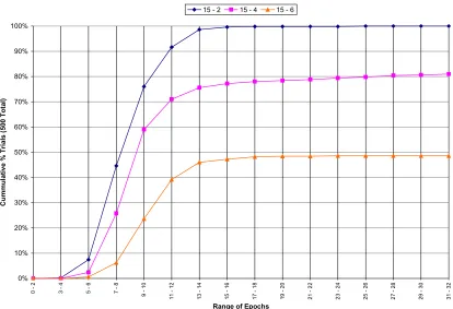
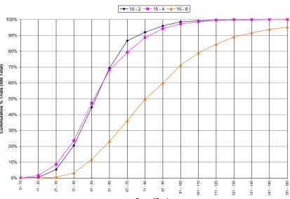
Another useful way to compare the data that generated Table 12 is to construct and plot empirical cumulative distribution functions from the data, as seen in Figures 11 through 13, below.

Figure 11: Empirical CDF of Percent Correct for Back-Prop Bit Counting

0% 10% 20% 30% 40% 50% 60% 70% 80% 90% 100% 10 0 9 9 99 9 8 98 9 7 9 7 - 96 96 9 5 95 9 4 9 4 - 93 93 9 2 92 9 1 91 9 0 90 8 9 8 9 - 88 8 8 - 87 87 8 6 86 8 5 8 5 - 84 84 8 3 83 8 2 8 2 - 81 8 1 - 80 80 7 9 79 7 8 78 7 7 77 7 6 7 6 - 75 75 7 4 74 7 3 73 7 2 7 2 - 71 71 7 0 70 6 9 69 6 8 6 8 - 67 6 7 - 66 66 6 5 65 6 4 64 6 3 6 3 - 62 62 6 1 61 6 0 6 0 - 59 5 9 - 58 58 5 7 57 5 6 56 5 5 5 5 - 54 54 5 3 53 5 2 52 5 1 5 1 - 50 50 4 9 49 4 8 48 4 7 47 4 6 4 6 - 45 45 4 4 44 4 3 43 4 2 4 2 - 41 41 4 0 40 3 9 39 3 8 3 8 - 37 37 3 6 36 3 5 35 3 4 3 4 - 33 3 3 - 32 32 3 1 31 3 0 30 2 9 2 9 - 28 28 2 7 27 2 6 26 2 5 2 5 - 24 24 2 3 23 2 2 22 2 1 2 1 - 20 20 1 9 19 1 8 18 1 7 1 7 - 16 1 6 - 15 15 1 4 14 1 3 1 3 - 12 1 2 - 11 11 1 0 10 9 9 - 8 8 7 7 - 6 6 - 5 5 - 4 4 3 3 - 2 2 - 1 1 - 0

Range of % Correct

C u m m u la ti ve % T ri al s (5 00 T o ta l)

Figure 12: Empirical CDF of Percent Correct for C-G Bit Counting

Figure 13: Empirical CDF of Percent Correct for Finite-Diff Bit Counting

0% 10% 20% 30% 40% 50% 60% 70% 80% 90% 100% 10 0 9 9 99 9 8 98 9 7 9 7 - 96 96 9 5 95 9 4 9 4 - 93 93 9 2 92 9 1 91 9 0 90 8 9 8 9 - 88 8 8 - 87 87 8 6 86 8 5 8 5 - 84 84 8 3 83 8 2 8 2 - 81 8 1 - 80 80 7 9 79 7 8 78 7 7 77 7 6 7 6 - 75 75 7 4 74 7 3 73 7 2 7 2 - 71 71 7 0 70 6 9 69 6 8 6 8 - 67 6 7 - 66 66 6 5 65 6 4 64 6 3 6 3 - 62 62 6 1 61 6 0 6 0 - 59 5 9 - 58 58 5 7 57 5 6 56 5 5 5 5 - 54 54 5 3 53 5 2 52 5 1 5 1 - 50 50 4 9 49 4 8 48 4 7 47 4 6 4 6 - 45 45 4 4 44 4 3 43 4 2 4 2 - 41 41 4 0 40 3 9 39 3 8 3 8 - 37 37 3 6 36 3 5 35 3 4 3 4 - 33 3 3 - 32 32 3 1 31 3 0 30 2 9 2 9 - 28 28 2 7 27 2 6 26 2 5 2 5 - 24 24 2 3 23 2 2 22 2 1 2 1 - 20 20 1 9 19 1 8 18 1 7 1 7 - 16 1 6 - 15 15 1 4 14 1 3 1 3 - 12 1 2 - 11 11 1 0 10 9 9 - 8 8 7 7 - 6 6 - 5 5 - 4 4 3 3 - 2 2 - 1 1 - 0

Range of % Correct

C u m m u la ti ve % T ri al s (5 00 T o ta l)

4 6 8 10

0% 10% 20% 30% 40% 50% 60% 70% 80% 90% 100% 10 0 - 99 99 9 8 98 9 7 9 7 - 96 96 9 5 95 9 4 94 9 3 9 3 - 92 9 2 - 91 91 9 0 90 8 9 8 9 - 88 8 8 - 87 87 8 6 86 8 5 85 8 4 8 4 - 83 83 8 2 82 8 1 81 8 0 80 7 9 7 9 - 7 8 7 8 - 77 77 7 6 76 7 5 75 7 4 7 4 - 73 73 7 2 72 7 1 71 7 0 7 0 - 69 6 9 - 68 68 6 7 67 6 6 66 6 5 6 5 - 64 64 6 3 63 6 2 62 6 1 6 1 - 60 6 0 - 59 59 5 8 58 5 7 5 7 - 56 5 6 - 55 55 5 4 54 5 3 53 5 2 5 2 - 51 51 5 0 50 4 9 49 4 8 48 4 7 47 4 6 4 6 - 45 45 4 4 44 4 3 43 4 2 4 2 - 41 41 4 0 40 3 9 39 3 8 3 8 - 37 3 7 - 36 36 3 5 35 3 4 34 3 3 3 3 - 32 32 3 1 31 3 0 30 2 9 2 9 - 28 2 8 - 27 27 2 6 26 2 5 2 5 - 2 4 2 4 - 2 3 2 3 - 22 22 2 1 21 2 0 2 0 - 19 19 1 8 18 1 7 17 1 6 16 1 5 15 1 4 1 4 - 13 13 1 2 12 1 1 11 1 0 1 0 - 9 9 - 8 8 - 7 7 - 6 6 5 5 4 4 - 3 3 - 2 2 - 1 1 0

Range of % Correct

C u m m u la ti ve % T ri al s (5 00 T o ta l)

From the preceding figures one can conclude that for hidden layer sizes of 6, 8, and 10 neurons the conjugate-gradient algorithm's statistical performance was superior to the other two algorithms. One curious feature of these figures, however, is that the back-prop algorithm appears to have outperformed the other two with a hidden layer size of 4.

2. How much work was required to complete the training?

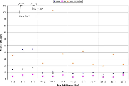
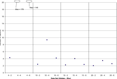
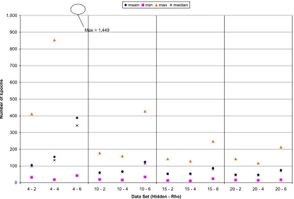
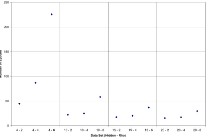
Again the amount of work required to train the network will be evaluated by comparing the distributions of the number of epochs necessary to train the network. The summary statistics of the distributions generated during the bit counting trials are shown below in Table 13.

Algorithm Hidden Layer Size Min.

Epochs Mean Epochs

Median Epochs

Max. Epochs

StDev Epochs

Back-Propagation 4 5,574 11,725 11,370 15,000 2,842

Back-Propagation 6 1,411 5,346 4,630 15,000 3,062

Back-Propagation 8 1,071 2,745 2,768 11,534 958

Back-Propagation 10 967 2,107 1,959 4,682 696

Conjugate-Gradient 4 215 6,837 3,227 15,000 6,241

Conjugate-Gradient 6 105 3,323 1,775 15,000 3,903

Conjugate-Gradient 8 74 1,166 684 15,000 1,520

Conjugate-Gradient 10 70 584 384 4,033 560

Finite-Difference 4 2,148 14,649 15,000 15,000 1,821

Finite-Difference 6 908 10,116 14,949 15,000 5,322

Finite-Difference 8 826 5,822 3,676 15,000 4,792

Finite-Difference 10 801 3,263 2,332 15,000 2,879

Table 13: Bit Counting Epochs Summary Statistics (All Data)

Figure 14: Empirical CDF of Epochs for Back-Prop Bit Counting

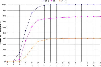
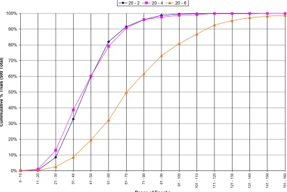
Figure 15: Empirical CDF of Epochs for C-G Bit Counting

0% 10% 20% 30% 40% 50% 60% 70% 80% 90% 100% 0 - 5 00 50 1 - 1 00 0 1 00 1 - 15 0 0 15 0 1 - 20 00 20 01 2 50 0 25 01 3 00 0 30 01 3 5 00 35 0 1 - 40 00 40 01 4 50 0 45 01 5 00 0 50 01 5 50 0 55 01 6 00 0 60 01 6 50 0 65 01 7 00 0 70 0 1 - 75 00 75 01 8 00 0 80 01 8 50 0 8 50 1 - 90 00 90 0 1 - 95 00 95 01 1 00 00 10 00 1 - 10 50 0 10 50 1 - 11 00 0 11 00 1 - 11 50 0 11 50 1 - 12 00 0 12 00 1 - 1 25 00 12 5 01 1 30 00 13 0 01 1 35 0 0 13 50 1 - 14 00 0 1 40 01 1 45 00 14 50 1 - 15 00 0 15 00 1 1 55 00

Range of Epochs

C u m m u la ti ve % T ri al s (5 00 T o ta l)

4 6 8 10

0% 10% 20% 30% 40% 50% 60% 70% 80% 90% 100% 0 - 50 0 50 1 - 10 00 10 01 1 50 0 1 50 1 - 20 00 2 00 1 - 25 00 25 0 1 - 30 00 30 01 3 50 0 35 01 4 00 0 40 01 4 50 0 45 0 1 - 50 00 50 0 1 - 55 00 55 01 6 00 0 60 01 6 50 0 65 01 7 00 0 70 0 1 - 75 00 75 01 8 00 0 80 01 8 50 0 85 01 9 00 0 90 0 1 - 95 0 0 95 01 1 00 00 10 00 1 - 10 50 0 10 50 1 - 11 00 0 1 10 01 1 15 00 11 5 01 1 20 00 12 00 1 1 25 00 12 50 1 - 13 00 0 1 30 01 1 35 00 13 5 01 1 40 00 14 0 01 1 45 00 14 50 1 1 50 00 15 00 1 - 15 50 0

Range of Epochs

C u m m u la ti ve % T ri al s (5 00 T o ta l)

Figure 16: Empirical CDF of Epochs for Finite-Diff Bit Counting

As with pattern recognition, so with bit counting – the conjugate-gradient algorithm required far fewer iterations for each hidden layer size than the other two algorithms by any statistical measure.

Therefore, the results of this study suggest that the conjugate-gradient algorithm was superior to the other two algorithms for bit counting as well. Figures 12 and 15 suggest that within the conjugate-gradient data set, the network with a hidden layer of 6 neurons gave the best overall accuracy performance with an acceptable trade-off in the distribution of epochs.

Conclusions and Future Work

All three algorithms were able to teach the pattern recognition task with near-perfect accuracy regardless of the hidden layer size chosen. The conjugate-gradient algorithm required much fewer training epochs to do so by any statistical measure. Therefore the data suggests that the conjugate-gradient algorithm was the best of the three algorithms for teaching the pattern recognition task. The bit counting problem proved much more difficult for all three training algorithms, but again, the statistical

0% 10% 20% 30% 40% 50% 60% 70% 80% 90% 100%

0

-

50

0

50

1

-

10

00

10

01

1

50

0

1

50

1

-

20

00

2

00

1

-

25

00

25

0

1

-

30

00

30

01

3

50

0

35

01

4

00

0

40

01

4

50

0

45

0

1

-

50

00

50

0

1

-

55

00

55

01

6

00

0

60

01

6

50

0

65

01

7

00

0

70

0

1

-

75

00

75

01

8

00

0

80

01

8

50

0

85

01

9

00

0

90

0

1

-

95

0

0

95

01

1

00

00

10

00

1

-

10

50

0

10

50

1

-

11

00

0

1

10

01

1

15

00

11

5

01

1

20

00

12

00

1

1

25

00

12

50

1

-

13

00

0

1

30

01

1

35

00

13

5

01

1

40

00

14

0

01

1

45

00

14

50

1

1

50

00

15

00

1

-

15

50

0

Range of Epochs

C

u

m

m

u

la

ti

ve

%

T

ri

al

s

(5

00

T

o

ta

l)

results of this study demonstrate the overall superiority of the conjugate-gradient relative to the other two.

The fact that a simple problem like bit counting should prove to be much harder for the network to learn than pattern recognition begs some explanation. One reason

could have to do with the concept of Hamming distances. The Hamming distance

between two vectors is defined as the number of components in which the two vectors

differ in value26._{. As a representative example, Table 14 below shows the Hamming}

distances between the vector (0, 0, 0) and each of the other vectors of 0 or 1 of length 3.

Vector 1 Vector 2 Hamming Distance

(0, 0, 0) (0, 0, 0) 0

(0, 0, 0) (0, 0, 1) 1

(0, 0, 0) (0, 1, 0) 1

(0, 0, 0) (0, 1, 1) 2

(0, 0, 0) (1, 0, 0) 1

(0, 0, 0) (1, 0, 1) 2

(0, 0, 0) (1, 1, 0) 2

(0, 0, 0) (1, 1, 1) 3

Table 14: Example Hamming Distances

The pattern recognition problem in this study has 10 unique input vectors and 10 corresponding unique output vectors, a one-to-one input-output functional relationship. This can be rephrased in terms of Hamming distances as follows: in pattern recognition, when the Hamming distance between two input vectors is greater than zero, the

Hamming distance between the corresponding output vectors will also be greater than zero. On the contrary, the 7-digit bit counting problem has 128 unique vectors but only 8 unique output vectors, a many-to-one functional relationship. Again, in terms of

Hamming distances: in bit counting, when the Hamming distance between two input vectors is greater than zero, the Hamming distance between the corresponding output vectors will be greater than or equal to zero. The conjecture that the results of this study suggest is that MLPs are more easily trained to perform tasks whose functional model is one-to-one than those whose model is one-to-many or many-to-one.

Some suggestions for future work are listed as follows:

thought behind the higher ρ values is that larger errors would be “trained out” more quickly by the corresponding higher order gradients that would result. However, this is only true when the absolute value of the error signal is greater than or equal to one. When this value is less than one, the larger ρ values would make the gradient much smaller, which could cause small but appreciable error signals to persist.

- Try a variable/adaptive finite-difference epsilon to try and improve the performance of the finite-difference algorithm.

References

1.) Rosenblatt, F., 1958. “The Perceptron: A probabalistic model for information storage and organization in the brain”, Psychological Review, vol. 65, pp. 386-408.

2.) Haykin, S. Neural Networks: A Comprehensive Foundation. 2nd _{Ed. New Jersey:}

Prentice-Hall; 1999. pp. 63-64. 3.) Ibid., pp.156-159.

4.) Ibid., pp.159-161. 5.) Ibid., pp. 168-169. 6.) Ibid., pp. 135-137. 7.) Ibid., p. 160. 8.) Ibid., p. 162. 9.) Ibid., pp. 179-181.

10.) LeCun, Y., 1993. Efficient Learning and Second-order Methods, A Tutorial at NIPS 93, Denver.

11.) Haykin, 1999. p. 184. 12.) Ibid., p. 184.

13.) Ibid., p. 63.

14.) Minsky, M.L., 1961. “Steps towards artificial intelligence”, Proceedings of the Institute of Radio Engineers, vol. 49, pp. 8-30.

15.) Rumelhart, D.E., G.E. Hinton, and R.J. Williams, 1986a. “Learning

representations of back-propagation”, in D.E. Rumelhart and J.L McCleland, eds., vol 1, Chapter 8, Cambridge, MA: MIT Press.

16.) Hebb, D.O. The Organization of Behavior: A Neuropsychological Theory. New York: Wiley; 1949. p. 62.

17.) Haykin, 1999. pp. 162-163. 18.) Ibid., pp. 164-166.

19.) Shewchuck, J.R. 1994. “An Introduction to the Conjugate Gradient Method

Without the Agonizing Pain” [Online]. Available from:

http://www-2.cs.cmu.edu/jrs/jrspapers.html#cg. pp.21-24.

20.) Haykin, 1999. pp. 237-238. 21.) Ibid., pp. 234-236.

24.) Polak, E., and G. Ribiere, 1969. “Note sur la convergence de methods de directions conjuguees”, Revue Francaise Information Recherche Operationnelle, vol. 16, pp. 35-43.

25.) Haykin, 1999. pp. 239-240.

26.) Paul E. Black, “Hamming distance”, in Dictionary of Algorithms and Data Structures [Online], Paul E. Black, ed., U.S. National Institute of Standards and Technology. May 31, 2006. Available from

Appendices

Appendix A: Pattern Recognition Calculator Digits