Using floating catchment area (FCA) metrics to predict health care utilization patterns

R E S E A R C H A R T I C L E

Open Access

Using floating catchment area (FCA)

metrics to predict health care utilization

patterns

Paul L. Delamater

, Ashton M. Shortridge

and Rachel C. Kilcoyne

Abstract

Background:Floating Catchment Area (FCA) metrics provide a comprehensive measure of potential spatial accessibility to health care services and are often used to identify geographic disparities in health care access. An unexplored aspect of FCA metrics is whether they can be useful in predicting where people actually seek care. This research addresses this question by examining the utility of FCA metrics for predicting patient utilization patterns, the flows of patients from their residences to facilities.

Methods:Using more than one million inpatient hospital visits in Michigan, we calculated expected utilization patterns from Zip Codes to hospitals using four FCA metrics and two traditional metrics (simple distance and a Huff model) and compared them to observed utilization patterns. Because all of the accessibility metrics rely on the specification of a distance decay function and its associated parameters, we conducted a sensitivity analysis to evaluate their effects on prediction accuracy.

Results:We found that the Three Step FCA (3SFCA) and Modified Two Step FCA (M2SFCA) were the most effective metrics for predicting utilization patterns, correctly predicting the destination hospital for nearly 74% of hospital visits in Michigan. These two metrics were also the least sensitive to changes to the distance decay functions and parameter settings. Conclusions:Overall, this research demonstrates that FCA metrics can provide reasonable predictions of patient utilization patterns and FCA utilization models could be considered as a substitute when utilization pattern data are unavailable.

Keywords:Spatial accessibility, Access to health care, Health care use, Utilization patterns, Hospitalizations, Floating catchment areas

Background

Much of the recent geographic research regarding access to health care has focused on examinations ofpotentialaccess to services, rather than onrealized access or utilization of health care services [1]. As defined by Aday and Anderson [2], potential access may be considered as a measure of the potential for entry into the health care system or a characterization of the level of opportunity provided by the health care delivery system. Conversely, realized access is a measure of actual utilization of a health care service, such that any barriers to the use of services have been overcome and access has been achieved. Penchansky and Thomas [3]

further examined the concept of potential access, providing five distinct dimensions of access, which Khan [4] later cat-egorized into spatial components (accessibility and avail-ability) and aspatial components (affordability, acceptability, and accommodation).

The fusion of accessibility (distance to services) and availability (volume of services) has been termedspatial

accessibility [5]. The Floating Catchment Area (FCA)

family of metrics simultaneously integrate the three essential components required to measure potential spatial accessibility: supply of services, potential demand for services, and distance separating supply and demand locations. Much of the recent FCA-related research has focused on methodological improvements to the metrics (e.g., [6–8]) or using the metrics to map and identify dis-parities in health care accessibility (e.g., [9–11]).

* Correspondence:[email protected]

1_{Department of Geography and the Carolina Population Center, University of} North Carolina at Chapel Hill, Chapel Hill, NC 27599, USA

Full list of author information is available at the end of the article

Less effort has been dedicated to understanding how potential spatial accessibility affects health care utilization. While there certainly are exceptions to this statement (e.g., [12–15]), the emphasis of potential spatial accessibility research has largely remained on “potential”. Ngui and Apparcio [16] note the complex nature of incorporating potential and realized informa-tion within a single study design, which may be one factor limiting research in this area. However, this deficit could simply be a result of differences in data availabi-lity; detailed health care utilization data is not always readily available to researchers due to privacy concerns, while health care facility locations and geographic popu-lation data are relatively easy to obtain.

People who live in the same region may utilize care at numerous facilities. Data representing the number of people residing in each region who use health care at mul-tiple facilities are referred to asutilization patternsor pa-tient flows. For a study area partitioned into n regions based on people’s residence and havingmfacilities located within it, utilization patterns are expressed as an n x m Origin-Destination (OD) matrix with the matrix entries containing the number of visits or volume of use for resi-dents of each region at each facility. Previous research on health care utilization patterns has generally been explana-tory in nature, focusing on identifying whether population and facility characteristics, as well as distance, affect where people receive care (e.g., [17–23]); less emphasis has been placed on developing models that provide accurate predic-tions of patient utilization patterns.

In this research, we evaluated the potential utility of using measures of spatial accessibility, namely FCA met-rics, to predict spatial patterns of health care utilization. Interestingly, the FCA metrics contain the requisite information to predict utilization patterns; however, they have yet to be evaluated in this capacity. We tested four FCA metrics, the Enhanced Two Step FCA (E2SFCA, [24]), the Modified 2SFCA (M2SFCA, [25]), the Three Step FCA (3SFCA, [26]), and a Huff-modified version of the 3SFCA (abbreviated H3SFCA for this work, [27]). Two traditional spatial accessibility approaches are im-plemented for comparative purposes: a simple distance-based approach and a Huff Model [28]. Each measure is highly dependent on the definition of a distance decay function and its parameter values. Thus, for each metric, we implemented four different distance decay functions, each having four parameter settings, to test for how characterization of distance decay affects the predictive accuracy of the metrics. Our approach produced a total of 96 outputs (6 metrics × 4 decay functions × 4 para-meter settings) that were compared against observed utilization patterns. We also examined one single metric, decay function, and parameter setting combination in detail to demonstrate the general nature of where the

predictions were most and least accurate to better understand the spatial distribution of predictive accuracy and factors that may have influenced it.

Methods

Input data and preprocessing

Our case study was conducted using inpatient hospitali-zations and hospitals in the state of Michigan (US). We evaluate all general acute care hospitalizations over an entire year in the state, as this is a nonspecialized, rela-tively common type of care. Michigan makes an ideal case study for several reasons, 1) as the largest state (by area) in the eastern United States, its nearly 10 million residents live in a wide range of representative commu-nities, from large urban cores and suburbs to rural and wilderness areas, 2) the geographic distribution of acute-care hospitals is spatially heterogeneous, leading to large variations in potential spatial accessibility, and 3) much of the state’s borders, along the Great Lakes and Canada, are effectively impassable for hospital service users, lessening the effects of study boundaries on models developed there.

Location and attribute data for hospitals in Michigan were acquired from the Michigan Department of Health and Human Services (MDHHS). The hospital attribute information was used to subset the data to only acute care hospitals offering emergency room ser-vices (n= 133) in an effort to remove hospitals providing only highly-specialized services that would be expected to draw patients under their own unique circumstances. The hospitalization utilization data was drawn from the 2014 Michigan Inpatient Database (MIDB), a hospital discharge database that contains, among other attributes, the resi-dential location of the patient (at the Zip Code level) and hospital visited for each inpatient hospitalization in the state (including Michigan residents visiting Michigan hos-pitals, Michigan residents who visited out of state hospi-tals, and out-of-state residents who visited Michigan hospitals). Zip Codes were used as the spatial population unit, as this is the most resolved location information in the MIDB. The patient discharges were subset to include only in-state residents visiting in-state hospitals, hereto-fore referred to as in-state visits (n = 1,063,721). Three hospitals did not report utilization data, thus were removed from the hospital data layer and analysis. One Zip Code had no in-state visits, thus was removed from the analysis.

A small number of manual adjustments were required to ensure the Zip Code layer matched the utilization data. US Census block polygons were downloaded from the Michigan Open Data Portal and converted to a point layer, with each point representing the geographic centroid of its corresponding Census block polygon. The total popula-tion in 2010 for each block was downloaded from the US Census (https://www2.census.gov) and joined to the spatial point layer. The block population points were then spatially joined to the Zip Code polygons and used to create the population-weighted centroid (PWC) each Zip Code, as well as to calculate the total population of each Zip Code.

Using the travel network, we constructed an OD matrix containing the estimated travel time from all Zip Code PWCs to all the acute care hospitals in Michigan. The travel time data were used to subset the hospitalization data to include only visits to hos-pitals that were less than or equal to 90 min from the patients’ residential addresses. This step was required to remove visits that most likely occurred while the patients were away from their residence or visits that required a type of health care service that was not available in their local region. The visits data were ag-gregated (summed) by Zip Code and hospital and stored in an OD matrix with the Zip Codes as ori-gins, the hospitals as destinations, and the number of visits (counts) as the entries. One Zip Code was re-moved from the analysis at this stage because its resi-dents had no visits to a hospital within 90 min of the Zip Code. The final observed utilization patterns OD matrix contained 1,034,492 inpatient hospital visits (97.3% of all in-state visits), occurring at 130 hospitals and originating from 907 Zip Codes. Of the 25,795 potential unique OD pairs meeting the 90-min travel time threshold, 13,242 had at least one patient visit.

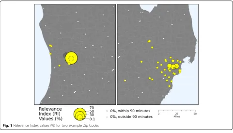
Using the visits OD matrix, we calculated the Rele-vance Index (RI) values, which normalizes for differ-ences in the total number of visits among Zip Codes [30]. The RI is calculated by dividing the number of visits by residents of the Zip Code i to each hospital j (Vi,j) by the total number of visits to all hospitals for that Zip Code (Vi):

RIi;j¼

Vi;j

Vi ð1Þ

This calculation produces a set of proportion values (scaled from 0 to 1) that sums to one for each Zip Code and represents normalized utilization patterns. The RIvalues for two example Zip Codes are mapped using a population perspective in Fig. 1 to illustrate this concept, showing one Zip Code with a large pro-portion of visits occurring at a single facility and

another Zip Code with visits more evenly dispersed across multiple facilities.

FCA metrics

The basic framework for all floating catchment area met-rics is based on a gravity model that integrates supply, de-mand, and distance simultaneously [31,32]. The history of these metrics and their formulation has been extensively published in previous work (e.g., [25]) thus is only briefly summarized here. While a number of FCA metrics could have been evaluated, the following summary is limited to those used in this analysis, which were chosen because they require a similar set of data to calculate: the location of potential demand (population counts), the location of facilities and their supply, and measures of the distance separating supply and demand locations, and have similar underlying assumptions in their formulation: a single travel mode, invariant distance thresholds or catchment sizes, and total population as potential demand.

The first step in the E2SFCA is to calculate the supply to demand ratio for each facility j (Dj) by dividing the supply (Sj) by the potential demand (Pj):

Dj¼

Sj P

i∈½di;j<dPiWi;j

ð2Þ

In this calculation, Pj is the distance-weighted sum of the population falling within a specified threshold distance (d) of facilityj,Piis the population at uniti, andWi,jis the weight assigned to distance di,j based on a specified dis-tance decay function. Common disdis-tance decay functions and their representation as weights can be found in Kwan [33] and Delamater [25], while the particular threshold distance parameter is often chosen based on the popula-tion distribupopula-tion within the study region (higher threshold distances include more remote populations). The second step in the E2SFCA is to calculate the distance-weighted sum of the supply to demand ratios falling within the threshold distance of each population uniti:

Ai¼ X

j∈½di;j<dDjWi;j ð3Þ

whereAiis the E2SFCA value.

The M2SFCA builds on the E2SFCA, but integrates an additional weight term in the formulation to account for the suboptimal distribution of supply locations. The first step is to calculate the supply to demand ratios for each facility and population unit combination (Di,j):

Di;j¼

SjWi;j P

i∈½di;j<dPiWi;j

ð4Þ

same as the E2SFCA, but the single facility supply to demand ratio is replaced by facility/unit value (Di,j):

Ai¼ X

j∈½di;j<dDi;jWi;j ð5Þ

The 3SFCA and H3SFCA both attempt to account for competition among facilities by adding an additional step to the E2SFCA formulation. The first step in each metric is to first calculate a selection weight (G), which defines the probability that a particular facility will be selected for use by a population. In the 3SFCA,Gi,jfor a population unitiand facilityjpairing is defined as:

Gi;j¼

Wi;j P

j∈½di;j<dWj

ð6Þ

The Gterm is simply based on distance (expressed as W) in the 3SFCA. The H3SFCA integrates a Huff Model to calculateGby incorporating both distance and supply in the formulation:

Gi;j¼

SjWi;j P

j∈½di;j<dSjWj

ð7Þ

The second and third steps of the 3SFCA and H3SFCA are the same as the two steps in the E2SFCA with the addition of theGterm:

Dj¼

Sj P

i∈½di;j<dPiWi;jGi;j

ð8Þ

and

Ai¼ X

j∈½di;j<dDjWi;jGi;j

ð9Þ

An interesting facet of all FCA-based metrics is that the final step includes, for each population uniti, a summa-tion of the supply to demand ratios for the set of facilities falling within the threshold distance, d. Hence, prior to this step, each FCA metric contains disaggregated infor-mation regarding the spatial accessibility that is provided by each facility for that population unit; however, given that the ultimate goal of the FCA metrics is to capture an overall measure of spatial accessibility for population units, this information is summed to calculate the finalAi value for each (i.e., Eqs.3, 5, and 9). Notably, the partial accessibility provided by each facility can be reconceptua-lized such that it describes the probability that people liv-ing in population unitiwill visit facilityj(pi,j), such that:

p_i;j¼Ai;j

Ai ð10Þ

(Ai) results in sets ofpi,j values that will always sum to one for each population unit and thus can be used to predict or estimate the proportion of each population unit that will use each facility. It is also important to note the connection between the RI values (Eq. 1) and the predicted probabilities from the partial spatial acces-sibility calculation in Eq. 10. The actual utilization pat-terns measured by RI values are directly comparable with the predicted utilization patterns based on spatial accessibility and represented aspvalues. This potentially highly valuable property of all FCA-based metrics has not been examined in previous research.

Potential spatial accessibility was calculated using four FCA metrics, the E2SFCA, M2SFCA, 3SFCA, and H3SFCA, using the number of hospital beds at each hospital as the measure of supply (S), the total popu-lation of each Zip Code as the potential demand (P), and the travel time from the PWC of each Zip Code to each hospital as the distance measure (d). The potential spatial accessibility values were converted to predicted probabilities of use per Eq.10. We also calculated a sim-ple distance-based measure of accessibility (DIST) using the selection weight formula from the 3SFCA (Eq. 6) and a simple Huff-based measure of accessibility (HUFF) using the selection weight formula from the H3SFCA (Eq. 7) for comparative purposes. The distance- and Huff-based accessibility values were also converted to predicted probabilities using Eq.10.

Distance decay functions

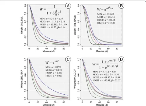
The FCA-, distance-, and Huff-based accessibility mea-sures all require a threshold distance and a distance decay function. The threshold distance is the distance at which a facility is no longer considered accessible, which was set at 90 min to mirror the constraints placed on the hospital utilization data. The choice of the particular distance decay function and its parameter value(s) can have a large effect on the resulting accessibility scores, as this governs the conversion of measured distances (d) to weight values (W). As a sensitivity analysis, we calcu-lated the metrics and corresponding predicted probabi-lities of utilization using four different decay functions, with each function having four unique parameter settings. The four functions were the Downward Log Logistic (DLL), Gaussian (GAUS), Exponential (EXP), and Logistic Cumulative Distance Function (LCDF), which have been used in similar work [7,25,33].

The parameter settings we used for each function cover a broad range of potential distance decay relation-ships. The processes used to generate the parameter set-tings is summarized here and detailed in the Additional file 1. The first set of parameter values for the decay functions was based on an estimate of distance decay if each person in the state uses their nearest

facility (MIN) and estimated by fitting the function to the data of the minimum distance to a facility. The next set of parameter values was based on the observed dis-tance decay observed in the hospitalization data (HOSP) and estimated by fitting the function to the observed hospital utilization data. The third set of parameter values (MOD) was calculated by taking the mean of the parameter values of MIN and HOSP, which represents “moderate” distance decay. The fourth set of parameter values (HIGH) was calculated by adding the difference between the second and third set of values back to the third set of values. The HIGH set of values represents a “high miss”when estimating the observed distance decay behavior. The distance decay weights for the four func-tions, along with the formulas and four parameter settings, are presented in Fig.2. As the figure shows, the four parameter settings cover a broad range of potential decay relationships for each function. While some of the function-parameter combinations fit the observed utilization data (e.g., DLL-HOSP), the combinations also include both functional forms and parameters settings that are very different from the observed distance decay. This range of both accurate and inaccurate combina-tions is important to evaluate, because the true distance decay relationship is generally not known when calculat-ing potential spatial accessibility since utilization data are not available.

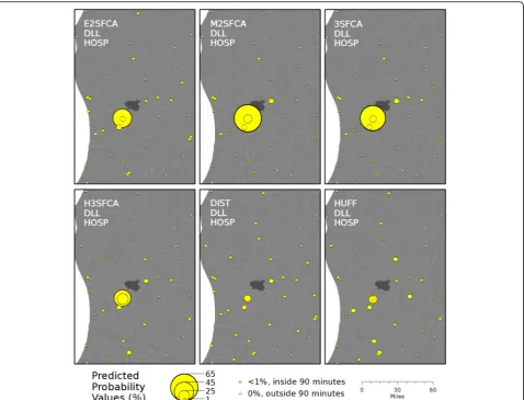
To illustrate the differences in the predicted probabi-lities of use among the six metrics, they are mapped for a single example Zip Code in Fig.3(using the DLL func-tion and HOSP parameter setting). Example figures show-ing the differences in predicted probabilities due to changes in the distance decay function and the decay func-tion’s parameter settings can be found in Additional file1.

Comparison with observed utilization patterns

Because the potential spatial accessibility metrics only produced probabilities of utilizing each facility (Eq. 10), we generated predicted visit counts from each Zip Code to each facility by multiplying the total number of hospital visits for each Zip Code by the predicted pro-bability values. As such, the total number of predicted hospital visits for each Zip Code was apportioned to fa-cilities based on the probabilities of utilization gathered from each spatial accessibility metric.

To assess the accuracy of each spatial accessibility metric, we first calculated the percent of patient visits that were correctly predicted. For each Zip Code, the observed number of visits to each facility was sub-tracted from the predicted number of visits to calcu-late the prediction error. This resulted in a prediction error matrix containing both under and over predic-tions (negative and positive values) that summed to 0 because of the bound nature of visits. For example, if a single hospital visit was mistakenly assigned to Hos-pital A instead of HosHos-pital B, this mistake would be recorded in the prediction error matrix as + 1 error

at Hospital A and−1 error at Hospital B. Hence, to calculate the percent correct based on counts, we first summed all of the positive prediction errors in the matrix, and then subtracted this sum from the total number of visits in the state. This calculation pro-duced the number of visits that were correctly pre-dicted, which was divided by the total number of visits to calculate the statewide percent of visits from each Zip Code to each Hospital that were correctly predicted. This calculation was performed for each spatial accessibility metric, decay function, parameter setting combination. An example of this calculation is provided in Additional file 1.

To calculate the percent correct based on the propor-tion of visits, we first used the above approach to calcu-late the percent correct for each Zip Code separately. Then, we calculated the mean percent correct over all Zip Codes. As such, this second measure of accuracy does not weigh by the differing number of visits origin-ating from each Zip Code and therefore represents each spatial accessibility metric, decay function, parameter Fig. 2Weight values and formulas for the distance decay functions. The four function forms area) Downward Log Logistic (DLL),b) Gaussian

(GAUS),c) Exponential (EXP), andd) Logistic Cumulative Distance Function (LCDF). The four parameter settings for each function are MIN (black),

setting combination’s ability to predict normalized utilization patterns (RI values). Additional file 1 also contains an example of this calculation.

We performed a detailed analysis for a single metric, decay function, and parameter combination to better understand the spatial distribution of the errors of prediction and their potential causes. Not-ably, we wanted to understand whether the number of facilities in the local region or the distribution of utilization among facilities (e.g., see Fig. 1) affected the ability of the metrics to predict patterns of utilization for each Zip Code. We tabulated the number of facilities within 90 min of each Zip Code. We calculated the Shannon Evenness Index (E, [34,

35]) using the observed RI values of hospitals within 90 min of each Zip Code as a measure of the even-ness of use across facilities. Potential E values range from 0 (all utilization at a single facility) to 1 (per-fectly even distribution of utilization across multiple facilities).

Results

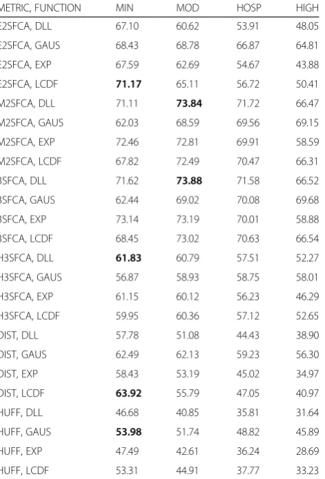
The percent of visits correctly predicted based on counts for each spatial accessibility metric, decay function, and parameter combination are found in Table 1. The most accurate metric-function-parameter combinations were

the 3SFCA-DLL-MOD (73.88% correct) and

M2SFCA-DLL-MOD (73.84%), which were followed closely by the E2SFCA-LCDF-MIN (71.71%). The most accurate combinations for the three other metrics were each under 65%. The accuracy of the nearest facility approach was 38.9%, which nearly all metric-function--parameter combinations largely outperformed. The sen-sitivity test of the metrics to the decay functions and parameter settings also provided interesting findings. Notably, the range of the percent correct for the 3SFCA, M2SFCA, and H3SFCA were each less than 16% (less sensitive), while the E2SFCA, DIST, and HUFF metrics each had a range greater than 25% (more sensitive).

parameter combination. Notably, the maximum values in Table 2 all are lower than the corresponding count-based results in Table 1, signaling that, in general, the accuracy of the spatial accessibility metrics was influ-enced by the raw count of visits. The M2SFCA, 3SFCA, and E2SFCA were again the most accurate in predicting utilization patterns. Interestingly though, the decay-par-ameter combinations with the most accurate results were not the same as the count-based results. The M2SFCA-DLL-HOSP (68.9% correct) and 3SFCA-EXP-HOSP (68.1%) were the most accurate in predicting nor-malized patterns of utilization, followed by the E2SFCA-EXP-MIN (66.14%). The H3SFCA, DIST, and HUFF metrics were lower in this measure of accuracy as well, having maximums of 57.78, 57.46, and 51.1% correct respectively. The nearest facility approach had an accuracy of 39.8% correct and, overall, the spatial accessibility rics outperformed this approach. The sensitivity of the met-rics to variations in the distance decay function and

parameter was quite different using the normalized utilization patterns. The least sensitive metric was the H3SFCA with a range of only 7.68%, although all combi-nations were quite low in accuracy comparatively. The range of the other metrics was between 14.69 and 18.14%, which was similar to the count-based results.

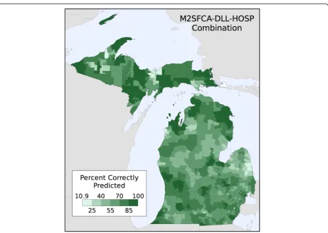
The percent of hospital visits correctly predicted by the M2SFCA-DLL-HOSP combination is mapped by Zip Code in Fig. 4. This combination was chosen because it was the best predictor of normalized utilization patterns and third highest predictor of the count-based utilization patterns. Using this metric, the minimum percent cor-rectly predicted for any Zip Code was 10.9%, while the maximum was 99.9% (after removing a Zip Code with only a single hospital within 90 min because it was 100% correctly predicted). The map shows that there was high heterogeneity throughout the state, as this metric was very accurate in some regions and quite inaccurate in others.

Table 1Percent of hospital visits (based on counts) correctly predicted

METRIC, FUNCTION MIN MOD HOSP HIGH

E2SFCA, DLL 67.10 60.62 53.91 48.05

E2SFCA, GAUS 68.43 68.78 66.87 64.81

E2SFCA, EXP 67.59 62.69 54.67 43.88

E2SFCA, LCDF 71.17 65.11 56.72 50.41

M2SFCA, DLL 71.11 73.84 71.72 66.47

M2SFCA, GAUS 62.03 68.59 69.56 69.15

M2SFCA, EXP 72.46 72.81 69.91 58.59

M2SFCA, LCDF 67.82 72.49 70.47 66.31

3SFCA, DLL 71.62 73.88 71.58 66.52

3SFCA, GAUS 62.44 69.02 70.08 69.68

3SFCA, EXP 73.14 73.19 70.01 58.88

3SFCA, LCDF 68.45 73.02 70.63 66.54

H3SFCA, DLL 61.83 60.79 57.51 52.27

H3SFCA, GAUS 56.87 58.93 58.75 58.01

H3SFCA, EXP 61.15 60.12 56.23 46.29

H3SFCA, LCDF 59.95 60.36 57.12 52.65

DIST, DLL 57.78 51.08 44.43 38.90

DIST, GAUS 62.49 62.13 59.23 56.30

DIST, EXP 58.43 53.19 45.02 34.97

DIST, LCDF 63.92 55.79 47.05 40.97

HUFF, DLL 46.68 40.85 35.81 31.64

HUFF, GAUS 53.98 51.74 48.82 45.89

HUFF, EXP 47.49 42.61 36.24 28.69

HUFF, LCDF 53.31 44.91 37.77 33.23

Legend: The spatial accessibility metric and decay function are in the rows and the decay functions’parameter settings are in the columns. The highest accuracy combination for each metric is in bold text

Table 2Percent of hospital visits (based on proportions) correctly predicted

METRIC, FUNCTION MIN MOD HOSP HIGH

E2SFCA, DLL 64.17 61.55 57.67 53.60

E2SFCA, GAUS 57.15 61.15 63.18 64.22

E2SFCA, EXP 66.14 64.53 59.85 51.45

E2SFCA, LCDF 63.62 65.57 61.43 56.95

M2SFCA, DLL 64.75 68.08 68.90 66.88

M2SFCA, GAUS 52.33 57.52 60.27 62.16

M2SFCA, EXP 64.31 67.03 68.53 63.28

M2SFCA, LCDF 57.82 65.45 68.23 67.66

3SFCA, DLL 64.60 67.05 67.65 65.99

3SFCA, GAUS 52.66 58.12 60.96 62.75

3SFCA, EXP 64.82 66.96 68.10 63.10

3SFCA, LCDF 58.57 65.70 67.93 67.35

H3SFCA, DLL 57.18 57.23 55.92 53.09

H3SFCA, GAUS 50.10 53.14 54.59 55.54

H3SFCA, EXP 57.28 57.78 56.56 50.55

H3SFCA, LCDF 54.04 57.43 57.11 54.95

DIST, DLL 53.65 49.99 45.76 41.75

DIST, GAUS 53.61 56.03 56.21 55.63

DIST, EXP 56.28 53.42 47.82 39.50

DIST, LCDF 57.46 55.18 49.57 44.90

HUFF, DLL 44.99 41.44 37.92 34.66

HUFF, GAUS 49.23 49.88 49.28 48.19

HUFF, EXP 48.15 44.88 39.78 32.97

HUFF, LCDF 51.10 46.80 41.34 37.34

Figure 5a shows the number of hospitals within 90 min of each Zip Code and Fig. 5b shows the Shannon’s

Evenness Index values based on observed utilization pat-terns. The concentration of hospitals in the southeast portion of Michigan is apparent, which is where much of the state’s population resides. The places with the highest number of hospitals within 90 min are located in the region between metro Detroit, Lansing, Ann Arbor, and Saginaw. The most obvious pattern in the evenness map are the low values (indicating utilization largely oc-curs at a single or very few facilities) found in and around population centers in the southern part of the state, which have a small number of large hospitals and the low values in and around the larger, regional hospi-tals found throughout the northern part of the state. High values of evenness are found in many of the regions located “in between” population centers, indi-cating utilization is distributed among multiple hospitals. The percent of hospital visits correctly predicted using the M2SFCA-DLL-HOSP combination is plotted against the number of hospitals within 90 min of each Zip Code in Fig. 6a and against the Shannon Evenness Index values in Fig. 6b. The plots do not provide strong

evidence of a systematic effect on the M2SFCA’s ability to predict patterns of utilization based on the potential number of hospitals or the evenness of utilization across hospitals. Interestingly, the greatest range in predictive accuracy is found at the lower end of the distribution of both variables. This is a somewhat counterintuitive find-ing in that fewer hospitals nearby and more concen-trated utilization across hospitals could be considered a less complex scenario (than evenly distributed hospital visits across numerous hospitals) to attempt to predict.

Discussion

Fig. 6Percent of hospital visits correctly predicted for each Zip Code. Predictions were made using the M2SFCA-DLL-HOSP combination plotted

against (a) the number of hospitals within 90 min of each Zip Code and (b) the Shannon’s Evenness Index values. The number of points in each

hexagon ranges from 1 (white) to 18 (black)

more than 25,000 potential origin destination pairs. All of the FCA metrics provided substantial gains in predict-ive accuracy over the simple nearest facility approach. Specifically, the E2SFCA, 3SFCA, and M2SFCA pro-duced the most accurate predictions using count-based and normalized utilization patterns.

Our results suggest that FCA metrics have potential for use in estimating where people go to receive health care in the absence of detailed utilization data and as an alternative to the assumption that people use the nearest facility. This information can be useful in a number of circumstances. First, it can be directly applied for plan-ning purposes; specifically, if some regions are expected to need a higher volume of services in the future, esti-mated utilization patterns could be used to predict which facilities may require more resources to meet that future demand.

Another potential use is to use utilization pattern esti-mates in understanding health outcomes as they relate to where people are receiving health services. A com-mon issue faced in health services research is how to ac-count for variations in facility quality or other aspects of service provision when examining population-level utilization and health outcomes. For this purpose, the estimated utilization patterns can be integrated within an analysis to assign facility-level information to popula-tions based on the estimated proportion of people using each facility.

Another circumstance in which our findings may be useful is when a researcher has utilization data at the facility-level, but does not have information about the residential location of the people who visited each facil-ity. Whereas our work focused on predicting the destin-ation aspect of utilization patterns, the approach could be reconfigured to predict patient origins. While this would require further analysis and evaluation of this modified approach, it has the potential to provide valuable estimates of where patients originated in the absence of this information. Specifically, it might be used by facilities to better understand the underlying popula-tion from which their patient base is drawn.

The results of the sensitivity analysis showed that the accuracy of the predictions for all metrics was af-fected by the choice of the particular distance decay function and its parameters. A known limitation of spatial accessibility metrics that use distance decay in their formulation is that the output will vary given changes to the decay function or parameter settings [24, 36, 37]. Further, there is often little guidance from prior research to justify using one function or parameter setting over another. It is difficult to disen-tangle the reasons why some of the metrics were more affected by the variations in distance decay than others because the decay function, its parameters, and

the metric’s formulation all are working simultan-eously to characterize spatial accessibility. Because most researchers will not have access to observed data that can be used to evaluate the accuracy of utilization predictions made using spatial accessibility metrics, we suggest caution in using FCA metrics for predicting utilization patterns without considering this limitation. However, an important takeaway from the sensitivity analysis is that many of the metrics’ predic-tions were more accurate when the distance decay function parameter(s) resulted in a stronger decay ef-fect. The MIN parameter set generally produced more accurate results than the HIGH parameter set (high miss) in both the count-based and normalized predic-tions for a number of metrics. This finding is import-ant because the MIN parameter set does not require any utilization data to be estimated; it only requires population counts (and locations), facility locations, and the distance separating people and facilities, which are the same inputs needed to calculate an FCA metric and can be readily obtained for many study areas. Another noteworthy result is that the HOSP parameter set, which was derived directly from the utilization data, did not always provide the most accurate results. This suggests that knowing the glo-bally averaged distance decay parameter set may not capture local variations in this relationship.

identifying regions where residents are traveling further than expected to access services and exami-ning whether this may be due to non-spatial barriers to accessing care, such as whether the nearby facilities offers the services required to meet the needs of the population.

Limitations

While this research did shed light on the overall po-tential of using FCA metrics to predict utilization pat-terns, it does have limitations. First, the case study only considered acute care hospitalizations in a single state in the US. The predictive power of FCA metrics, along with other empirical findings of this study, are surely rooted within the context of Michigan’s health care system and the socioeconomic, cultural, and geo-graphic context of the communities this system serves. Whether FCA metrics can predict utilization patterns for other health care services or in other US states or in other countries with highly different health care systems remains unknown but does present an avenue for further exploration.

A second limitation of this work was the omission of other factors known to influence where and how far patients travel to receive hospital care in the US, inclu-ding their ability to travel (mobility), their health insur-ance status, different travel modes available (e.g., public transit and personal vehicles), the services provided at each hospital, the perceived or measured quality of the hospitals, doctor admitting privileges, and others. These omissions were part of the research design for this work, as our aim was to evaluate the utility of a relatively naïve, oft-encountered, and easy to implement model (FCA metrics) to predict use. As such, understanding how these other factors influence patient utilization pat-terns and whether they interact with potential spatial accessibility is an important opportunity for future research. Specifically, determining whether these factors played a role in the geographic variation in the predic-tive ability of the FCA metrics may potentially uncover how other aspects of potential access to care affect where people utilize facilities.

A third limitation of the analysis was the use of the number of bed licenses as a proxy for supply in the spatial accessibility metrics. While this measure is often used, it does not always capture a facility’s ac-tual supply or ability to provide care (e.g., if beds are not in use due to understaffing). In our study, we attempted to use as little auxiliary information as possible to mimic the conditions researchers would generally face when attempting to estimate utilization patterns from publicly-available facility data. Another data-related limitation is that three hospitals were

excluded from the analysis, as was one Zip Code, due to lack of data; however, the missing data from these facilities and Zip Code represent a miniscule fraction of the statewide hospitalization and we do not believe this had any effect on our results.

Another limitation is that our analysis demonstrated that the predictive accuracy of the FCA metrics was sen-sitive to the particular metric, distance decay function, and the decay function parameters. Thus, we are not able to provide a definitive answer to which combination should be used in other circumstances, especially when researchers do not have the observed data to evaluate the accuracy of the predictions. While this does restrict the overall usefulness of this approach, we are encour-aged that all four FCA metrics were much more accur-ate than assuming people visited their nearest facility, an approach that is oft-employed in these types of scenar-ios. Furthermore, the MIN distance decay parameter set performed quite well across metrics and decay functions. This is important because this parameter set is based on the distance from populations to facilities and does not require any additional data beyond what is necessary to calculate the FCA metrics. Thus, this parameter set does not require utilization data and can be calculated in any scenario when the location of people and facilities are known.

Conclusions

Additional file

Additional file 1:Distance decay parameter generation methods and examples. (DOCX 410 kb)

Abbreviations

2SFCA:Two step floating catchment area; 3SFCA: Three step floating catchment area; DIST: Simple distance-based measure of accessibility; DLL: Downward log logistic distance decay function; E2SFCA: Enhanced two step floating catchment area; EXP: Exponential distance decay function; FCA: Floating catchment area; GAUS: Gaussian distance decay function; H3SFCA: Huff-modified three step floating catchment area; HIGH: Parameter

values for the decay functions representing a“high miss”when estimating

the observed distance decay behavior; HOSP: Parameter values for the decay functions based on the empirical distance decay observed in the hospital utilization data; HUFF: Huff-based model of accessibility; LCDF: Logistic cumulative distance decay function; M2SFCA: Modified two step floating catchment area; MDHHS: Michigan Department of Health and Human Services; MIDB: Michigan inpatient database; MIN: Parameter values for the decay functions based on an estimate of distance decay if each person in the state used the nearest facility; MOD: Parameter values for the decay

functions representing a_“moderate_”distance decay; OD: Origin-destination;

PWC: Population weighted centroid; RI: Relevance index

Acknowledgements

Not applicable.

Funding

We received financial support for this research from the Michigan Department of Health and Human Services (MDHHS), Certificate of Need Section. The funding source provided the MIDB data, but had no role in the research design, analysis, dissemination of the results, or decision to publish the manuscript.

Availability of data and materials

The publicly-available data sources have been provided in the main text. The hospitalization data that support the findings of this study are available from the Michigan Hospital Association (MHA), but restrictions apply to the avail-ability of these data, which were used under license for the current study, and so are not publicly available. Per the data use agreement among MHA, MDHHS, and the authors, the authors cannot redistribute the hospitalization data. Location and attribute data for hospitals in Michigan can be acquired from the corresponding author on reasonable request.

Authors’contributions

PD conceived the study and led the analysis. AS contributed to the research design. RC contributed to the data analysis. All authors contributed to the interpretation of the results from the analysis. PD drafted the manuscript. All authors revised the manuscript for important intellectual content. All authors read and approved the final manuscript.

Ethics approval and consent to participate

The Michigan Hospital Inpatient Database (MIDB) consists of routinely

collected information on patients’hospital discharges for billing purposes.

The patients provided written consent for their information to be stored in the hospital database. All identifiable patient information was removed from the MIDB prior for use in this research. The participants therefore, did not provide their written or verbal informed consent to participate in this study. Written consent was not obtained because identifiable information on patients was not available in the MIBD data used in this research. The Michigan State University Internal Review Board Ethics Committee approved this consent procedure and determined the use of the de-identifiable MIDB

data exempt for use in this research (IRB #07–362–April 23, 2012).

Consent for publication

Not applicable.

Competing interests

The authors declare that they have no competing interests.

Publisher’s Note

Springer Nature remains neutral with regard to jurisdictional claims in published maps and institutional affiliations.

Author details

1_{Department of Geography and the Carolina Population Center, University of} North Carolina at Chapel Hill, Chapel Hill, NC 27599, USA.2_{Department of} Geography, Environment, and Spatial Sciences, Michigan State University, East Lansing, MI 48824, USA.3_{Department of Geography and Geoinformation} Science, George Mason University, Fairfax, VA 22030, USA.

Received: 29 August 2018 Accepted: 21 February 2019

References

1. Higgs G. The role of GIS for health utilization studies: literature review.

Health Services Outcomes Res Methodology. 2009;9:84–99.

2. Aday LA, Andersen RA. Framework for the study of access to medical care.

Health Serv Res. 1974;9:208–20.

3. Penchansky R, Thomas JW. The concept of access: definition and

relationship to consumer satisfaction. Med Care. 1981;19:127_–40.

4. Khan AA. An integrated approach to measuring potential spatial access to

health care services. Socio Econ Plan Sci. 1992;26:275–87.

5. Guagliardo MF, Ronzio CR, Cheung I, Chacko E, Joseph JG. Physician

accessibility: an urban case study of pediatric providers. Health Place. 2004;

10:273_–83.

6. Fransen K, Neutens T, De Maeyer P, Deruyter G. A commuter-based

two-step floating catchment area method for measuring spatial accessibility of

daycare centers. Health Place. 2015;32:65–73.

7. Bauer J, Groneberg DA. Measuring spatial accessibility of health care

providers_–introduction of a variable distance decay function within the

floating catchment area (FCA) method. PLoS One. 2016;11:e0159148.

8. Langford M, Higgs G, Fry R. Multi-modal two-step floating catchment area

analysis of primary health care accessibility. Health Place. 2016;38:70–81.

9. Shah TI, Bell S, Wilson K. Spatial accessibility to health care services:

identifying under-serviced Neighbourhoods in Canadian urban areas. PLoS One. 2016;11:e0168208.

10. Vadrevu L, Kanjilal B. Measuring spatial equity and access to maternal

health services using enhanced two step floating catchment area

method (E2SFCA)–a case study of the Indian Sundarbans. Int J Equity

Health. 2016;15:87.

11. Nasseh K, Eisenberg Y, Vujicic M. Geographic access to dental care varies in

Missouri and Wisconsin. J Public Health Dent. 2017.

12. Lian M, Struthers J, Schootman M. Comparing GIS-based measures in access

to mammography and their validity in predicting neighborhood risk of late-stage breast Cancer. PLoS One. 2012;7:e43000.

13. Delamater PL, Messina JP, Grady SC, WinklerPrins V, Shortridge AM. Do more

hospital beds Lead to higher hospitalization rates? A spatial examination of

Roemer’s law. PLoS One. 2013;8:e54900.

14. Fishman J, McLafferty S, Galanter W. Does spatial access to primary care

affect emergency department utilization for nonemergent conditions? Health Serv Res 2016;n/a-n/a.

15. Alford-Teaster J, Lange JM, Hubbard RA, Lee CI, Haas JS, Shi X, et al. Is the

closest facility the one actually used? An assessment of travel time estimation based on mammography facilities. Int J Health Geogr. 2016;15:8.

16. Ngui A, Apparicio P. Optimizing the two-step floating catchment area

method for measuring spatial accessibility to medical clinics in Montreal.

BMC Health Serv Res. 2011;11(1):_–12.

17. Folland ST. Predicting hospital market shares. Inquiry. 1983;20:34–44.

18. Mayer JD. The distance behavior of hospital patients: a disaggregated

analysis. Soc Sci Med. 1983;17:819_–27.

19. McGuirk MA, Porell FW. Spatial patterns of hospital utilization: the impact of

distance and time. Inquiry. 1984;21:84–95.

20. Cohen MA, Lee HL. The determinants of spatial distribution of hospital

utilization in a region. Med Care. 1985;23:27–38.

21. McLafferty S. Predicting the effect of hospital closure on hospital utilization

patterns. Soc Sci Med. 1988;27:255–62.

22. Adams EK, Porell FW, Robbins JD. Estimating the utilization impacts of

hospital closures through hospital choice models: a comparison of

23. Lowe JM, Sen A. Gravity model applications in health planning: analysis of

an Urban Hospital market. J Reg Sci. 1996;36:437_–61.

24. Luo W, Qi Y. An enhanced two-step floating catchment area (E2SFCA)

method for measuring spatial accessibility to primary care physicians. Health

Place. 2009;15:1100–7.

25. Delamater PL. Spatial accessibility in suboptimally configured health care

systems: a modified two-step floating catchment area (M2SFCA) metric.

Health Place. 2013;24:30–43.

26. Wan N, Zou B, Sternberg T. A three-step floating catchment area

method for analyzing spatial access to health services. Int J Geogr Inf

Sci. 2012;26:1073–89.

27. Luo J. Integrating the Huff model and floating catchment area methods to

analyze spatial access to healthcare services. Trans GIS. 2014;18:436–48.

28. Huff DL. Defining and estimating a trading area. J Mark. 1964;28:34_–8.

29. Delamater PL, Messina JP, Shortridge AM, Grady SC. Measuring geographic

access to health care: raster and network-based methods. Int J Health

Geogr. 2012;11(1):–18.

30. Griffith JR. Quantitative techniques for hospital planning and control.

Lexington, MA: Lexington Books; 1972.

31. Radke J, Mu L. Spatial decompositions, modeling and mapping service

regions to predict access to social programs. Ann GIS. 2000;6:105–12.

32. Luo W, Wang F. Measures of spatial accessibility to health care in a GIS

environment: synthesis and a case study in the Chicago region.

Environment and Planning B: Planning and Design. 2003;30:865–84.

33. Kwan M-P. Space-time and integral measures of individual accessibility:

a comparative analysis using a point-based framework. Geogr Anal.

1998;30:191–216.

34. Pielou EC. Ecological diversity: Wiley; 1975.

35. Smith B, Wilson JB. A Consumer’s guide to evenness indices. Oikos.

1996;76:70_–82.

36. Schuurman N, Berube M, Crooks VA. Measuring potential spatial access to

primary health care physicians using a modified gravity model. Can Geogr.

2010;54:29–45.

37. Wan N, Zhan FB, Zou B. Chow E. A relative spatial access assessment

approach for analyzing potential spatial access to colorectal cancer services