Introduction to Linear, Time-Invariant, Dynamic Systems for Students of Engineering

Introduction to

Linear, Time-Invariant, Dynamic Systems

for

Students of Engineering

INTRODUCTION TO

LINEAR, TIME-INVARIANT, DYNAMIC SYSTEMS

FOR STUDENTS OF ENGINEERING

William L. Hallauer, Jr.

Permission of the author is granted for reproduction in any form of this book or any part of this book, provided that there is appropriate attribution, for example, by a citation in the References section of a technical article, and provided that the reproduction is not made for the purpose of charging a fee to users (e.g., students in a class) beyond the cost of reproduction.

However, plagiarism from this book is prohibited, and any use of the material in this book to produce profit or income beyond the cost of reproduction is prohibited.

© 2016 by William L. Hallauer, Jr.

Introduction to Linear, Time-Invariant, Dynamic Systems for Students of Engineering is licensed under a Creative Commons Attribution-NonCommercial 4.0 International License. For details of use requirements, please see https://creativecommons.org/licenses/by-nc/4.0/.

FOR STUDENTS OF ENGINEERING

William L. Hallauer, Jr.

AUTHOR’S PREFACE

I taught many times the college undergraduate, junior-level, one-semester course entitled “AOE 3034, Vehicle Vibration and Control” in the Department of Aerospace and Ocean Engineering (AOE) at Virginia Polytechnic Institute and State University (VPI & SU). I was dissatisfied using commercially available textbooks for AOE 3034, so I began writing my own course notes, and those notes grew into this book. Although this project began with preparation of informal handout notes, the completed book is a formal college engineering textbook, complete with homework problems at the end of each chapter, a detailed Table of Contents, a list of References, and a detailed Index. I hope that this book will be understandable and enlightening for students of engineering system dynam-ics, a valuable teaching resource for course instructors, and a useful reference for self-study and review.

The content of this book is based primarily on topics that the faculty of AOE and VPI & SU elected to include in AOE 3034 during the 1990s and early 2000s. The con-cise course description is: “Free and forced motions of first-order systems. Free and forced motions of second-order systems, both undamped and damped. Frequency and time responses. Introduction to control, transfer functions, block diagrams, and closed-loop system characteristics. Higher-order systems.” A more detailed course description

is provided by the following list of primary learning objectives, which were developed to

satisfy requirements of the agency that accredits engineering college degrees in the United States:

At the completion of AOE 3034, the student should be able to:

1. Solve first-, second-, and higher-order, linear, time-invariant (LTI) or-dinary differential equations (ODEs) with forcing, using both time-domain and Laplace-transform methods.

2. Solve for the frequency response of an LTI system to periodic sinusoi-dal excitation and plot this response in standard form (log magnitude and phase versus frequency).

4. Derive and analyze mathematical models (ODEs) for low-order me-chanical systems, both translational and rotational systems, that are com-posed of inertial elements, spring elements, and damping devices.

5. Derive and analyze mathematical models (ODEs) for low-order electri-cal systems (circuits) composed of resistors, capacitors, inductors, and op-erational amplifiers.

6. Derive (from ODEs) and manipulate Laplace transfer functions and block diagrams representing output-to-input relationships of discrete ele-ments and of systems.

7. Define and evaluate “stability” for an LTI system.

8. Explain “proportional”, “integral”, and “derivative” types of feedback control for single-input, single-output (SISO), LTI systems.

9. Sketch the locus of characteristic values, as a control parameter varies, for a feedback-controlled SISO, LTI system.

10. Use MATLAB1 as a tool to study the time and frequency responses of

LTI systems.

Rather that summarizing the contents of this book chapter by chapter, I invite the reader of this preface to peruse the detailed Table of Contents. However, the book’s gen-eral organization is the following: Chapters 1-10 deal primarily with the ODEs and be-haviors of first-order and second-order dynamic systems; Chapters 11 and 12 touch on

the ODEs and behaviors of mechanical systems having two degrees of freedom, i.e.,

fourth-order systems; Chapters 13 and 14 introduce classical feedback control, motivat-ing the concept with what I believe is a unique approach based on the standard ODE of a second-order dynamic system; Chapter 15 presents the basic features of proportional, in-tegral, and derivative types of classical control; and Chapters 16 and 17 discuss methods for analyzing the stability of classical control systems. The principal parts of Chapters 1-16 are focused on the ten primary learning objectives listed above. I added Chapter 17 on frequency-response stability analysis because I feel that an introduction to classical con-trol theory and design is incomplete without that subject, even though it was not included in AOE 3034.

The general minimum prerequisite for studying this book is the intellectual matur-ity of a junior-level (third-year) college student in an accredited four-year engineering curriculum. More specifically, a reader of this book should already have passed standard first courses in engineering dynamics and ODEs. It will be helpful if, but probably is not

1

mandatory that, the reader has studied basic electrical circuits, perhaps in an introductory college physics course. It is necessary that the reader has studied basic computer pro-gramming. MATLAB computer programs and commands appear throughout this book, so the reader should be able to understand MATLAB commands. However, MATLAB commands are generally clearly expressed in standard English and standard arithmetic notation, so a person who has done any computer programming, even if that was not with MATLAB, probably can follow the computer commands and command sequences in this book. Familiarity with matrix notation and matrix arithmetic operations also will be helpful, especially for Chapters 11 and 12. My students who took at the same time AOE 3034 and a mathematics course on operational methods (primarily Laplace transforms) often found that the combination of those courses was unusually complementary and beneficial to their comprehension of the material.

A mathematical second-order system is represented in this book primarily by a

single second-order ODE, not in the state-space form by a pair of coupled first-order

ODEs. Similarly, a two-degrees-of-freedom (fourth-order) system is represented in Chapters 11 and 12 by a pair of coupled second-order ODEs, not in the state-space form by four coupled first-order ODEs. A reader who can understand the mathematics and dynamics of relatively simple systems expressed here in classical second-order form probably will have little trouble making the transition in more advanced literature to the general state-space representation of higher order systems.

This book deals mostly with specific idealized models of basic physical systems, such as mass-damper-spring mechanisms and single-loop electrical circuits. The empha-ses are on fundamental ODEs and fundamental system response characteristics. I have

chosen, therefore, not to burden the reader with bond graph modeling, the general and

powerful, but complicated, modern tool for analysis of dynamic systems. However, the material in this book is an appropriate preparation for the bond graph approach presented

in, for example, System Dynamics: Modeling, Simulation, and Control of Mechatronic

Systems, 5th edition, by Dean C. Karnopp, Donald L. Margolis, and Ronald C. Rosenberg, published by John Wiley & Sons, 2012.

I intended originally that Chapters 1-16 of the course notes (before they grew into a book) could be covered in a normally-paced course of three fifty-minute lessons per week in a standard college semester of fourteen weeks duration. Even so, instructors of AOE 3034, including myself, had difficulty squeezing all of that content into forty-two lessons. Furthermore, in the process of converting the course notes into a complete text-book, I added material that is relevant and interesting (to me, at least) in many complete

“new” sections to the ends of Chapters 12, 7, 8, 10, 14, and 16. And, as mentioned

above, I also added a complete “new” Chapter 17. Consequently, I doubt that even the

2

most demanding course instructor can, while still treating the students fairly, cover this entire book in a three-credit, one-semester course. Therefore, instructors who wish to use this as a one-semester course textbook should decide in advance which parts of the book are essential to the course and which parts they cannot cover in the time allotted for the course. If, for example, it is essential to cover all of Chapters 13-17 on classical control, an instructor might elect to skip some or all of the “new” sections in Chapters 1, 7, 8, and 10, and to skip Chapters 11 and 12 on systems with two degrees of freedom, but to cover most everything else in the book. Sections 6-4, 6-5, and 8-11 deal primarily with compu-tational methods for calculating approximate time-response solutions of first- and second-order ODEs; the contents of these sections are nicely compatible with the chapters in which they reside; but they are not essential to the reader’s understanding of system dy-namics, so they can be omitted from course coverage without great loss. On the other hand, I discourage the omission of Chapter 5 on basic electrical systems, not only be-cause I believe the material is important to most engineers, but also bebe-cause such systems provide many examples and homework problems later in the book.

The homework problems at the ends of chapters are very important to the learning objectives of this book. I wrote each problem statement while at the same time preparing the solution, in order to help make the statements as clear, correct, and unambiguous as possible. In many cases, I stated a result, such as a Laplace transform, in a chapter’s text but left as a homework problem the proof or other development of that result. When teaching a lesson from the course notes that grew into this book, I would often not lecture on the material of the reading that I had assigned for the lesson. Instead, I would assume that the students had, in fact, completed and understood the assigned reading, summarize the main results of that reading and ask if there were questions about it, then, after sponding to any questions, spend most remaining lesson time discussing some of the re-lated homework problems.

A major focus of this book is computer calculation of system characteristics and responses and display of the results graphically, with use of MATLAB commands and programs. However, the book employs, for the most part, basic MATLAB commands and operations (aside from array operations), such as those on hand calculators; there is very little use of advanced MATLAB operations and functions, because these can pro-duce results without the user having to understand the processes of production. For this introductory material, I think it is important that the computer and software function as a “super calculator”, which relieves the user of the drudgery of calculations, especially complex and/or repetitive calculations, but still requires the user to understand the pro-cess well enough to be able to design and program the calculations and graphical dis-plays.

Since 1967 with the publication of Dynamics of Physical Systems by Robert H.

11 and 12, attitude control of spacecraft and aircraft in Chapters 14-16, and an analysis of aeroelastic flutter in the final homework problem of Chapter 16.

I favor illustrating and validating theory, whenever possible, with measured data. I also favor using measured data to identify system dynamic characteristics based on

mathematical models (e.g., time constants and natural frequencies), and system basic

properties (e.g., mass, stiffness, and damping). Accordingly, I included quite a lot of ma-terial in this book about identification of first- and second-order systems, especially in Chapters 9 and 10. Photographs of instructional laboratory structures and motion data measured from those structures are included, for examples, in Section 7-6 on distributed-parameter structures, and in homework Problems 7.10 and 12.5. Other applications of real and simulated experimental data appear in several homework problems.

I welcome feedback about this book from anyone who reads it. Please send your

comments to my VPI & SU email address, [email protected]. I will be grateful to learn

of any errors that readers detect and report to me. I retain all of the source word-processor files, so I am able to correct errors and replace any defective file with the rected version. I regard the basic organization of the book as fixed, so that, except to cor-rect major, serious errors, I will not revise the chapters and appendices so extensively as to disrupt the original page numbering, equation numbering, Table of Contents, and In-dex. I am ready and willing, however, to add files that supplement chapter and appendix contents, when such additions will improve the book. In particular, I would welcome new examples and homework problems that are clearly relevant to aerospace engineering, while still being compatible with the introductory level of the book. If you send to me any such educational and motivational gem and if I decide that it satisfies my criteria, then I will be most pleased to add it as a supplementary file and to acknowledge your contribution.

Acknowledgments

I am grateful to my colleagues who developed the course content of AOE 3034, and/or who joined me in teaching sections of AOE 3034, and/or who used early versions of my AOE 3034 course notes from which this book grew: Scott Bland, Eugene Cliff, Rafael Haftka, Rakesh Kapania, Frederick Lutze, and Craig Woolsey. Professor Ka-pania, in particular, suggested topics to include, used the early versions in his teaching, and encouraged me to finish and publish the book.

With this book, I have aspired to approach the high quality, if not the breadth and

depth, of Dynamics of Physical Systems (DPS), which was written by Robert H. Cannon,

Jr., published first in hardback by McGraw-Hill in 1967, and subsequently re-published

in paperback by Dover. I have been instructed, guided, and inspired by DPS, so the

at-tentive reader of this book will observe throughout more citations of DPS than of any

other reference. DPS was designed to serve many different university courses, from

sophomore level to advanced graduate level, so its length is three to four times that of this

book. I highly recommend DPS as a complement to this book and as a source of

written and beautifully illustrated textbook of basic and more advanced theory of system dynamics and of interesting applications to many fields, classical aerospace engineering in particular. DPS is surely one of the two or three finest textbooks I have encountered in my entire career as student, practicing engineer, and instructor.3

I thank The MathWorks, Inc. for developing MATLAB, and for distributing it broadly to the engineering and educational communities, and, in particular, for making MATLAB available to me as an essential instructional resource in AOE 3034 and other courses, and as a tool in research as well. One of the principal differences between this

book and Dynamics of Physical Systems is the emphasis I have been enabled by modern

personal computers and MATLAB to place on computer calculation of numerical system characteristics and response solutions, in both the instructional content and the homework

problems. Professor Cannon had no such luxuries: when Dynamics of Physical Systems

was published, the primary calculator used by engineering students was still the slide rule, the concept of a small personal computer was just the hopeful dream of a few vi-sionaries, and undergraduates generally had little or no access to mainframe computers and peripheral equipment for printing and plotting. In order to calculate and graph the system characteristics and responses that can be produced now so easily with MATLAB, students then who did have access to mainframe computers would need to write a pro-gram in an inflexible language such as FORTRAN or BASIC, then enter the propro-gram onto cards with keypunch machines at a computer center, one line of program per card, then submit the card deck of the complete program to a computer operator, then wait, sometimes several days, for the card deck to reach the front of the queue and be run on the mainframe computer to produce printed and/or plotted output, then find and debug errors in the programming that prevented correct execution, then repeat the whole process as many times as was required until the program would finally succeed and deliver the desired results.

William L. Hallauer, Jr. June 2, 2016

[email protected]

3

FOR STUDENTS OF ENGINEERING

© 2016 by William L. Hallauer, Jr.

TABLE OF CONTENTS

Section Title Page

Chapter

1

Introduction; examples of 1

and 2

order systems; example

analysis and MATLAB

graphing

1-1 Introduction 1-1

1-2 Linear, time-invariant (LTI) systems and ordinary differential equations

(ODEs)

1-1

1-3 The mass-damper system: example of 1st order, linear, time-invariant

(LTI) system and ordinary differential equation (ODE)

1-3

1-4 A short discussion of engineering models 1-5

1-5 The mass-damper system (continued): example of solving the 1st order,

LTI ODE for time-history response, given a pulse excitation and an initial condition (IC)

1-6

1-6 The mass-damper system (continued): numerical/graphical evaluation

of time-history response using MATLAB

1-9

1-7 Some notes regarding good engineering graphical practice, with

reference to Figure 1-2

1-10

1-8 Plausibility checks of system response equations and calculations 1-11

1-9 The mass-damper-spring system: example of 2nd order LTI system and

ODE

1-12

1-10 The mass-damper-spring system: example of solving a 2nd order LTI

ODE for time response

1-13

1-11 Homework problems for Chapter 1 1-18

1

Section Title Page

Chapter

2

Complex numbers and arithmetic; Laplace transforms;

partial-fraction expansion

2-1 Review of complex numbers and arithmetic 2-1

2-2 Introduction to application of Laplace transforms 2-5

2-3 More about partial-fraction expansion 2-11

2-4 Additional useful functions and Laplace transforms: step, sine, cosine,

definite integral

2-12

2-5 Homework problems for Chapter 2 2-15

Chapter

3

Mechanical units; low-order mechanical systems; simple

transient responses of 1

order systems

3-1 Common mechanical units 3-1

3-2 Calculation of mass from measured weight 3-2

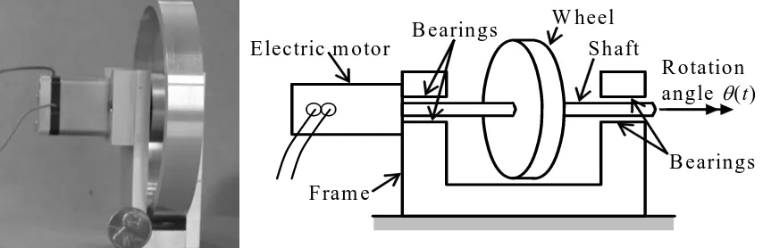
3-3 Reaction wheel: a rotational 1st order system 3-3

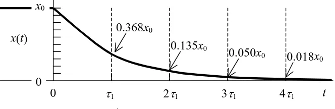
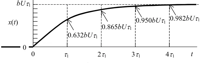
3-4 Simple transient responses of 1st order systems, 1st order time constant

and settling time

3-4

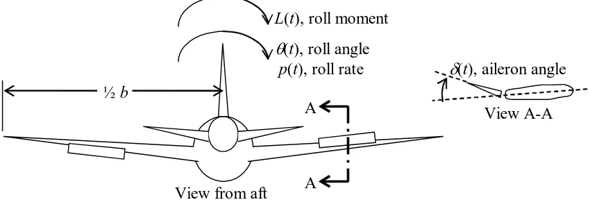
3-5 Aileron-induced rolling of an airplane or missile 3-8

3-6 Translational spring and viscous damper (dashpot) 3-11

3-7 More examples of damped mechanical systems 3-13

Section Title Page

Chapter

4

Frequency response of 1

order systems; transfer function;

general method for derivation of frequency response

4-1 Definition of frequency response 4-1

4-2 Response of a 1st order system to a suddenly applied cosine, cosω t 4-1

4-3 Frequency response of the 1st order damper-spring system 4-4

4-4 Period, frequency, and phase of periodic signals 4-8

4-5 Easy derivation of the complex frequency-response function for

standard stable 1st order systems

4-10

4-6 Transfer function, general definition 4-11

4-7 Frequency-response function from transfer function, general derivation 4-12

4-8 Homework problems for Chapter 4 4-15

Chapter 5

Basic electrical components and circuits

5-1 Introduction 5-1

5-2 Passive components: resistor, capacitor, and inductor 5-1

5-3 Operational amplifier (op-amp) and op-amp circuits 5-9

5-4 RC band-pass filter 5-12

5-5 Homework problems for Chapter 5 5-13

Chapter

6

General time response of 1

order systems by application of

the convolution integral

Section Title Page

6-2 General solution of the standard stable 1st order ODE + IC by

application of the convolution integral

6-2

6-3 Examples of 1st order system response 6-3

6-4 General solution of the standard 1st order problem: an alternate

derivation

6-6

6-5 Numerical algorithm for the general solution of the standard 1st order

problem

6-7

6-6 Homework problems for Chapter 6 6-11

Chapter

7

Undamped 2

order systems: general time response;

undamped vibration

7-1 Standard form for undamped 2nd order systems; natural frequency ωn 7-1

7-2 General solution for output x(t) of undamped 2nd order systems 7-3

7-3 Simple IC response and step response of undamped 2nd order systems 7-4

7-4 Discussion of the physical applicability of step-response solutions 7-6

7-5 Dynamic motion of a mechanical system relative to a non-trivial static

equilibrium position; dynamic free-body diagram

7-7

7-6 Introduction to vibrations of distributed-parameter systems 7-9

7-7 Homework problems for Chapter 7 7-17

Chapter

8

Pulse inputs; Dirac delta function; impulse response;

initial-value theorem; convolution sum

Section Title Page

8-2 Impulse-momentum theorem for a mass particle translating in one

direction

8-2

8-3 Flat impulse 8-3

8-4 Dirac delta function, ideal impulse 8-3

8-5 Ideal impulse response of a standard stable 1st order system 8-5

8-6 Derivation of the initial-value theorem 8-7

8-7 Ideal impulse response of an undamped 2nd order system 8-9

8-8 Ideal impulse response vs. real response of systems 8-10

8-9 Unit-step-response function and unit-impulse-response function (IRF) 8-12

8-10 The convolution integral as a superposition of ideal impulse responses 8-14

8-11 Approximate numerical solutions for 1st and 2nd order LTI systems

based on the convolution sum

8-15

8-12 Homework problems for Chapter 8 8-28

Chapter 9

Damped 2

order systems: general time response

9-1 Homogeneous solutions for damped 2nd order systems; viscous

damping ratio ζ

9-1

9-2 Standard form of ODE for damped 2nd order systems 9-3

9-3 General solution for output x(t) of underdamped 2nd order systems 9-6

9-4 Initial-condition transient response of underdamped 2nd order systems 9-8

9-5 Calculation of viscous damping ratio ζ from free-vibration response 9-9

9-6 Step response of underdamped 2nd order systems 9-12

Section Title Page

9-8 Step-response specifications for underdamped systems 9-14

9-9 Identification of a mass-damper-spring system from measured response

to a short force pulse

9-18

9-10 Deriving response equations for overdamped 2nd order systems 9-20

9-11 Homework problems for Chapter 9 9-23

Chapter

10

2

order systems: frequency response; beating response to

suddenly applied sinusoidal (SAS) excitation

10-1 Frequency response of undamped 2nd order systems; resonance 10-1

10-2 Frequency response of damped 2nd order systems 10-2

10-3 Frequency response of mass-damper-spring systems, and system

identification by sinusoidal vibration testing

10-7

10-4 Frequency-response function of an RC band-pass filter 10-10

10-5 Common frequency-response functions for electrical and

mechanical-structural systems

10-11

10-6 Beating response of 2nd order systems to suddenly applied sinusoidal

excitation

10-14

10-7 Homework problems for Chapter 10 10-19

Chapter

11

Mechanical systems with rigid-body plane translation and

rotation

11-1 Equations of motion for a rigid body in general plane motion 11-1

11-2 Equation of motion for a rigid body in pure plane rotation 11-3

Section Title Page

11-4 Homework problems for Chapter 11 11-13

Chapter

12

Vibration modes of undamped mechanical systems with two

degrees of freedom

12-1 Introduction: undamped mass-spring system 12-1

12-2 Undamped two-mass-two-spring system 12-2

12-3 Vibration modes of an undamped 2-DOF typical-section model of a

wing

12-9

12-4 Homework problems for Chapter 12 12-13

Chapter

13

Laplace block diagrams, and additional background material

for the study of feedback-control systems

13-1 Laplace block diagrams for an RC band-pass filter 13-1

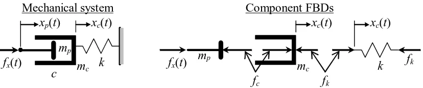
13-2 Laplace block diagram with feedback branches for an m-c-k system

with base excitation

13-2

13-3 Forced response of an m-c-k system with base excitation 13-4

13-4 Homework problems for Chapter 13 13-7

Chapter

14

Introduction to feedback control: output operations for

control of rotational position

14-1 Initial definitions and terminology 14-1

14-2 More definitions, and examples of open-loop control systems 14-2

Section Title Page

14-4 Transfer function of a single closed loop 14-9

14-5 Closed-loop control of rotor position using position feedback plus rate

feedback

14-11

14-6 Comments regarding classical control theory and modern control theory 14-17

14-7 Homework problems for Chapter 14 14-18

Chapter

15

Input-error operations: proportional, integral, and derivative

types of control

15-1 Initial definitions; proportional-integral-derivative (PID) control 15-1

15-2 Examples of proportional (P) and proportional-integral (PI) control 15-2

15-3 Derivation of the final-value theorem 15-12

15-4 Example of proportional-derivative (PD) control 15-13

15-5 Homework problems for Chapter 15 15-16

Chapter

16

Introduction to system stability: time-response criteria

16-1 General time-response stability criterion for linear, time-invariant

systems

16-1

16-2 Stable and unstable PD-controlled-rotor systems 16-6

16-3 Routh’s stability criteria 16-12

16-4 Loci of roots for 2nd order systems 16-18

16-5 Loci of roots for 3rd order systems 16-22

Section Title Page

16-7 Homework problems for Chapter 16 16-34

Chapter

17

Introduction to system stability: frequency-response criteria

17-1 Gain margins, phase margins, and Bode diagrams 17-1

17-2 Nyquist plots 17-9

17-3 The practical effects of an open-loop transfer-function pole at s = 0 +

j0

17-12

17-4 The Nyquist stability criterion 17-15

17-5 Homework problems for Chapter 17 17-23

References

Appendix A: Table and derivations of Laplace transform pairs

A-1 Table of Laplace transform pairs used in this book A-1

A-2 Laplace transform of a ratio of two polynomials, with only simple

poles

A-4

A-3 Derivation of the Laplace transform of a definite integral A-5

A-4 Applications of the Laplace transform of a definite integral A-6

Section Title Page

Appendix B: Notes on work, energy, and power in mechanical

systems and electrical circuits

B-1 Definitions of work and power B-1

B-2 Mechanical work, energy, and power (complementary to Chapter 3) B-2

B-3 Work, energy, and power in electrical circuits (complementary to

Chapter 5)

B-4

B-4 Analogies between an m-c-k mechanical system and an LRC electrical

circuit

B-8

B-5 Hysteresis and dissipation of mechanical energy by damping B-9

Chapter 1

Introduction; examples of 1

and 2

order systems,

time-response analysis and graphing with MATLAB

© 2016 by William L. Hallauer, Jr.

1-1 Introduction

The subject of this book is the dynamic behavior of physical systems, with some

emphasis on simple mechanical and electrical systems representative of or analogous to

those often encountered in aerospace and mechanical engineering. A system, as defined

in this book, is a combination of two or more simple physical elements or components,

these being connected together in such a way that they all influence the dynamic behavior

of the entire system. An element or component, as defined in this book, is usually a

discrete object, such as a mechanical spring or an electrical resistor. This object usually

produces a discrete effect, such as a motion-induced force or a voltage drop. Dynamic

behavior is the variation in time of some physical response quantity of the system, for example, the position of a mass, or the voltage at some location in an electrical circuit.

The general subject of this book is relevant to courses that are offered in most engineering colleges for students who major in aerospace engineering, mechanical engineering, engineering mechanics, ocean engineering or naval architecture, electrical engineering, and chemical engineering. Many of the specific topics addressed within chapters and in homework problems following chapters are relevant especially to the study and practice of aerospace engineering.

1-2 Linear, time-invariant (LTI) systems and ordinary differential equations (ODEs)

We consider physical systems that can be modeled with reasonable engineering

fidelity as linear, time-invariant (LTI) systems. Such a system is represented

mathe-matically by an ordinary differential equation (ODE), or by a set of coupled ODEs, for

which the single independent variable is time, denoted as t. These ODEs are linear, and

they have constant coefficients, so we describe them as linear, time-invariant (LTI), the

same as the systems they represent.2 For example, suppose we denote a dependent

vari-able as x(t), here a general symbol representing some physical dynamic response quantity for which we want to solve. Then an LTI ODE that models an LTI physical system might have the form

) (t u b x a dt dx

=

− (1-1)

1

MATLAB ® is a registered trademark of The MathWorks, Inc.

2

in which a and b are constant multiplying coefficients, and known function u(t) is the ex-citation and is independent of the response.3 In the study of systems, an independent excitation u(t) is often called an input, and a dependent response x(t) is often called an

output.

Hereafter, we will usually employ the common shorthand dot notation for

denot-ing derivatives with respect to time: x

dt dx

&

≡ , x dt

x d

&& ≡ 2 2

, etc., so that Eq. (1-1) can be writ-ten more simply as x&−ax=bu(t).

The linearity of Eq. (1-1) is manifested by the linear appearance of x(t) and all of its derivatives in the ODE. The following are some similar ODEs that are not linear (they are nonlinear) for obvious reasons: x&−ax2 =bu(t); sin(x&)−ax=bu(t); x& −atan(x)

= . Linear ODEs are almost always easier to solve (at least in closed form, i.e., as

equations involving standard functions) than nonlinear ODEs. Moreover, the important

principle of superposition applies to linear ODEs, but not to nonlinear ODEs. An

exam-ple of the application of this princiexam-ple is: let the response to input be , and let

the response to another input be ; if a third input is the sum of multiplied

terms , in which and are constants, then the response to

is . This result is easy to derive just by multiplying two

ODEs such as (1-1) by the constants, then adding the multiplied ODEs. The principle of superposition allows us to solve accurately for the responses of linear systems to any physically realistic inputs. (See Section 8-10 for a derivation of system response to an arbitrary physically realistic input by direct application of superposition.)

) (t u b

3 u

) (

3 t

) (

1 t

u x₁(t) ) x2(t)

1

c c₂

(

2 t

u

) (t

) ( )

( )

(t =c₁u₁ t +c₂u₂ t

) ( )

( _{1 1 2 2}

3 t c x t c x

x = +

u

The time invariance of Eq. (1-1) is manifested by the constant coefficients of x(t) and all of its derivatives in the ODE. ODEs with time-invariant coefficients model the behavior of systems assumed to have physical properties that either remain constant in time or vary so slowly and/or slightly that the variation is negligible for engineering pur-poses. But many practically important systems have time-varying physical properties. For example, a vehicle such as a space shuttle between liftoff and achievement of orbital position has rapidly varying (decreasing) mass as propellant is burned and external fuel tanks and boosters are released. The following is a linear equation somewhat similar to

Eq.(1-1), but with an obviously time-varying coefficient: . The

study of systems with time-varying physical properties is generally more complicated, not fundamental, so only time-invariant systems and ODEs are considered in this book.

) ( )

1 (

3 e 2 x bu t

x&− − − t =

The form of Eq. (1-1), x&−ax=bu(t), is widely regarded as the standard form

for a 1st order LTI ODE, and we will use it as such in this book. Beginning in the next

section, we will study idealized physical systems whose dynamic behaviors are described by equations that are directly analogous to Eq. (1-1). We will express the mathematical

3

constants a and b in terms of specific physical constants. Also, the roles of input u(t) and

output x(t) in Eq. (1-1) will be assumed by some specific physical quantities, such as

force, velocity, voltage, etc., and we will denote them with relevant symbols [often

dif-ferent than u(t) and x(t)] when appropriate.

Although only 1st order ODEs are discussed in this section, we certainly will

en-counter and study systems and ODEs of 2nd and higher orders.

1-3 The mass-damper system: example of 1st order LTI system and ODE

Consider a rigid body of mass m that is constrained to sliding translation x(t) in only one direction, Fig. 1-1. The mass is subjected to an externally applied, arbitrary

force fx(t), and it can slide on a thin, viscous liquid layer such as water or oil. The

vis-cous force acting on the mass due to sliding on the liquid layer is opposite to the direction

of velocity, , and we assume that the magnitude of viscous force is

propor-tional to velocity with constant of proporpropor-tionality c, called the viscous damping constant. Mass m and viscous damping constant c are positive physical quantities.

) ( )

(t x t

v ≡ &

All of the forces

acting on the mass are as shown on the free-body diagram (FBD) of Fig. 1-1.

Idealized physical model

m Liquid layer with viscous

damping constant c

x(t)

fx(t)

Free-body diagram (FBD)

fx(t)

x(t)

cv(t)

Figure 1-1 1st order mass-damper mechanical system

m

Next, we use (from your engineering dynamics course) the FBD of Fig. 1-1 and

Newton’s 2nd law of motion (after English physicist and mathematician Isaac Newton,

1642-1727) for translation in a single direction, to write the equation of motion for the mass:

Σ (Forces)x = mass × (acceleration)x, where (acceleration)x = v dt dv

& = ;

v m v c t

fx( )− = &.

As is customary in writing ODEs, we collect all terms involving the dependent variable and its derivatives on the left-hand side, and put all independent input functions on the right-hand side:

) (t f v c v

ODE (1-2) is clearly linear in the single dependent variable, velocity v(t), and time-invariant, assuming that m and c are constants. The highest derivative of v(t) in the ODE is the first derivative, so this is called a 1st order ODE, and the mass-damper system is called a 1st order system. If fx(t) is defined explicitly, and if we also know some initial condition (IC) of the velocity, v₀ ≡v(t₀) at time t = , then we can, at least in principle, solve ODE (1-2) for velocity v(t) at all times t> . (In this book, we will usually define the initial time as = 0 second.)

0 t 0 t 0

t

Equation (1-2) expressed in the form of the standard 1st order LTI ODE (1-1)

be-comes , where v&−av=bf_x(t) a=−c m and b=1m. Since m and c are positive physi-cal constants, a is clearly negative. This negative polarity is characteristic of most physi-cal systems that we will study; we shall see that it has an important influence on the gen-eral nature of the transient response of systems.

Note that after solving for velocity v(t), we can solve by direct integration another

ODE for position x(t), provided that we know the initial position at time t =

. One systematic method for finding x(t) is based upon the derivative definition: ) ( ₀

0 x t

x ≡ 0

t

ODE: ( ) ( ) v(t)

dt t dx t

x& ≡ =

The following shows careful definite integration of both sides of the ODE, using τ as the “dummy” variable of integration to distinguish it from the upper limit, time t:

∫

∫

= =

=

= t t t

t

d v d

d

dx τ

τ τ

τ

τ τ τ

τ τ

0 0

) ( )

(

⇒

∫

=

= = −

t t

d v t

x t x

τ

τ

τ τ

0

) ( ) ( )

( 0

⇒

∫

=

= +

= t

t d v x t x

τ

τ

τ τ

0

) ( )

( ₀

Another popular method of solution is to find the antiderivative (indefinite integral) of

the ODE and add a constant of integration C, which then must be determined in terms of

the initial condition:

C dt t v t

x( )=

∫

[

∫

]

[

∫

]

⇒ = +

∫

[

∫

]

0

) ( )

( )

(t x0 v t dt v t dt t t

1-4 A short discussion of engineering models

The mass-damper of Fig. 1-1 can be used to represent approximately (i.e., to

model) some actual physical systems. One such system is a surface ship moving over the water under its own propulsion or being pushed/pulled by a tugboat. Another is an auto-mobile hydroplaning on a wet road. You can probably think of other similar real sys-tems. However, it is important for us, as engineers, to recognize that the mass-damper

system is not the actual system, but only an approximate idealized physical model of the

actual system. We are able to derive from this idealized physical model the solvable

mathematical model, which consists of ODE (1-2) and known values for fx(t) and .

The actual physical system, on the other hand, might be so complicated that it cannot be characterized mathematically with absolute precision. For example, the ideal viscous damping model used in the derivation of ODE (1-2) is almost certainly not an exact rep-resentation of the liquid drag forces acting on either a surface ship or a hydroplaning car.

0 v

The same general observation applies for almost any idealized physical model and associated mathematical model developed for engineering purposes: the physical model is, at best, a reasonably accurate approximation of the actual physical system. The fidel-ity of a model usually depends on a number of factors, including system complexfidel-ity, un-certainties, the costs of modeling and mathematical/computational solutions, time con-straints, modeling skills of the engineer, etc.

But a reasonably accurate approximate model often suffices for engineering pur-poses. Engineering systems are usually designed conservatively, with redundancies and factors of safety to compensate for severe overloads, unexpected material flaws, operator error, and the many other unpredictable influences that can arise in the functioning of a system. As engineers, we almost never require 100% accuracy; we are usually satisfied if our mathematical/computational predictions of system behavior are qualitatively correct and are quantitatively within around ±10% (in a general sense) of the actual behavior.

The main point of this discussion is to emphasize that any idealized physical model used for engineering analysis and design is only an approximation of an actual physical system. Moreover, the primary subjects of this book are the fundamental dyna-mic characteristics of idealized physical models, because a great deal of practical experi-ence has shown that these are also the characteristics of many real engineering systems. Therefore, this book does not consider in depth the development of idealized physical models to represent actual systems; rather, we shall focus on deriving mathematical models (mostly ODEs) that describe idealized physical models, and on solving the mathematical equations and exploring the characteristics of the solutions.

1-5 The mass-damper system (continued): example of solving the 1st order LTI ODE for time response, given a pulse excitation and an IC

An input of limited duration, typically called a pulse, is a very common type of

excitation imposed onto systems. For example, when a hammer strikes a nail, the force imposed on the nail by the hammer is a pulse. A real pulse such as hammer impact force is often modeled as a half-sine pulse. Let the force acting on the mass in Fig. 1-1 be the half-sine pulse described by the following figure and Eq. (1-5):

F fx(t)

t

0 0

td

⎪ ⎪ ⎪ ⎩ ⎪⎪ ⎪

⎨ ⎧

<

≤ ≤ ⎟⎟ ⎠ ⎞ ⎜⎜ ⎝ ⎛

=

t t

t t t

t F

t f

d

d d

x

, 0

0 , sin

) (

π

(1-5)

In Eq. (1-5) for fx(t), denotes the pulse duration. The notation will be more

manage-able in this problem if we express the time-varying sinusoid in the form

d t

t

ω

sin , where ω

denotes the circular frequency of oscillation, in radians per second. In this case, clearly

the circular frequency is expressed in terms of the pulse duration as ω =π t_d

v

. Let’s

specify that the initial velocity of the mass at time t = 0 is some known value . The

mathematical statement of the problem for finding the velocity time-history is:

0

ODE: mv&+cv= f_x(t) (1-2, repeated) IC: v(0) = v₀

Find: v(t) for all t > 0.

To solve this problem in closed form, we will use a method with which you

should be familiar from your previous study of ODEs. First, we find the homogeneous

(also called complementary) solution , which is the solution of the homogeneous

ODE, the version of Eq. (1-2) with zero right-hand side: )

(t vh

0

= + _h h cv v

m& (1-6)

A homogeneous LTI ODE always has solutions in time-linear powers of e = 2.71828...

(the base of natural logarithms), with some initially unknown constant coefficients:

t h t Ce

v ( )= λ , in which constants C and λ are unknown at this stage.

0 )

( + =

=

+ t t

t

e C c m e

C c e C

m λ λ λ λ λ

If Ceλt= 0, we get the useless trivial solution vh(t) = 0, so a useful solution requires that

mλ + c = 0, which is known as the characteristic equation of the ODE. Solution of this equation gives the so-called characteristic value, λ=−c m, leading to:

t m c h t Ce

v ( )= −( ) (1-7)

Note that we still have not solved for constant C. We can find C only after we

have determined a particular solution, also known as the non-homogeneous solution

be-cause it is a solution that satisfies the complete ODE (1-2) for the given right-hand side

fx(t). For this problem, we will need two particular solutions, because fx(t) is defined

dif-ferently over two different intervals of time, Eq. (1-5). First, we find a particular solution

valid over the pulse duration, 0 ≤t≤ , for which the ODE is:

) (t

vp td

t F v c v

m&_p + _p = sinω , where ω =π t_d (1-8)

To find a particular that satisfies ODE (1-8), we apply the method of undetermined

coefficients, which entails making an educated guess of the functional character of the solution, using multiplicative coefficients that will be determined by substituting the can-didate solution back into ODE (1-8). The right-hand-side sine function of ODE (1-8) has a finite set of derivatives: the derivative of a sine is a cosine, the derivative of a cosine is

a sine, etc. Therefore, we assume a form of solution consisting of a linear sum of the

function and all of its derivatives: )

(t v_p

t P

t P t

vp( )= 1sinω + 2cosω , with coefficients P1 and P2 undetermined at this stage.

Substitute this candidate solution back into ODE (1-8):

(

) (

)

mω ₁cosω − ₂sinω + ₁sinω + ₂cosω = sinω Collect terms that multiply sinωt andcosωt on both sides of the equation:

(

)

(

)

Functions sinωtandcosωt are linearly independent of each other, which requires that

the left-hand-side and right-hand-side terms multiplying sinωt must equal each other,

and the same for the terms multiplying cosωt, leading to two algebraic equations for the coefficients P1 andP2:

F P m P

The second equation gives P2 =−(mω c)P1, and substituting this into the first equation to

eliminate P₂ leads to:

1 2

2 2

1 and

)

( c P

m P

c m

F c

P ω

ω

− = +

= (1-9)

Rather than write out messy algebraic formulas for all the coefficients in this problem, it is convenient to express all others in terms of P1, as is P2 in Eq. (1-9).

To obtain the complete solution for the pulse duration, 0 ≤ t ≤ , we now

com-bine the homogeneous and particular solutions:

d t

t P

t P e

C t v t v t

v( )= _h( )+ _p( )= −(cm)t + ₁sinω + ₂cosω , for 0 ≤t≤ t_d (1-10) Coefficient C in Eq. (1-10) is still not known; but now, finally, we can apply the initial condition (IC) to determine C:

) 1 ( ) 0 ( ) 1 ( )

0

( v₀ C P₁ P₂

v = = + + ⇒ C=v₀ −P₂ =v₀ +(mω c)P₁ (1-11)

Equations (1-9) through (1-11) describe the velocity response during the pulse duration, 0 ≤t≤ , so we still need to find the post-pulse response, for < t. To do so, we should recognize two facts: (1) fx(t) = 0 for < t; and (2) velocity v(t) cannot

sud-denly change at t = (because acceleration cannot be infinite), rather, velocity must

equal Eq. (1-10) evaluated at t = . Fact 1 means that the ODE for < t is homogene-ous; hence, the particular solution is zero, and we have only a homogeneous solution, but now with a different coefficient, D, than before:

d

t t_d

d t d

t

d

t t_d

t m c e D t

v( )= −( ) , for t_d < t (1-12) To find D, we use Fact 2, which essentially is the IC for t_d < t, and Eq. (1-10):

d d

t m c d

t m c

t P t P e

C t v e

D d _{( )} d _sinω _cosω

2 1

) ( )

( _{= =} − _{+ +}

−

(1-13)

⇒ cmtd d e t v

D= ( ) ( )

⇒ m(t td)

c d e t v t

v( )= ( ) − − , for t_d < t (1-14)

Equation (1-14), with Eq. (1-13) for v( ), combined with Eq. (1-9) and Eq. (1-11) for

coefficients , and C, represents the response for < t. Because mass m and

vis-d t 1

cous damping constant c are positive physical quantities, Eq. (1-14) is a pure exponential decay, which approaches zero as t→∞.

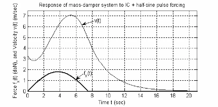
1-6 The mass-damper system (continued): numerical/graphical evaluation of time response using MATLAB

For the mass-damper response solution developed in the previous section, con-sider the following numerical case, with all quantities expressed in SI units: m = 5 kg, c

= 2 N-sec/m, F = 18 N, = 7.5 sec, = 3.3 m/sec. A MATLAB script M-file, named

MATLABdemo11.m, to calculate and graph the response from 0 to 25 seconds is given below. The MATLAB commands are supplemented with explanatory comments, so you should be able to follow and understand the M-file without much difficulty. Writing comments in this manner is good practice for your own programs; comments added while you are writing a computer program are especially helpful if you need to revise or refer back to the program long after you have forgotten the details.

d

t v0

MATLAB script:

%MATLABdemo11.m

%Mass-damper system response to IC + half-sine pulse forcing m=5;c=2; %system mass & viscous damping coefficient, SI units F=18;td=7.5; %half-sine pulse, amplitude (N), pulse duration (sec) vo=3.3; %initial velocity (m/sec)

w=pi/td; %circular frequency of half-sine pulse (rad/sec) t1=0:0.05:td; %time instants for forced response

f1=F*sin(w*t1); %force pulse

P1=c*F/((w*m)^2+c^2);P2=P1*(-w*m/c);C=vo-P2; %constants

v1=C*exp(-c/m*t1)+P1*sin(w*t1)+P2*cos(w*t1);%time series of forced velocity nt1end=length(t1);v2o=v1(nt1end);%initial velocity for post-pulse response t2=td:0.1:25; %time instants for post-pulse unforced response

v2=v2o*exp(-c/m*(t2-td));%time series of post-pulse unforced velocity f2=zeros(1,length(t2)); %null force after pulse

plot(t1,f1/10,'k',t1,v1,'k',t2,f2,'k',t2,v2,'k'),grid,xlabel('Time t (sec)') ylabel('Force f_x(t) (daN), and Velocity v(t) (m/sec)')

title('Response of mass-damper system to IC + half-sine pulse forcing')

To execute in MATLAB an M-file that is stored on a folder (directory) of your com-puter’s hard disk, you must have added that folder to the so-called MATLABpath. In Versions 6 and higher of MATLAB, you can add the folder to the MATLABpath by specifying the folder as the “Current Directory” in the formatting toolbar above the MATLAB command window. The command line below executes the script M-file.

MATLAB command:

>> MATLABdemo11

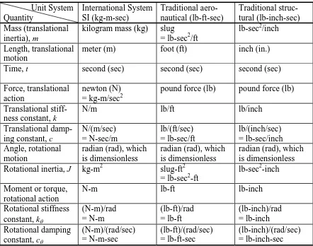
Note that the unit of force “daN” on Fig. 1-2 is a deka-newton, which means 10 newtons. All of the mechanical units used in this book are described in Chapter 3.

Figure 1-2 Excitation and response of a mass-damper system

1-7 Some notes regarding good engineering graphical practice, with reference to Figure 1-2

* Always label both axes, and always include the units of physical quantities.

* Always write an explanatory one-line title. Such a short title cannot explain everything about the graph, but any title you use will almost certainly help the reader to understand the graph.

* It is usually good practice to add grids to a graph. Grids help the reader to perceive values correctly. For example, the grids on Fig. 1-2 show clearly that the peak velocity response is just above 7 m/sec at a little after 5 sec.

* The commands in the script file that specify the densities of computed points are, first,

t1=0:0.05:td while the pulse acts and, second, t2=td:0.1:25 following the pulse. For

example, the first line directs MATLAB to compute the response at 0.05-sec intervals;

then plot(…,t1,v1,'k',…) directs MATLAB to plot small points for those instants, and

dis-continuities). To visualize an extreme example of low point density, suppose that for the mass-damper system you were to compute and plot the velocity response at 4-sec inter-vals; the velocity graph in Fig. 1-2 would consist only of straight lines connecting the computed points at 0, 4, 8, 12, 16, and 20 seconds, which would badly represent the ac-tual response. So always specify high point density on graphs of continuous physical re-sponse. You might not know initially what point density you should use, especially if you are analyzing an unfamiliar system. But try some plausible point density. If your plotted response curve appears unnaturally kinky, then increase the point density appro-priately and run the M-file again. It will cost you nothing more than the little time re-quired to edit and re-run the M-file (or any other graphing computer program).

1-8 Plausibility checks of system response equations and calculations

We all make mistakes in the process of analyzing engineering problems. Most common are mistakes in arithmetic, algebra, calculus, theory, and calculation algorithms (usually computer programming). Also, sometimes we simply use incorrect data. It seems that there are countless ways to make mistakes. Therefore, it is important always to check your mathematical, numerical, and computational operations and results in every way possible. An important type of check for any problem with physical results is the

plausibility check, known more colloquially as reality check and sanity test. Essentially you examine the results to determine if they are physically plausible (believable, credible, reasonable). Do the results make sense physically? A classic example of implausible result that often appears on exam papers in structures courses is the structural deforma-tion on the order of 103 or 106 inches, when it ought to be on the order of 10−3 inches.

To illustrate a plausibility check, let’s examine Fig. 1-2 for the velocity response of the mass-damper system to an initial condition and half-sine pulse excitation. First, the specified initial velocity is = 3.3 m/sec, and the response curve at time t = 0 cor-rectly reflects that initial condition. Next, for about the first half-second of response, the velocity decreases due to viscous drag force cv. But then, as the applied force fx(t)

in-creases, the velocity dips to a local minimum and subsequently increases. Applied force

fx(t) peaks at

0 v

d t

t = 12 = 3.75 sec, and the graph shows that the slope of the velocity curve,

acceleration v, is maximum at about the same time. The velocity itself peaks at a bit past 5 sec. Because velocity is the integral of acceleration (area under the acceleration curve), this lag of the velocity peak behind the force pulse peak is quite plausible. After the ve-locity peaks, it decreases monotonically toward zero as the applied force decreases to

zero at t = = 7.50 sec and remains at zero thereafter. So the entire response, as

de-picted graphically, is physically plausible.

&

d t

1-9 The mass-damper-spring system: example of 2nd order LTI system and ODE

Consider a rigid body of mass m that is constrained to sliding translation x(t) in only one direction, Fig. 1-3. The mass is subjected to an externally applied, arbitrary

force fx(t), and it slides on a thin, viscous, liquid layer that has linear viscous damping

constant c. Additionally, the mass is restrained by a linear spring. The force exerted by the spring on the mass is proportional to translation x(t) relative to the undeformed state of the spring, the constant of proportionality being k. Parameters m, c, and k are positive physical quantities. All of the horizontal forces acting on the mass are shown on the FBD of Fig. 1-3.

Idealized physical model

m

Liquid layer, viscous damping constant c x(t)

fx(t)

Free-body diagram (FBD)

fx(t) x(t)

cv(t)

Figure 1-3 2nd order mass-damper-spring mechanical system

m kx(t)

Linear spring, constant k

From the FBD of Fig. 1-3 and Newton’s 2nd law for translation in a single

direc-tion, we write the equation of motion for the mass:

Σ (Forces)x = mass × (acceleration)x, where (acceleration)x = v&=x&&; v

m kx cv t

fx( )− − = &.

Re-arrange this equation, and add the relationship between x(t) and v(t), x& =v: )

(t f x k v c v

m_&+ + = _x (1-15a)

0

=

−v

x& (1-15b) Equations (1-15a) and (1-15b) are a pair of 1st order ODEs in the dependent variables v(t) and x(t). The two ODEs are said to be coupled, because each equation contains both de-pendent variables and neither equation can be solved indede-pendently of the other. Such a pair of coupled 1st order ODEs is called a 2nd order set of ODEs.

Solving 1st order ODE (1-2) in the single dependent variable v(t) for all times t >

requires knowledge of a single IC, which we previously expressed as .

Simi-larly, solving the coupled pair of 1st order ODEs, Eqs. (1-15a) and (1-15b), in dependent

variables v(t) and x(t) for all times t > , requires a known IC for each of the dependent variables:

0

t v₀ =v(t₀)

) ( )

( _{0 0}

0 v t x t

v ≡ = & and x₀ =x(t₀) (1-16)

In this book, the mathematical problem is expressed in a form different from Eqs. (1-15a) and (1-15b): we eliminate v from (1-15a) by substituting for it from (1-15b) with

and the associated derivative

x

v= & v&=x&&, which gives4 ) (t f x k x c x

m _&&+ _&+ = _x (1-17) ODE (1-17) is clearly linear in the single dependent variable, position x(t), and time-invariant, assuming that m, c, and k are constants. The highest derivative of x(t) in

the ODE is the second derivative, so this is a 2nd order ODE, and the mass-damper-spring

mechanical system is called a 2nd order system. If fx(t) is defined explicitly, and if we also

know ICs (1-16) for both the velocity and the position , then we can, at least

in principle, solve ODE (1-17) for position x(t) at all times t> . We shall study the

re-sponse of 2nd order systems in considerable detail, beginning in Chapter 7, for which the

following section is a preview.

) (t₀

x& x(t₀)

0 t

1-10 The mass-spring system: example of solving a 2nd order LTI ODE for time response

Suppose that we have a system of the type depicted on Fig. 1-3 for which the

damping force, in Eq. (1-17), is negligibly small in comparison with inertial force

and structural force . Figure 1-4

is a photograph of a real system

x c& x

m&& kx

5

with so little damping that, under some circum-stances, we may neglect the damping force. The mass carriage of this system rides back and forth on low-friction lin-ear ball blin-earings, which are enclosed underneath the carriage and not visible in the photograph. The entire length of this system, from the left (fixed) end of the spring, to the rightmost edge of the

mass carriage is 8½ inches (21.6 cm), and each of the three light-colored metal slabs at-tached to the carriage has mass of ½ kilogram.

Figure 1-4 Laboratory mass-spring system

If we may neglect the damping force in a system such as that of Fig. 1-4, then the term cx& drops out of Eq. (1-17), and we are left with the simpler 2nd order ODE,

4

An alternative derivation of ODE (1-17) is presented in Appendix B, Section B-2. The rate of change of system energy is equated with the power supplied to the system.

5

) (t f x k x

m &&+ = x (1-18)

If we know ICs (1-16) and excitation force , then we can solve Eq. (1-18) for x(t).

For future reference, note that mass quantity m and spring stiffness constant k are

intrin-sically positive values. Also, observe that may be applied to the system of Fig. 1-4

through the link visible at the right-hand side of the mass carriage. )

(t f_x

) (t f_x

It will be instructive to determine a time response for this 2nd order mass-spring

(m-k) system, by applying the standard ODE solution procedure described in Section 1-5.

We shall find the complete algebraic solution as the sum of homogeneous and particular

solutions, . Suppose that at time t = 0 the spring is undeformed and

the mass is at rest, so that ICs (1-16) are )

( ) ( )

(t x t x t

x = h + p

0 ) 0

( =

x& and x(0)=0 (1-19)

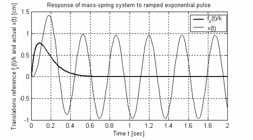
Suppose also that the excitation is a force pulse described by the equation f_x(t) =

) 1 (

)

( ttm

m m t t e

F − ; by applying calculus to this function, you can easily prove that it rises

from zero at t = 0 to the maximum value at time t = , and, thereafter, it gradually

drops back to zero (see Fig. 1-5). In dynamics, a linear function of time such as

m

F t_m

m t t is often called a “ramp” function; since our excitation consists of a declining exponential function multiplied by a ramp function, we call this excitation a “ramped exponential” force pulse.

The homogeneous ODE associated with Eq. (1-18) is mx&&h +kxh =0. We cast

this equation into a familiar form by dividing through by mass m and defining the

posi-tive quantity ω_n2 =k m, giving the ODE

0

2 ₌

+ _{n h}

h x

x&& ω (1-20) The positive root ω_n = k m is called the natural frequency of this m-k system, and ω_n has physical significance that will be discussed below with the final solution. You might remember from your previous study of ODEs, or you can easily verify by substitution in-to Eq. (1-20), that the solution can be expressed as

t C

t C

t

xh( )= 1sinωn + 2cosωn (1-21)

Constants C₁ and C₂ are unknown at this point in the solution process.

) 1 (

)

( ttm

m m p

p kx F t t e x

m && + = − (1-22)

To find a particular that satisfies ODE (1-22), we apply the method of

undeter-mined coefficients, just as in Section 1-5. It is easy to show by successive differentia-tions that all derivatives with respect to time of the function

) (t x_p

) 1 (

)

( ttm

m e t

t − produce only

constant multiples of ( ) (1 ttm) m e t

t − itself, and of _e(1−ttm)_{. Therefore, we seek a particular}

solution that consists of a linear sum of these two functions:

) 1 ( 2 ) 1 (

1( )

)

( ttm ttm

m

p t P t t e Pe

x = − + − (1-23)

We determine constants and by substituting Eq. (1-23) into Eq. (1-22), equating

the coefficients of

1

P P2

) 1 (

)e −

( ttm and

m t

t _e(1−ttm) _{on the two sides of the resulting algebraic}

equation, and then solving for and [homework Problem 1.10(a)]. This process

produces the results

1

P P2

k t m

F P

m m

+

= ₂

1 and 2 1

2

2

2

P k t m

t m P

m m

+

= (1-24)

The complete (but not yet final) solution is

) ( ) ( )

(t x t x t

x = _h + _p = C₁sinω_nt+C₂cosω_nt + ₁( ) (1 ttm) ₂ (1 ttm)

m e Pe

t t

P − + − (1-25)

We now can determine the remaining unknown constants by substituting Eq. (1-25) into

ICs (1-19), and , and solving algebraically for constants and

[homework Problem 1.10(b)]. The results are 0

) 0

( =

x& x(0)=0 C₁ C₂

1 1 2

1 e

t P P C

m n ω

−

= , with

m k n =

ω and C₂ =−P₂e1 (1-26)