Version 1.0
Amy Givler Chapman, Ph.D.
Department of Applied Mathema cs Virginia Military Ins tuteContribu ng Authors
Meagan Herald, Ph.D.
Department of Applied Mathema cs Virginia Military Ins tuteald, Jessica Liber ni
A Note on Using this Text
Thank you for taking your me to read this preface. We will briefly share some key features of this text to (hopefully) improve your experience using it.
For Instructors: How to Use this Text
This text was wri en as a prequel to the APEXCalculus series, a three–volume series on Calculus. This text is not intended to fully prepare students with all of the mathema cal knowledge they need to tackle Calculus, rather it is de-signed to review mathema cal concepts that are o en stumbling blocks in the Calculus sequence. It starts basic and builds to more complex topics. This text is wri en so that each sec on and topic largely stands on its own, making it a good resource for students in Calculus who are struggling with the support-ing mathema cs found in Calculus courses. The topics were chosen based on experience; several instructors in the Applied Mathema cs Department at the Virginia Military Ins tute (VMI) compiled a list of topics that Calculus students commonly struggle with, giving the focus of this text. This allows for a more fo-cused approach; at first glance one of the obvious differences from a standard Pre-Calculus text is its size.
This text, as well as the three volumes of the APEXCalculus series, is available separately for free atwww.apexcalculus.com. All four texts can be purchased as bound volumes for $15 or less per text at Amazon.com.
For Students: How to Read this Text
Many mathema cal texts are wri en in very formal, succinct language. This is a terrific approach if this text is simply used as a resource for someone who is already comfortable with the ideas in the text, but can make it difficult for anyone who is new to the material. This text was wri en in a different fashion. Its goal is to show you mathema cal ideas and concepts explained in an infor-mal style so that your focus is on learning the math, not trying to decipher the sentences.
text, come from the mathema cs as it appears in Calculus. You may no ce that if you use this text as a resource while you are taking Calculus that many of the problems in the text come from problems in Calculus. For example, many of the ques ons asking you to simplify a func on are really unsimplified deriva ves of common func on types, a type of func on with a special meaning that is used in Calculus.
Addi onally, the later sec ons of this text will reinforce many of the ideas of the earlier sec ons. This is en rely on purpose. In Calculus, you will need to use many of these skills in the solu on of a larger problem. The larger problems almost never tell you the names of the skills you will use. This means that you need to iden fy which skills to use and when to use them. To help get you used to these types of problems, this text o en gives you problems that require skills from earlier sec ons, without telling you about it.
Finally, answers (but not solu ons) to all exercises are provided in an ap-pendix at the end of the text. We highly recommend checking your answer to each exercise before moving on to another exercise. This will prevent you from prac cing skills incorrectly and will save you the poten al frustra on of finding out that you have done several problems and made the same mistake on all of them.
Thanks
Many people contributed to this text, in ways small and large. First, thanks are due to the VMI students who first used this text during the Summer Transi-on Program (STP) in 2017 and the VMI cadets who used it during Fall 2017. These students were diligent readers who found many typos and made sug-ges ons that greatly improved the usefulness of the text for students. Second, thanks to Meagan Herald, not only for proofreading the en re text and answer key mul ple mes, but for never complaining about using a work in progress for the basis of VMI’s Pre-Calculus course. Major revisions were made between STP 2017 and Fall 2017 with her help and guidance, including reordering the sec-ons of the text so that exercises and examples did not use concepts that had not been discussed by that point. Meagan also ini ally developed a list of top-ics that formed the basis for those used in this text and well as the Pre-Calculus course at VMI.
beginning.
Finally, thanks are due to my husband Jonathan Chapman who supported me as I worked on this text extra hours outside of the office and who provided me with technical support to streamline the crea on process.
APEX – Affordable Print and Electronic teXts
APEX is a consor um of authors who collaborate to produce high–quality, low–cost textbooks. The current textbook–wri ng paradigm is facing a poten-al revolu on as desktop publishing and electronic formats increase in popular-ity. However, wri ng a good textbook is no easy task, as the me requirements alone are substan al. It takes countless hours of work to produce text, write examples and exercises, edit and publish. Through collabora on, however, the cost to any individual can be lessened, allowing us to create texts that we freely distribute electronically and sell in printed form for an incredibly low cost.
Each text is available as a free .pdf, protected by a Crea ve Commons At-tribu on - Noncommercial 4.0 copyright. That means you can give the .pdf to anyone you like, print it in any form you like, and even edit the original content and redistribute it. If you do the la er, you must clearly reference this work and you cannot sell your edited work for money.
We encourage others to adapt this work to fit their own needs. One might add sec ons that are “missing” or remove sec ons that your students won’t need. The source files can be found atgithub.com/APEXCalculus.
Preface v
Table of Contents vii
1 Numbers and Func ons 1
1.1 Real Numbers . . . 1
1.2 Introduc on to Func ons . . . 18
1.3 Factoring and Expanding . . . 32
1.4 Radicals and Exponents . . . 49
1.5 Logarithms and Exponen al Func ons . . . 55
2 Basic Skills for Calculus 65 2.1 Linear Func ons . . . 65
2.2 Solving Inequali es . . . 71
2.3 Func on Domains . . . 79
2.4 Graphs and Graphing . . . 85
2.5 Comple ng the Square . . . 100
3 Solving and Trigonometric Func ons 107 3.1 Solving for Variables . . . 107
3.2 Intersec ons . . . 116
3.3 Frac ons and Par al Frac ons Decomposi on . . . 123
3.4 Introduc on to Trigonometric Func ons . . . 136
3.5 Trigonometric Func ons and Triangles . . . 143
When we first start learning about numbers, we start with the coun ng num-bers: 1, 2, 3, etc. As we progress, we add in 0 as well as nega ve numbers and then frac ons and non-repea ng decimals. Together, all of these numbers give us the set ofreal numbers, denoted by mathema cians asR, numbers that we can associate with concepts in the real world. These real numbers follow a set of rules that allow us to combine them in certain ways and get an unambiguous answer. Without these rules, it would be impossible to defini vely answer many ques ons about the world that surrounds us.
In this chapter, we will discuss these rules and how they interact. We will see how we can develop our own “rules” that we call func ons. In calculus, you will be manipula ng func ons to answer applica on ques ons such as op miz-ing the volume of a soda can while minimizmiz-ing the material used to make it or compu ng the volume and mass of a small caliber projec le from an engineer-ing drawengineer-ing. However, in order to answer these complicated ques ons, we first need to master the basic set of rules that mathema cians use to manipulate numbers and func ons.
Addi onally, we will learn about some special types of func ons: logarith-mic func ons and exponen al func ons. Logarithlogarith-mic func ons and exponen al func ons are used in many places in calculus and differen al equa ons. Log-arithmic func ons are used in many measurement scales such as the Richter scale that measures the strength of an earthquake and are even used to mea-sure the loudness of sound in decibels. Exponen al func ons are used to de-scribe growth rates, whether it’s the number of animals living in an area or the amount of money in your re rement fund. Because of the varied applica ons you will see in calculus, familiarity with these func ons is a must.
1.1
Real Numbers
We begin our study ofreal numbersby discussing the rules for working with these numbers and combining them in a variety of ways. In elementary school, we typically start by learning basic ways of combining numbers, such as addi on, subtrac on, mul plica on, and division, and later more advanced opera ons like exponents and roots. We will not be reviewing each of these opera ons, but we will discuss how these opera ons interact with each other and how to determine which opera ons need to be completed first in complicated mathe-ma cal expressions.
guideline for which opera ons need to be computed first in complicated expres-sions:
1. Parentheses 2. Exponents
3. Mul plica on/Division 4. Addi on/Subtrac on
O en we learn phrases such as “Please Excuse My Dear Aunt Sally” to help remember the order of these opera ons, but this guideline glosses over a few important details. Let’s take a look at each of the opera ons in more detail.
Parentheses
There are two important details to focus on with parentheses: nes ng and “implied parentheses.” Let’s take a look at an example of nested parentheses first:
Example 1 Nested Parentheses Evaluate
2×(3+ (4×2)). (1.1)
Solu on Here we see a set of parentheses “nested” inside of a sec-ond set of parentheses. When we see this, we want to start with the inside set of parentheses first:
2×(3+ (4×2)) =2×(3+ (8)) (1.2) Once we simplify the inside set of parentheses to where they contain only a sin-gle number, we can drop them. Then, it’s me to start on the next parentheses layer:
2×(3+ (8)) =2×(3+8) =2×(11) =22
(1.3)
This gives our final answer:
2×(3+ (4×2)) =22
brackets, “[” and “]”. This can make it a bit easier to see where the parenthe-ses/brackets start and where they end. Let’s look at an example:
Example 2 Alterna ng Parentheses and Brackets Evaluate
(2+ (3×(4+ (2−1))−1)) +2. (1.4)
Solu on
(2+ (3×(4+ (2−1))−1)) +2= [2+ (3×[4+ (2−1)]−1)] +2
= [2+ (3×[4+ (1)]−1)] +2
= [2+ (3×[4+1]−1)] +2
= [2+ (3×[5]−1)] +2
= [2+ (3×5−1)] +2
= [2+ (15−1)] +2
= [2+ (14)] +2
= [2+14] +2
= [16] +2
=16+2=18
(1.5)
We started by finding the very inside set of parentheses:(2−1). The next layer of parentheses we changed to brackets:[4+ (2−1)]. We con nued alter-na ng between parentheses and brackets un l we had found all layers. As be-fore, we started with evalua ng the inside parentheses first:(2−1) = (1) =1. The next layer was brackets: [4+1] = [5] = 5. Next, we had more paren-theses: (3×5−1) = (15−1) = (14) = 14. Then, we had our final layer:
[2+14] +2= [16] +2=16+2=18. This gives our final answer:
(2+ (3×(4+ (2−1))−1)) +2=18
When you are working these types of problems by hand, you can also make the parentheses bigger as you move out from the center:
(2+ (3×(4+ (2−1))−1)) +2=
[ 2+
(
3×[4+ (2−1)]−1)]+2
There’s one more thing that we have to be careful about with parentheses, and that is “implied” parenthesis. Implied parentheses are an easy way to run into trouble, par cularly if you are using a calculator to help you evaluate an expression. So what are implied parentheses? They are parentheses that aren’t necessarily wri en down, but are implied. For example, in a frac on, there is a set of implied parentheses around the numerator and a set of implied paren-theses around the denominator:
3+4 2+5=
(3+4)
(2+5) (1.6)
You will almost never see the second form wri en down, however the first form can you get into trouble if you are using a calculator. If you enter 3+4÷2+5 on a calculator, it will first do the division and then the two addi ons since it can only follow the order of opera ons (listed earlier). This would give you an answer of 10. However, the work to find the actual answer is shown below.
Example 3 Implied Parentheses in a Frac on Evaluate the expression in (1.6).
Solu on First, let’s go back and find (1.6). You may have no ced that the frac ons above have (1.6) next to them on the right side of the page. This tells us that (1.6) is referring to this expression. Now that we know what we are looking at, let’s evaluate it:
3+4 2+5=
(3+4) (2+5) = (7)
(7) = 7
7
=1
(1.7)
This reflects what we would get on a calculator if we entered(3+4)÷(2+5), giving us our final answer:
3+4 2+5 =1
As you can see, leaving off the implied parentheses dras cally changes our answer. Another place we can have implied parentheses is under root
Example 4 Implied Parenthesis Under a Square Root
Evaluate √
12×3−20 .
Solu on
√
12×3−20=√(12×3)−20
=√(36)−20
=6−20
=−14
(1.8)
This gives our final answer:
√
12×3−20=−14
Most calculators will display √(when you press the square root bu on; no ce that this gives you the opening parenthesis, but not the closing paren-thesis. Be sure to put the closing parenthesis in the correct spot. If you leave it off, the calculator assumes that everything a er√(is under the root oth-erwise. This also applies to other kinds of roots, like cube roots. In the ex-pression in Example 4, without a closing parenthesis, a calculator would give us√(12×3−20=√(36−20=√(16=4.
We’ll see another example of a common issue with implied parentheses in the next sec on.
Exponents
With exponents, we have to be careful to only apply the exponent to the term immediately before it.
Example 5 Applying an Exponent Evaluate
2+33 .
Solu on
2+33 =2+27
No ce we only cubed the 3 and not the expression 2+3, giving us a final answer of
2+33=29
This looks rela vely straight-forward, but there’s a special case where it’s easy to get confused, and it relates to implied parentheses.
Example 6 Applying an Exponent When there is a Nega ve Evaluate
−42 .
Solu on
−42 =−(42) =−(16) =−16
(1.10)
Here, our final answer is
−42=−16
No ce where we placed the implied parenthesis in the problem. Since ex-ponents only apply to the term immediately before them, only the 4 is squared, not−4. Taking the extra step to include these implied parentheses will help re-inforce this concept for you; it forces you to make a clear choice to show how the exponent is being applied. If we wanted to square−4, we would write(−4)2
instead of−42.
Note that we don’t take this to the extreme; 122s ll means “take 12 and square it,” rather than 1×(22).
It’s also important to note that all root opera ons, like square roots, count as exponents, and should be done a er parentheses but before mul plica on and division.
Mul plica on and Division
and division to be on the same level, meaning that one does not take prece-dence over the other. This means you should not doallmul plica on steps and thenalldivision steps. Instead, you should do mul plica on/division from le to right.
Example 7 Mul plica on/Division: Le to Right Evaluate
6÷2×3+1×8÷4
Solu on
6÷2×3+1×8÷4=3×3+1×8÷4
=9+1×8÷4
=9+8÷4
=9+2
=11
(1.11)
Since this expression doesn’t have any parentheses or exponents, we look for mul plica on or division, star ng on the le . First, we find 6÷2, which gives 3. Next, we have 3×3, giving 9. The next opera on is an addi on, so we skip it un l we have no more mul plica on or division. That means that we have 1×8 = 8 next. Our last step at this level is 8÷4 = 2. Now, we only have addi on le : 9+2=11. Our final answer is
6÷2×3+1×8÷4=11
Note that we get a different, incorrect, answer of 3 if we do all the mul pli-ca on first and then all the division.
Addi on and Subtrac on
Just like with mul plica on and division, addi on and subtrac on are on the same level and should be performed from le to right:
Example 8 Addi on/Subtrac on: Le to Right Evaluate
Solu on
1−3+6=−2+6
=4 (1.12)
By doing addi on and subtrac on on the same level, from le to right, we get a final answer of
1−3+6=4
Again, note that if we do all the addi on and then all the subtrac on, we get an incorrect answer of−8.
Summary: Order of Opera ons
Now that we’ve refined some of the ideas about the order of opera ons, let’s summarize what we have:
1. Parentheses (including implied parentheses)
2. Exponents
3. Mul plica on/Division (le to right)
4. Addi on/Subtrac on (le to right)
Let’s walk through one example that uses all of our rules.
Example 9 Order of Opera ons Evaluate
−22+√6−2−2(8÷2×(1+1))
−22+√6−2−2(8÷2×(1+1))= We have a bit of everything here, so let’s write down any implied paren-theses first.
=−22+√(6−2)−2(8÷2×(1+1)) We have nested parentheses on the far right, so let’s work on the inside set.
=−22+√(6−2)−2(8÷2×2) There aren’t any more nested paren-theses, so let’s work on the set of parentheses on the far le .
=−22+√4−2(8÷2×2) Now, we’ll work on the other set of parentheses. This set only has mul-plica on and division, so we’ll work from le to right inside of the paren-theses.
=−22+√4−2(4×2) Now, we’ll complete that set of paren-theses.
=−22+√4−2(8) Let’s rewrite slightly to completely get rid of all parentheses.
=−22+√4−2×8 Now, we’ll work on exponents, from le to right.
=−4+√4−2×8 We only squared 2, and not −2. Square roots are really exponents, so we’ll take care of that next.
=−4+2−2×8 We’re done with exponents; me for mul plica on/division.
=−4+2−16 Now, only addi on and subtrac on are le , so we’ll work from le to right.
=−2−16 Almost there!
=−18
Our final answer is
−22+√6−2−2(8÷2×(1+1)) =−18
Computa ons with Ra onal Numbers
Ra onal numbersare real numbers that can be wri en as a frac on, such as 1
2, 5 4, and−
2
3. You may no ce that 5
animproper frac on. It’s called improper because the value in the numerator, 5, is bigger than the number in the denominator, 4. O en, students are taught to write these improper frac ons as mixed numbers: 54 = 114. This does help give a quick es mate of the value; we can quickly see that it is between 1 and 2. However, wri ng as a mixed number can make computa ons more difficult and can lead to some confusion when working with complicated expressions; it may be temp ng to see 11
4as 1× 1
4 rather than 5
4. For this reason, we will leave all improper frac ons as improper frac ons.
With frac ons, mul plica on and exponents are two of the easier opera-ons to work with, while addi on and subtrac on are more complicated. Let’s start by looking at how to work with mul plica on of frac ons.
Example 10 Mul plica on of Frac ons Evaluate
1 4×
2 3×2
Solu on With mul plica on of frac ons, we will work just like we do with any other type of real number and mul ply from le to right. When mul-plying two frac ons together, we will mul ply their numerators together (the tops) and we will mul ply the denominators together (the bo oms).
1 4×
2 3×2=
1×2 4×3×2
= 2
12 ×2
=1
6×2
=1
6× 2 1
=1×2
6×1
=2
6
=1
3
A er each step, we look to see if we can simplify any frac ons. A er the first mul plica on, we get 2
12. Both 2 and 12 have 2 as a factor (are both divisible by 2), so we can simplify by dividing each by 2, giving us1
6. Before doing the second mul plica on, we transform the whole number, 2, into a frac on by wri ng it as 21. Then, we can compute the mul plica on of the two frac ons, giving us
2
1 4×
2 3×2=
1 3
Next, let’s look at exponen a on of a frac on.
Example 11 Exponen a on of a Frac on
Evaluate (
1+2 5
)2
Solu on With exponen a on, we need to apply the exponent to both the numerator and the denominator. This gives
( 1+2
5 )2
=
(
(1+2) (5)
)2
=
(
(3) (5)
)2
=
( 3 5
)2
= 3
2
52
= 9
25
No ce that we were careful to include the implied parentheses around the numerator and around the denominator. This helps to guarantee that we are correctly following the order of opera ons by working inside of any parentheses first, before applying the exponent. We can’t simplify our frac on at any point since 3 and 5 do not share any factors. This gives us our final answer of
( 1+2
5 )2
= 9
With division of frac ons, we will build off of mul plica on. For example, if we want to divide a number by 2, we know that we could instead mul ply it by
1
2because dividing something into two equal pieces is the same as spli ng it in half. These numbers arereciprocals; 2 can be wri en as 21 and if we flip it, we get 1
2, its reciprocal. This works for any frac ons; if we want to divide by 5 6, we can instead mul ply by its reciprocal,6
5.
Addi on and subtrac on of frac ons can be a bit more complicated. With a frac on, we can think of working with pieces of a whole. The denominator tells us how many pieces we split the item into, and the numerator tells us how many pieces we are using. For example,3
4tells us that we split the item into 4 pieces and are using 3 of them. In order to add or subtract frac ons, we need to work with pieces that are all the same size, so our first step will be ge ng a common denominator. We will do this by mul plying by 1 in a sneaky way. Mul plying by 1 doesn’t change the meaning of our expression, but it will allow us to make sure all of our pieces are the same size.
Example 12 Addi on and Subtrac on of Frac ons Evaluate 1 2− 1 3+ 1 4
Solu on Since we only have addi on and subtrac on, we will work from le to right. This means that our first step is to subtract 13 from 12. The denominators are different, so we don’t yet have pieces that are all the same size. To make sure our pieces are all the same size, we will mul ply each term by 1; we will mul ply1
2by 3
3 and we will mul ply 1 3 by
2
2. Since we are mul plying by the “missing” factor for each, both will have the same denominator. Once they have the same denominator, we can combine the numerators:
1 2− 1 3+ 1 4 = 1 2× 3 3− 1 3× 2 2+ 1 4 =3 6− 2 6+ 1 4
=3−2
= 2
12+ 3 12
= 2+3
12
= 5
12
A er combining the first two frac ons, we had to find a common denomina-tor for the remaining two frac ons. Here, we found the smallest possible com-mon denominator. We did this by looking at each denominator and factoring them. The first denominator, 6, has 2 and 3 as factors; the second denominator, 4 has 2 as a repeated factor since 4=2×2. These means our common denom-inator needed to have 3 as a factor and 2 as a double factor: 3×2×2=12. We don’t have to find the smallest common denominator, but it o en keeps the numbers more manageable. We could have instead done:
1 6+ 1 4 = 1 6× 4 4+ 1 4× 6 6 = 4 24 + 6 24
=4+6
24
=10
24
= 5
12 We s ll end up with the same final answer:
1 2− 1 3+ 1 4 = 5 12
Like frac ons, decimals can also be difficult to work with. Note that all re-pea ng decimals and all termina ng decimals can be wri en as frac ons: 0.333=
1
3and 2.1=2+ 1 10= 20 10+ 1 10 = 21
of digits a er it. For example,
1.2
× 1.1 5 6 0 1 2 1 2 1.3 8 0
Because 1.2 has one digit a er the decimal place and 1.15 has 2 digits a er the decimal place, we need a total of 1+2=3 digits a er the decimal place in our final answer, giving us 1.380, or 1.38. It is important to note that we placed the decimal point before dropping the zero on the end; our final answer would have quite a different meaning otherwise.
Computa ons with Units
So far, we have only looked at examples without any context to them. How-ever, in calculus you will see many problems that are based on a real world problem. These types of problems will come with units, whether the problem focuses on lengths, me, volume, or area. With these problems, it is important to include units as part of your answer. When working with units, you first need to make sure all units are consistent; for example, if you are finding the area of a square and one side is measured in feet and the other side in inches, you will need to convert so that both sides have the same units. You could use measure-ments that are both in feet or both in inches, either will give you a meaningful answer. Let’s look at a few examples.
Example 13 Determining Volume
Determine the volume of a rectangular solid that has a width of 8 inches, a height of 3 inches, and a length of 0.5 feet.
Solu on First, we need to get all of our measurements in the same units. Since two of the dimensions are given in inches, we will start by conver ng the third dimension into inches as well. Since there are 12 inches in a foot, we get
0.5 ×12 in
1 =
0.5×12 × in 1
=6 × in
1
=6 in
simplify ×in as in. This means that we know our rectangular solid is 8 inches wide, 3 inches tall, and 6 inches long. The volume is then
V= (8 in)×(3 in)×(6 in) = (8×3×6)×(in× in× in) = (24×6)×(in× in× in) =144 in3
Since all three measurements are in inches and are being mul plied, we end up with units of inches cubed, giving us a final answer of
V=144 in3
Units can also give you hints as to how a number is calculated. For instance, the speed of a car is o en measured in mph, or miles per hour. We write these units in frac on form asmiles
hour, which tells us that in our computa ons we should be dividing a distance by a me. Some mes, however, a problem will start with units, but the final answer will have no units, meaning it is unitless. We will run across examples of this when we discuss trigonometric func ons. Trigonomet-ric func ons can be calculated as a ra o of side lengths of a right triangle. For example, in a right triangle with a leg of length 3 inches and a hypotenuse of 5 inches, the ra o of the leg length to the hypotenuse length is 3 in5 in = 35. Since both sides are measured in inches, the units cancel when we calculate the ra o. We would see the same final answer if the triangle had a leg of 3 miles and a hypotenuse of 4 miles; they are similar triangles, so the ra os are the same.
Exercises 1.1
Terms and Concepts
1. In your own words, what does “mul plica on and division are on the same level” mean?
2. In an expression with both addi on and mul plica on, which opera on do you complete first?
3. In your own words, what is meant by “implied parenthe-ses”? Provide an example.
4. T/F: In an expression with only addi on and subtrac on re-maining, you must complete all of the addi on before start-ing the subtrac on. Explain.
5. T/F: In the expression−22, only “2” is squared, not “−2.”
Explain.
Problems
In exercises 6 – 15, simplify the given expressions.
6. −2(11−5)÷3+23 7. 3 5+ 2 3÷ 5 6 8. ( 2 3 )2 −1 6
9. (13+7)÷4−32 10.
( 5−1
2 )3
11. (2)(−2)÷1
2
12. 2−4(3−5) 6−7+3 −
√ 25−9
13. √
22+32+5
2−(−1)3 −2+6
minutes at the same pace. What is the distance between her current loca on and her home?
17. The Reynold’s number, which helps iden fy whether or not a fluid flow is turbulent, is given byRe=ρuDµ . Ifρ,u, andD are held constant whileµincreases, doesReincrease, de-crease, or stay the same?
18. Consider a square-based box whose height is twice the length of the base of the side. If the length of the square base is 3 , what is the volume of the box? (Don’t forget your units!)
19. The velocity of periodic waves, v, is given by v = λf whereλis the length of the waves andfis the frequency of the waves. If the wavelength is held constant while the frequency is tripled, what happens to the velocity of the waves? Be as descrip ve as possible.
20. The capacitance,C, of a parallel plate capacitor is given by C= kε0A
d wheredis the distance between the plates. Ifk, ε0, andAare held constant while the distance between the
plates decreases, does the capacitance increase, decrease, or stay the same?
21. Consider a square-based box whose height is half the length of the sides for the base. If the surface area of the base is 16 2, what is the volume of the box?
In exercises 22 – 25, evaluate the given work for correctness. Is the final answer correct? If not, describe the error(s) in the solu on.
22.
12÷6×4−(3−4)2=12÷6×4−(−1)2 =12÷6×4+1
=12÷24+1
= 1
2+1
= 3
2−2(6+3)+ 64+36= 2−2(6+3)+ 64+36 = 2−2
2−2(9) +
√ 64+36
= 2−2
2−2(9) +8+6 = 2−2
2−18+8+6
= 0
−16+14
=14
25.
(−3+1)(2(−3))−((−3)2−3)(1) (−3+1)2 =
(−3+1)(2(−3))−((−3)2−3)(1) (−2)2
= (−2)(−6)−((−3)
2−3)(1)
(−2)2
= (−2)(−6)−(9−3)(1) (−2)2
= (−2)(−6)−(6)(1)
4
= −12−6
4
= −18
4
= −9
1.2 Introduc on to Func ons
This sec on introduces ideas and nota on for func ons. Much of the work in calculus relies heavily on understanding the meaning of a func on and a proper understanding of func on nota on. Here we’ll talk about these ideas and work through several examples involving func on nota on and how they relate to calculus.
What is a Func on?
In mathema cs, we look for pa erns to help explain the world around us. Mathema cians o en use func ons to express these pa erns succinctly. For example, we learn in geometry that the area of a square with sides of length 2 in is 2×2= 4 in2. Similarly, if the square has sides of length 3 in, it’s area is 3×3=9 in2. This shows us a pa ern for determining the area of a square: if we know the side length, we simply mul ply the side length by itself to get the area. Rather than wri ng out what this rule looks like for all sorts of different side lengths, we can express the pa ern as a func on:
A(x) =x×x
=x2 (1.13)
This func on tells us that the area of a square with sides of lengthxhas an area ofx2. This is a lot more compact than wri ng out a table with all sorts of different side lengths and areas.
Func on Nota on
Here we say thatxis theinputof the func onA(x)(read as “Aofx”), and that
x2is the correspondingoutput. No ce that since we get to choose the “name” of the func on,A, we used something that has some meaning for our example; our func on gives us area, so calling the func onAmakes that clearer than if we had chosen something likel(x), where you might be tempted to thinklfor length.
Mathema cians will o en use le ers likef,g, andhto name their func ons, but you can name your func ons anyway you like. In fact, some func ons that you may already be familiar with have longer names, like sin for the sine func-on or cos for the cosine func func-on. Similarly, mathema cians will o en usexto represent the input of the func on, but you can choose any name you want. In our example above, we could uselas our input to stand for “length”, giving us
O en, mathema cians will use “the func onA” and “the func onA(x)” in-terchangeably. Both tell us to use the same rule that is shown in (1.13), but the second gives us an added bit of informa on; it tells us that for the func onA,xis our input variable. For our example func on, this informa on isn’t par cularly useful because the only le er on the right side of our func on isx, but some func ons will have other le ers that aren’t input variables. We’ll run into this fairly o en in calculus. For example, suppose we want to know the height of a ball that has been thrown into the air. Physics (and calculus) gives us a func on for this:
h(t) =h0+v0t+ 1 2at
2 (1.14)
Since the le side hash(t), we know that tis our input variable, but we have lots of other le ers on the right side. These le ers all have meaning for this problem: h0is the ini al height of the ball,v0is the velocity it was thrown at, andais the accelera on due to gravity. While they all have meaning and can change based on the par cular instance of a ball being thrown, they are consideredparametersof the func on, and not input variables. Why? Well, as soon as the ball is thrown,h0,v0, andawon’t change for that ball. Only the me the ball has been in the air changes; the ball has a different height a er
t =2000 seconds than it did a er onlyt =2 seconds. Therefore, onlytis an input variable for this func on. While it might not seem like a big deal to writeA
instead ofA(x), we can see that wri nghinstead ofh(t)could lead to confusion, so it’s good to be careful and include that input variable when it’s not perfectly clear.
Evalua ng a Func on
Now that we are familiar with why we use func ons let’s look at how to evaluate a func on. We’ll start with evalua ng a func on for a single value.
Example 14 Evalua ng a Func on at a Point Determine the value off(−2)iff(x) =x2+4x−10.
Solu on First, we no ce that the le side tells us that our input is
x. Since we want to determine the value off(−2), we’ll replace everyxon the right side with(−2).
f(−2) = (−2)2+4(−2)−10
= (4) +4(−2)−10
=4−8−10=−14
(1.15)
f(−2) =−14
It’s good to no ce that the ques on in Example 14 can be wri en in several different ways. All of the following require the same work, but are worded in slightly different ways:
• Determine the value off(−2)
• Determine the value off(x)forx=−2 • Evaluatef(−2)
• Evaluatefat−2
There are probably more ways to ask this ques on, but these are some of the most common ones. Let’s look at an example where the func on has pa-rameters.
Example 15 Evalua ng a Func on with Parameters
Using the height formula in equa on (1.14), determine the height of a ball 5 seconds a er it was thrown.
Solu on First, let’s make sure we have the correct equa on. The (1.14) label is next toh(t) = h0 +v0t+ 12at2, so that tells us we are work-ing with that func on. The le side tells us thattis our input variable since the func on is calledh(t). That means we need to subs tute(5)forteverywheret
appears in the func on:
h(5) =h0+v0(5) + 1 2a(5)
2
=h0+5v0+ 1 2a(25)
=h0+5v0+ 25
2a
h(5) =h0+5v0+ 25
2a
No ce that in Example 14, we replacedxnot just with−2, but with(−2)
and in Example 15 we replacedtwith(5). This helps in a couple of ways. First, it makes sure we don’t miss any implied parentheses when we squarexin Example 14. Second, it makes sure we replacexandtwith theen reinput. This becomes very important in calculus. In differen al calculus, you will spend a lot of me looking at how quickly func on outputs change when the input only changes a ny bit. You will do this by looking at adifference quo entfor the func on. The general form of difference quo ent for the func onf(x)that you will use is:
f(x+h)−f(x)
h (1.16)
No ce that the numerator starts withf(x+h). This means that everyxon the right side needs to be replaces withx +h. Here, the parentheses make a big difference even with a simple func on likep(x) = x2. If we include the parentheses, we get that
p(x+h) = (x+h)2
= (x+h)×(x+h) =x2+2xh+h2
(1.17)
However, if we don’t include the parentheses, we would getx+h2, which is a very different (and incorrect) answer. Let’s look at an example of finding a difference quo ent for a more complicated func on.
Example 16 Finding a Difference Quo ent Find the difference quo ent forg(t) =2t2−3t+1
ofx, buthwill s ll beh. So, our difference quo ent will look like
g(t+h)−g(t)
h =
[
2(t+h)2−3(t+h) +1]−[2t2−3t+1]
h
=
[
2(t2+2th+h2)−3(t+h) +1]−[2t2−3t+1]
h
=
[
2t2+4th+2h2−3t−3h+1]−[2t2−3t+1]
h
=2t
2+4th+2h2−3t−3h+1−[2t2−3t+1]
h
=2t
2+4th+2h2−3t−3h+1−2t2+3t−1
h
=4th+2h
2−3h
h
=4t+2h−3
There are a few important things to no ce here. First, when we replacedt
with(t+h)in the first term, we included those parentheses to make sure we used the whole input. Second, from line 3 to line 5, we dropped all parentheses; when we did this we made sure to distribute the nega ve to everything inside the second set of parentheses, and not just the first term. We end up with a final answer of
g(t+h)−g(t)
h =4t+2h−3
Common Types of Func ons
There are several different types of func ons that get use commonly in cal-culus. In this sec on, we’ll briefly describe each. Later, we’ll talk about how we can combine these in different ways, what types of inputs these func ons can take, and what their graphs look like.
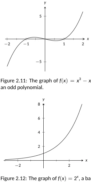
Power Func ons
Apower func onis any func on that involves a variable raised to a power:
Here, the le side tells us thatxis the variable;aandbare parameters that can be any real numbers. Becauseaandbcan be anything, this is a very general func on type meaning that the proper es of the func on can be very different based on these values ofaandb.
Amonomialis a special type of power func on wherebis a non-nega ve integer; this meansbcan be 0, 1, 2, 3, etc. We callbthedegreeof the func on.
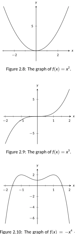
f(x) = 2xhas degree 1,g(x) = 45x13has degree 13, andh(x) = 12 = 12x0 has degree 0. Later, we’ll see that the degree helps us to quickly determine the shape of the func on when we graph it.
If we take one or more monomials and add them together, we get a polyno-mial. That means thatf(x) =2x,g(x) =45x13, andh(x) =12=12x0are not only monomials, but also polynomials, and if we add them all together we get a new polynomial:p(x) =45x13+2x+12. We could get a different polynomial by taking the difference (subtrac ng) them:q(x) =−45x13−2x−12. There are many more polynomials we could make from the three func ons with various combina ons of addi on and subtrac on.
Tradi onally, polynomials are wri en with the highest degree monomial first because for big values ofxit becomes the most important term. The highest degree monomial also tells us the degree of the polynomial:p(x)andq(x)both have degree 13. If the degree of the polynomial is 3, like withr(θ) = 4θ3 +
2θ2−5θ+2, we can call it acubicfunc on, and if the degree is 2, we call it a
quadra cfunc on. If the degree is 1, like withn(t) =5t−2, we simply call it alinearfunc on, and if the degree is 0, we say it’s aconstantfunc on. These four all have special names because they get used very o en in mathema cs.
Root Func ons
Later, we’ll talk more about the importance of root func ons, but for now we’ll focus on what they look line in their general form. Arootfunc on is any func on that looks likef(x) =x1/nwherenis a natural number (a posi ve
inte-ger, or coun ng number like 1, 2, 3, 4, etc.). This means that root func ons are a special type of power func on. The most commonly used root func on is the square root func on,f(x) = x1/2. You’ve most likely seen this wri en in a dif-ferent form:f(x) =√x. There are many other root func ons like the cube root func on (g(x) =x1/3 =√3x) and the fourth root func on (h(x) =x1/4 =√4x).
Exponen al Func ons
Exponen alfunc ons have the formf(x) =bx, withb>0 andb̸=1. No ce
that like a power func on, an exponen al func on involves an exponent, but there is a big difference. For a power func on, the input variable,xis the base with a parameter as the exponent. For an exponen al func on, the roles are swapped: the base is a parameter and the input variable is the exponent.
Logarithmic Func ons
Logarithms, orlogarithmicfunc ons are quite important in many applica-ons of calculus because each logarithmic func on is the inverse of an exponen-al func on. They have the formf(x) =logb(x). Just like with exponen als, we
needb > 0 andb ̸= 1. There are two very commonly used logarithms. The first is log10(10), read as “log base 10 ofx.” Some mes you will see this writ-ten as just log(x)instead of log10(x). The second commonly used logarithm is loge(x), “log baseeofx”, also know as the natural logarithm (commonly wri en
as ln(x)).
Trigonometric Func ons
Trigonometricfunc ons are func ons that relate the angles of a triangle to the length of the sides in that triangle. They can also be used to describe many natural phenomena like waves (sound, light, and water waves) and harmonic mo on (mo on that repeats the same pa ern over and over, also know as cyclic mo on). The trigonometric func ons that are most commonly used are sine (sin(x)), cosine (cos(x)), and tangent (tan(x)). We’ll talk about these func ons and their applica on more later in this text.
Combining Func ons
While each of these func on types has its own set of special uses, o en combina ons of these func ons are needed to accurately model events. For this sec on, we will use three different func ons to help provide examples of how we can combine and modify func ons:
f(x) =3x2 (1.19)
g(x) =x−4 (1.20)
h(x) =√x+6 (1.21)
deriva ve of the func on. This text will not cover deriva ves, but they are one of the most important topics in calculus, so being able to recognize these com-bina on methods will be quite useful in calculus.
Scalar Mul ples of Func ons
The first way we can modify func ons is withscalar mul plica on. This sim-ply means mul sim-plying the func on by a constant (a number). For example,
• 4f(x) =4(3x2) =12x2; • 4g(x) =4(x−4) =4x−16; • 4h(x) =4(√x+6) =4√x+24.
There’s nothing special about the number 4, we could mul ply by anything: nega ve numbers, posi ve numbers, whole numbers, frac ons, decimals, or even zero (even though that would make for a pre y boring result). No ce that for each of these we used parenthesis around the whole func on when we mul-plied. This makes sure that we really mul plied the en re func on by 4, and not just part of the func on. This is par cularly important withg(x)andh(x)
since they each had two terms already and we had to distribute the 4 to both terms.
Sums and Differences of Func ons
One way to combine func ons is to add them (sums) or subtract them (dif-ferences) from each other. For example, the sum off(x)andg(x)isf(x)+g(x) =
3x2+x−4. Sums are nice to work with for many reasons; mathema cians use sums of func ons to get be er and be er approxima ons when working with complicated data, and with sums order doesn’t change the result. If we did
g(x) +f(x)instead off(x) +g(x), we getg(x) +f(x) =x−4+3x2; if we rear-range terms so that the highest degree comes first, we get 3x2+x−4 which is exactly the same asf(x) +g(x).
With differences, we have to be a li le more careful because the order will make a difference. Let’s take a look:
• f(x)−g(x) =3x2−(x−4) =3x2−x+4
• g(x)−f(x) =x−4−(3x2) =x−4−3x2=−3x2+x−4
it really involves mul plying it by−1 and we want to make sure we distribute that nega ve to the en re func on.
With both sums and differences, we can use as many func ons as we want:
f(x)−h(x)−g(x) =3x2−(x−4)−(√x+6) =3x2−x+4−√x−6=3x2−x−√x−2 We can also mix between addi on and subtrac on:
h(x) +g(x)−f(x) =√x+6+x−4−(3x2) =−3x2+x+√x+2
Products of Func ons
Another way of combining func ons is through products (mul plica on) of func ons. Like with sums of func ons, order doesn’t make a difference, so
f(x)g(x) = g(x)f(x). We won’t show the details here, but try to verify it on your own. (Note: it is common for college level mathema cs textbooks to state a property like this without showing the details. This means that the author(s) believe you are capable of working through the steps on your own, and working through these statements is a good way to verify that you do understand the steps involved.) With products of func ons, we again will want to use parenthe-ses to make sure we are using the en re func on as one unit. This is par cularly important when the func on has mul ple terms:
• g(x)f(x) = (x−4)(3x2) = (x)(3x2)−4(3x2) =3x3−12x2
• h(x)g(x) = (√x+6)(x−4) = (√x)(x−4)+6(x−4) =x√x−4√x+6x−24
Quo ents of Func ons
Next, we can combine func ons by through division. We call the func on
f(x)
g(x)thequo entoffandg. As with differences, order ma ers here; the quo ent
offandgis different than the quo ent ofgandf. (Reminder: this is another good place to try verifying a property on your own. Showing that things are different can be just as useful as showing that they are the same.) Remember that with frac ons we have implied parenthesis around the en re numerator and around the en re denominator so we don’t need to explicitly include those parentheses here. Typically we won’t have to worry about much simplifica on with quo ents of func ons; later we’ll see how to iden fy when we may be able to simplify, but for now it’s safer tonotsimplify these types of combina ons. Let’s look at a few examples:
• f(x)
g(x) =
3x2
• g(x)
f(x) =
x−4 3x2
• h(x)
g(x) = √
x+6
x−4
Composi on of Func ons
The last way we can combine func ons is quite different. With all of our previous methods, we could take the output from one func on and use arith-me c to combine it with the output from another func on. For example, if we wanted to knowf(4) +g(4)but didn’t care about the func onf(x) +g(x)in general, we could simply findf(4)(f(4) = 3(42) = 3(16) = 48) andg(4) (g(4) = (4)−4 = 0) and add them together: f(4) +g(4) = 48+0 = 48. With composi on of func ons, we are going to use the output of one func on as the input for another func on. Thecomposi onoff(x)withg(x)is wri en asf(g(x)), or as(f◦g)(x), using mathema cal nota on and is read as “ f of g of x.” If we look at the nota on, we see that func onfis going to takeg(x)
as it’s input variable. g(x)will some mes be referred to as the “inside” func-on andf(x)as the “outside” func on becauseg(x)goes “inside” off. As an example, let’s look atf(g(4))(“f of g of 4”). This tells us that we want to find the value offwhen we inputg(4). Well, we know from above that the value of
g(4)is 0, so let’s see what happens when we input 0 intof. We would get that
f(0) =3(02) =3(0) =0. To show this work using only mathema cal nota on, we would write
f(g(4)) =f(0), sinceg(4) =0
=3(02) =3(0) =0
(1.22)
That’s great if we just care about one point, but what if we want to know whatf(g(x))looks like at several different points?
Example 17 Composing Two Func ons
Usingf(x)andg(x)from above, determinej(x) =f(g(x)).
(x−4). This gives us
j(x) =f(g(x)) =f(x−4) =3(x−4)2 =3(x−4)(x−4) =3(x2−8x+16)
=3x2−24x+48
(1.23)
Our final result is
j(x) =3x2−24x+48
We can verify that this agrees with the single point we looked earlier:
j(4) =3(42)−24(4) +48
=3(16)−24(4) +48
=48−96+48
=0
Composi on of func ons is another place where order can make a differ-ence. Let’s take a look atg(f(x)).
Example 18 Composing Two Func ons
Usingf(x)andg(x)from above, determinek(x) =g(f(x)).
Solu on Sincef(x)is our input, we need to replace everyxingwith
(3x2). This gives us
k(x) =g(f(x)) =g(3x2) = (3x2)−4
=3x2−4
(1.24)
Our final result is
We can see thatj(x)andk(x)are very different func ons; we already saw thatj(4) =0, and we can see thatk(4) =3(4)2−4=3(16)−4=48−4=44. Func on composi on is not limited to using different func ons for the inside func on and the outside func on. We could look at composi ons likef(f(x)),
g(g(x)), orh(h(x)). We work with these the same way we worked withf(g(x))
andg(f(x)); replace everyxin the outside func on with the en re inside func-on. Nor is func on composi on restricted to only two func ons; we could look at composi ons with many layers. Let’s take a look at an example with 3 layers.
Example 19 Composing Three Func ons
Usingf(x)andg(x)from above, determinem(x) =f(g(g(x))).
Solu on With mul ple layers of composi on, it’s typically easiest to start on the inner layer first and then work your way out. Here the outermost func on isf(x), theng(x)in the middle, andg(x)on the inside. We already know whatg(x)looks like by itself, and the first composi on we run into isg(g(x)). Let’s call thisminside(x):
minside(x) =g(g(x)) =g(x−4)
= (x−4)−4
=x−4−4
=x−8
(1.25)
Just like before, we took the inside func on,(x−4)and used it to replace everyxin the outside func on. Now, we’ve done the first layer of composi on. We can now writem(x) =f(g(g(x)) =f(minside(x)). Now we have one last
com-posi on to worry about, withminsideas the inside func on andfas the outside
func on:
m(x) =f(minside(x)) =f(x−8)
=3(x−8)2 =3(x−8)(x−8) =3(x2−16x+64) =3x2−48x+192
(1.26)
This gives our final result:
Mul ple Combina ons of Func ons
Terms and Concepts
1. What does “the func onf(t)” tell you that “the func onf” does not?
2. T/F: Ifg(x) =x2, theng(2) =g(−2).
3. T/F: You can’t combine func ons using both composi on and quo ents in the same func on.
4. T/F: In the combina ong(f(x)),f(x)is the input forg(x).
Problems
Letf(x) = x3,g(x) = x+4, andh(x) = sin(x). Each of ex-ercise 5 – 8 is some combina on off(x),g(x), andh(x). De-termine the type of combina on and write it using func on nota on. For example,x3+x+4is the addi on off(x)and g(x)and can be wri en asf(x) +g(x).
5. x3
sin(x)
6. sin(x+4)
7. sin(x) +4 8. (2x3)(x+4)
In exercises 9 – 11, determine the input variable of each on, any parameters of the func on, and the type of func-on.
9. C(A) =kε0A d
10. v(t) =−9.8t+v0
11. A(t) =P(1+nr)nt
In exercises 12 – 17, evaluate the given expression.
12. Givenf(x) =2x2andg(x) =x−b, find 5f(3a)−g(4)
13. Givenf(x) =x2−3 andg(x) =x−b, findf(y+h)−3g(5)
14. Givenf(x) =5−xandg(x) =−x4+p, findf(y+h)−3g(y)
15. Givenf(θ) = θ+3
θ−2andg(θ) =θ
2+4, findg(f(3))
16. Giveng(x) =x2−4 andf(x) =√x+8, findg(x+h)−2f(8)
17. Givenf(y) =y−5 andg(y) =h−y2, findg(f(y))−f(g(y)) In exercises 18 – 21, determine the difference quo ent of each of the following func ons.
18. h(r) =2r+4 19. g(y) =4y−7 20. y(x) =x2+6
1.3 Factoring and Expanding
First, we will look at how to correctly expand a product of polynomials. Once we have discussed this skill, we will look at factoring polynomials. Expanding and factoring are inverse ideas; both work with the same two forms and help us switch back and forth between these two forms. Expanding works off of the ideas we saw when we looked at order of opera ons, but typically involves vari-ables or parameters in such a way that we can’t write the expression without using addi on or subtrac on.
Expanding
When we learn how to mul ply two two-digit numbers together, we are us-ing the same ideas that get used in expandus-ing. Let’s take our first look at how we will expand products of func ons by seeing those methods, but with mul plying two two-digit numbers together instead of mul plying two func ons. This will show you the methods we will use, but with a problem you already know how to do. These methods will show you a new way of looking at this problem that will help us expand func ons correctly.
Example 20 Mul plying Two Two-Digit Numbers Evaluate(40+2)(30+1).
Solu on Typically, we would start this problem by looking at our or-der of opera ons. Our oror-der of opera ons tells us to do everything inside the parentheses first, which would give us(42)(31), and then we would mul ply these. However, we are going to use thedistribu ve propertyinstead. The dis-tribu ve property tells us that every term in the first set of parentheses must get mul plied with the second set of parentheses:
(40+2)(30+1) =40(30+1) +2(30+1)
=40×30+40×1+2×30+2×1
=1200+40+60+2
=1302
(1.27)
(40+2)(30+1) =1302
Clearly, for this problem, this is not the easiest way to get the final answer, but it illustrates how we can correctly use the distribu ve property. Use of the distribu ve property becomes very important when we have variables or pa-rameters involved and can’t simplify inside of the parentheses.
Example 21 Expanding the Product of Linear Func ons Expandf(x)g(x), wheref(x) =2x−1 andg(x) =x+5.
Solu on First, we need to make sure we are correctly using paren-theses in this problem. We want to expand the product off(x)andg(x), each of which has two terms. This means that we need to include a set of parentheses aroundf(x)and a set aroundg(x)to make sure the we mul ply with the whole func on. A er that, we will use the distribu ve property, just like we did in the previous example.
f(x)g(x) = (2x−1)(x+5) =2x(x+5)−1(x+5) =2x2+10x−x−5
=2x2+9x−5
(1.28)
Just like in our previous example, we distributed by first mul plying each term from the first set of parentheses to the second set of parentheses. In the end, we were able to combine like-terms because we had two linear terms: 10xand
−x. No other terms could be combined because there was only one quadra c term and only one constant term, giving us a final answer of
f(x)g(x) =2x2+9x−5
of parentheses and mul plying it by the first term of the second set, then the second term of the second set, then the third term of the second set, etc. Then, we move to the second term in the first set, and do the same thing. Let’s see this in ac on:
Example 22 Expanding the Product of Quadra c Func ons Expandg(t)h(t)forg(t) =2t2+3t+4 andh(t) =t2−t−3.
Solu on Like before, we need to make sure to put parentheses around each of the func ons before we mul ply; this gives us:
g(t)h(t) = (2t2+3t+4)(t2−t−3)
=2t2(t2−t−3) +3t(t2−t−3) +4(t2−t−3) =2t4−2t3−6t2+3t3−3t2−9t+4t2−4t−12
=2t4+t3−5t2−13t−12
(1.29)
Here we had a fair bit of combining of like-terms to take care of a er we finished mul plying; there was onet4term, twot3 terms, threet2terms, twotterms, and one constant term. A er combining the like-terms, we get
g(t)h(t) =2t4+t3−5t2−13t−12
In each of our examples so far, we’ve only worked with two sets of parenthe-ses. We can expand on this process to work in situa ons where we have three or more sets of parentheses. Personally, we like working from le to right, so we start by expanding the first two sets of parentheses. Then, we take that re-sult and expand it with the next set. We con nue un l everything has been expanded. We make sure to combine like terms as part of each expansion be-cause otherwise the numbers of terms gets really big, really fast. As we saw in our expansion of quadra cs, we had nine terms before we combined like-terms; a er combining, we only had five.
Example 23 Expanding with Three Set of Parentheses
Expandf(x)g(x)h(x)wheref(x) =x−4,g(x) =−x+3, andh(x) =2x+1,
paren-theses and then that result with the third set.
f(x)g(x)h(x) = (x−4)(−x+3)(2x+1) = (−x2+3x+4x−12)(2x+1) = (−x2+7x−12)(2x+1)
=−2x3−x2+14x2+7x−24x−12
=−2x3+13x2−17x−12
(1.30)
No ce that we did not show every single step of the process here. Realis -cally, this is the level of detail you would typically see on this type of problem. Un l you are fully confident with the process we do recommend showing every step, but once you are comfortable with the ideas, you can show work like we did in this problem. No ce that we did combine any like terms a er the first distribu on step, and then again at the very end, giving us a final answer of
f(x)g(x)h(x) =�