The same analysis approach: Practical protection against the pitfalls of novel neuroimaging analysis methods

City, University of London Institutional Repository

Citation

: Goergen, K., Hebart, M. N., Allefeld, C. ORCID: 0000-0002-1037-2735 and

Haynes, J-D. (2017). The same analysis approach: Practical protection against the pitfalls of novel neuroimaging analysis methods. Neuroimage, 180, pp. 19-30. doi:

10.1016/j.neuroimage.2017.12.083

This is the accepted version of the paper.

This version of the publication may differ from the final published

version.

Permanent repository link:

http://openaccess.city.ac.uk/id/eprint/22840/

Link to published version

: http://dx.doi.org/10.1016/j.neuroimage.2017.12.083

Copyright and reuse:

City Research Online aims to make research

outputs of City, University of London available to a wider audience.

Copyright and Moral Rights remain with the author(s) and/or copyright

holders. URLs from City Research Online may be freely distributed and

linked to.

1   

The

 

Same

 

Analysis

 

Approach:

 

Practical

 

protection

 

against

 

the

 

pitfalls

 

of

 

novel

 

neuroimaging

 

analysis

 

methods

 

Kai Görgena_{, Martin N. Hebart}bc_{, Carsten Allefeld}a_{*, John‐Dylan Haynes}ade_*   

a _{Charité –  Universitätsmedizin Berlin, corporate member  of  Freie Universität Berlin, Humboldt‐}

Universität zu Berlin,  and  Berlin Institute of  Health (BIH);  Bernstein Center  for  Computational 

Neuroscience, Berlin Center for Advanced Neuroimaging, Department of Neurology, and Excellence 

Cluster NeuroCure; 10117 Berlin, Germany 

b _{Department of Systems Neuroscience, University Medical Center Hamburg‐Eppendorf, Martinistr. 52,} 

20251 Hamburg, Germany 

c _{Section on Learning and Plasticity, Laboratory of Brain & Cognition, National Institute of Mental Health,} 

National Institutes of Health, Bethesda MD, USA 

d _{Humboldt‐Universität zu Berlin, Berlin School of Mind and Brain and Institute of Psychology; 10099} 

Berlin, Germany 

e _{Technische Universität Dresden; SFB 940 Volition and Cognitive Control; 01069 Dresden, Germany}  * These authors contributed equally to this work 

 

Correspondence: Kai Görgen, BCCN Berlin, Philippstr. 13, Haus 6, 10115  Berlin, Germany. kai.goergen@bccn‐berlin.de 

 

This manuscript has been published. Please cite as:  

Görgen, K., Hebart, M. N., Allefeld, C., & Haynes, J.‐D. (2018). Thesame   analysis approach: Practical protection against the pitfalls of novel  neuroimaging analysis methods. NeuroImage, 180, 19-30. 

doi:10.1016/j.neuroimage.2017.12.083 

 

Highlights

 

 Traditional design principles can be unsuitable when combined with  cross‐validation 

 This can explain both inflated accuracies and below‐chance accuracies 

 We propose the novel ʺsame analysis approachʺ (SAA) for checking  analysis pipelines 

 The principle of SAA is to perform additional analyses using the same  analysis 

 SAA analysis should be performed on design variables, control data,  and simulations 

 

2

Abstract

Standard neuroimaging data analysis based on traditional principles of ex-perimental design, modelling, and statistical inference is increasingly com-plemented by novel analysis methods, driven e.g. by machine learning meth-ods. While these novel approaches provide new insights into neuroimaging data, they often have unexpected properties, generating a growing literature on possible pitfalls. We propose to meet this challenge by adopting a habit of systematic testing of experimental design, analysis procedures, and statistical inference. Specifically, we suggest to apply the analysis method used for ex-perimental data also to aspects of the exex-perimental design, simulated con-founds, simulated null data, and control data. We stress the importance of keeping the analysis method the same in main and test analyses, because only this way possible confounds and unexpected properties can be reliably de-tected and avoided. We describe and discuss this Same Analysis Approach in detail, and demonstrate it in two worked examples using multivariate decod-ing. With these examples, we reveal two sources of error: A mismatch be-tween counterbalancing (crossover designs) and cross-validation which leads to systematic below-chance accuracies, and linear decoding of a nonlinear effect, a difference in variance.

Keywords: experimental design, confounds, multivariate pattern analysis,

Görgen et al., SAA

3

Introduction

Research practice in psychology and cognitive neuroscience has traditionally been guided by principles of experimental design and statistical analysis, much of which was pioneered by R. A. Fisher (1925, 1935). The purpose of these principles is to observe effects as clearly as possible under conditions of noisy and limited data, and to make reliable inferences about the relation be-tween experimentally manipulated and measured variables in the presence of potentially confounding influences.

Methodological work has led to an established corpus of design principles, e.g. counterbalancing (also known as crossed or crossover design) and ran-domization, and statistical tests (such as t-test and ANOVA; Coolican, 2009; Cox and Reid, 2000). A researcher can normally apply these without exten-sive further checks, and their use in published work provides transparency for reviewers and readers. Cognitive neuroimaging has followed the lead and adapted these principles to the specific properties of its large, high-dimensional data sets, leading to mass-univariate GLM-based data analysis as its main workhorse (Friston et al., 1995; Holmes and Friston, 1998).

However, the complexity of neuroimaging data and the development of new theoretical ideas about neural processing have motivated a wealth of alterna-tive analysis approaches, foremost among them multivariate pattern analysis (MVPA; Haxby et al., 2001). Driven not by standard statistical approaches, but by machine learning methods such as classification algorithms and cross-validation (Pereira et al., 2009), they significantly extended the data-analytic toolbox and made a larger variety of possible effects in neuroimaging data accessible (e.g. Kamitani & Tong, 2005; Haynes et al., 2005). The drawback of this methodological plurality is that the soundness of applied methods can no longer be judged based on an established corpus, and novel methods often prove to have unexpected properties. This is evidenced by a growing litera-ture on possible pitfalls, pointing out e.g. that known ways to control con-founds may no longer work with multivariate analysis (Todd et al., 2013), accuracies are not binomially distributed when estimated by cross-validation (Noirhomme et al., 2014; Jamalabadi et al., 2016), or a second-level t-test does not provide population inference if applied to information-like measures (Allefeld et al., 2016). It even applies to seemingly small extensions of estab-lished methodology, like extraction of correlations from a brain map leading to an inflated estimate (Vul et al., 2009; Kriegeskorte et al., 2009) or the use of cluster-level statistics with a threshold for which the underlying approxima-tion might be invalid (Eklund et al., 2016).

4

to perform analyses on aspects of the experimental design and simulated null data. A crucial point in these test analyses is that they should preserve prop-erties of the actual pipeline as far as possible; in particular, they have to be performed using the same analysis method as the actual data analysis. For this reason, we call our proposal the Same Analysis Approach (SAA).

In the following we detail how to use the Same Analysis Approach, both in worked examples and in a general overview. Along the way, we reveal two possible confounds in MVPA that are not widely known in the neuroimaging community: the mismatch between a counterbalanced design and an analysis using cross-validation, and the unexpected ability of a linear classifier to “de-code” differences in variance in the absence of differences in the mean. While we believe that the specific examples of errors presented in this paper are of general interest, our main aim is to highlight more generally that many types of unexpected errors can occur when there is a mismatch between design and analysis. Thus, we provide SAA as a general tool to find such errors that might affect any particular analysis pipeline in different ways.

Example: Counterbalancing and cross-validation

Görgen et al., SAA 

5   

 

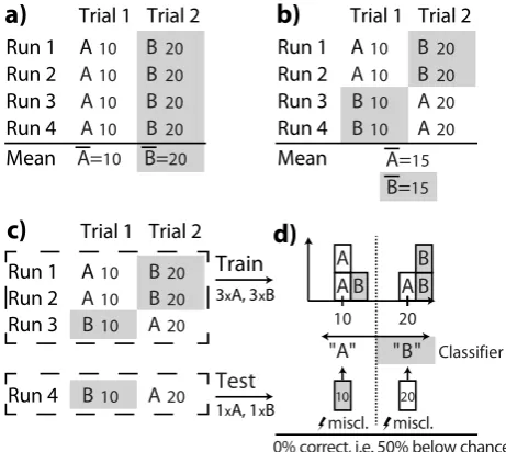
Figure 1. Example experiment. a,b) Experimental designs to test two experimental 

conditions A (no background) and B (grey background) in four runs. Small numbers  (10, 20) are example data for each experimental trial.  ,  denote condition specific  means. The design in panel a) cannot distinguish presentation order effects from ef‐ fects of the experimental conditions, because all first/second trials are also A/B trials.  The observed difference in means  10, 20  could thus arise from a difference  in either condition or trial number. In contrast, the design in panel b) controls the  confound “trial order” using counterbalancing. Even if data (small numbers) would  only depend on the trial number, as in this example, mean and variance of both ex‐ perimental conditions are equal ( 15), and thus standard statistics such as a t‐ test will not indicate a difference between the conditions: The confound control  worked. c,d) The same experimental design with leave‐one‐run‐out cross‐validated  classification. Panel c) shows partitioning of the data into training and test set for one  cross‐validation fold, and d) demonstrates that systematic misclassification of all test  data arises, resulting in 0% correct predictions. Systematic misclassification will also  occur in all other cross‐validation folds (not shown). Thus, the intended confound  control failed. Note that the reason for this systematic below‐chance accuracy is nei‐ ther an imbalanced number of training or test samples between conditions (nA = nB = 3  in each training set; nA = nB = 1 in each test set), nor is it specific to any particular clas‐

sifier, nor to cross‐validation in general. It is instead caused by a “design–analysis”  mismatch between a counterbalanced design and the cross‐validation scheme em‐ ployed in the analysis. 

 

Counterbalancing works as expected for the t‐test 

To test whether counterbalancing works as expected and indeed removes the  confounding effect of trial order, we can calculate what would happen if  there was no difference in the experimental conditions A and B, but the data  were only influenced by the confound “trial order” that is to be controlled.  Figure 1a and 1b show such a situation: Neuroimaging measurements are y =  10 in all first trials and y = 20 in all second trials. Whereas the experimental  design in Figure 1a does not allow to distinguish if an observed difference  between A and B arises from a true difference between the condition or be‐ cause A was always presented before B, the counterbalanced setup in Figure 

a)

Trial 1 Trial 2 Run 1 A10 B20 Run 2 A10 B20 Run 3 A10 B20 Run 4 A10 B20 Mean A=10 B=20

b)

Trial 1 Trial 2 A10 B20

A10 B20

B10 A20

B10 A20

Mean A=15

B=15

Run 1 Run 2 Run 3 Run 4

Run 1 A10 B20 Train

1xA, 1xB 3xA, 3xB

Run 2 A10 B20 Run 3 B10 A20

Run 4 B10 A20

c)

Trial 1 Trial 2

0% correct, i.e. 50% below chance

[image:6.595.180.411.72.278.2]

6

1b does allow this distinction. Collecting the counterbalanced measurements for each condition A and B across runs yields yA = [10 10 20 20] and yB = [20 20

10 10]. Clearly, a t-test would not indicate a significant difference between both conditions, because the data values are identical in both. Counterbalanc-ing therefore worked as intended: The factor “trial order” heavily confound-ed the data, but it had no systematic effect on the outcome of the statistical test.

Counterbalancing does not work for leave-one-run-out cross-validation

What happens if the counterbalanced but confounded data from Figure 1b is analysed with cross-validated classification instead of the t-test? Cross-validated classification is a standard MVPA method to estimate how well a classifier can learn from examples to predict (“decode”) the experimental condition of independent data, and can serve to test for statistical dependency between conditions and data like the t-test above (Haynes and Rees, 2005; Kriegeskorte et al., 2006; Norman et al., 2006). Although cross-validated clas-sification is typically applied to multivariate data, it can be applied to one-dimensional data equally well.1

In the same way as for the t-test above, we can check whether counterbalanc-ing the potential confound “trial order” will also prevent unexpected effects on the outcome of the cross-validated classification analysis by assessing its performance on the confounded but counterbalanced data from Figure 1b. Selecting a specific cross-validation scheme, i.e. how to separate data into training and test sets in the different folds, is one required analysis decision. The stratified leave-one-run-out cross-validation scheme in this example is common in neuroimaging because – in contrast to data from the same run – different imaging runs can be considered approximately statistically inde-pendent. Each run contains equally many samples per class, so the cross-validation is also balanced. Because the confound “trial order” has been con-trolled by counterbalancing and we know that there is no effect of the exper-imental condition, the classifier should not be able to distinguish between the classes. In a balanced setting with two classes, “cannot distinguish” translates to a classifier that assigns conditions to data in a non-systematic fashion, lead-ing to an expected classification performance around 50%.

1 _{Cross-validated classification is performed by repeatedly splitting the measured data samples}

Görgen et al., SAA

7

Instead, the obtained accuracy is 0% when performing the analysis, i.e. 50% below chance. This means that every single data sample was misclassified (Figure 1d). Despite the absence of a true effect, our result is worse than chance, demonstrating that in this example counterbalancing completely failed to control the confound “trial order”.

Standard control data analysis fails to detect the problem

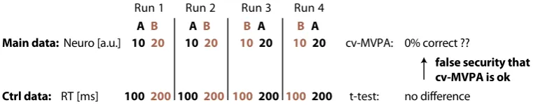
In an actual experiment, a researcher of course cannot know that no true ef-fect is present in the data. Since the result systematically deviates from chance, they might even suspect that a true effect is present, but they might not be sure how to interpret a systematic below-chance accuracy (cf. Allefeld et al., 2016; Kowalczyk, 2007). Because of this, they would probably conduct further analysis to look for the source of the unexpected behaviour. For example, the researcher might perform a control analysis on reaction times that were rec-orded together with the neural data. The idea is that a potentially confound-ing variable (attention level, task difficulty, etc.) will influence both the exper-imental and the control data. Consequently, finding an effect on the control data would demonstrate that the main results could alternatively be ex-plained by that confound. In this example, assume that the reaction times depend solely on trial order, just as for the neuroimaging data. For example, in first trials participants were more vigilant and responded faster, whereas in second trials their attention level was decreased and they responded more slowly (Figure 2).

8   

 

 

Figure 2. Mismatch between main analysis and control analysis. A standard control 

analysis fails to detect the problem from the initial example. Upper panel: Leave‐one‐ run‐out cross‐validated decoding applied to counterbalanced data without a true  experimental effect but with a “trial order” confound leads to a puzzling classifica‐ tion accuracy of 0% (Figure 1b‐d). Lower panel: A t‐test applied to reaction times as  control data does not find a difference and thereby fails to detect the problem gener‐ ated by the mismatch between the counterbalanced design and the cross‐validated  analysis. This may lead to a false sense of certainty that results from the main analysis  were not explained by a confound. 

 

Problem summary 

This initial example illustrates two of our main points. First, the design prin‐ ciple (counterbalancing) used in the experimental design comes from the es‐ tablished corpus but was paired with an analysis method (cross‐validated  classification) which does not. What the researcher overlooked here was that  design principles and analysis methods do not stand on their own but work  in tandem, and using another analysis method led to a “design–analysis  mismatch”. Second, using a standard control data analysis to diagnose the  problem failed, because it did not use the same analysis method, producing a  mismatch between main analysis and control analysis. Many problems that  arise with the use of novel analysis methods are caused by these or similar  kinds of mismatch: between design and analysis, different analysis steps, dif‐ ferent design principles, or analysis and statistical assumptions (see below).  Note that the focus of this paper is not the specific problem outlined above,  for which we could provide an explanation and solution at this point; nor is it  to provide an exhaustive overview of possible errors. Instead, we introduce a  general approach to diagnose problems, in form of a principled form of con‐ trol analysis for any number of errors. 

We now introduce this control analysis and demonstrate it on the problem of  the initial example. After that, we explain the origin of problem, provide two 

solutions, and discuss generalisations (sections “SAA as a guide to solve the  problem of the initial example” and following). We especially point out what  property renders the t‐test valid but cross‐validated decoding invalid and  that employing SAA to potential solutions can help to test if they work as  expected. 

Note that the confounding effect that we demonstrate in this example is not a  purely theoretical construct. It is also not simply remedied by increasing the  number of subjects or the number of runs per subject; only substantially in‐ creasing the number of data points per run would help. We demonstrate this 

A B A B B A B A

Run 2

Run 1 Run 3 Run 4

100 200 100 200 100 200 100 200

RT [ms] t-test: no difference

Neuro [a.u.] cv-MVPA: 0% correct ??

false security that cv-MVPA is ok

10 20 1020 10 20 10 20

Main data:

[image:9.595.107.488.71.146.2]

Görgen et al., SAA

9

on real empirical data with multiple subjects in the supplement (SI2). A nor-mal-sized empirical data set is also used in our second demonstration of an-other confounding effect below.

The Same Analysis Approach

Problems like those in the initial example are hard to detect, because seem-ingly the experiment was designed correctly by using counterbalancing to neutralize a common confound. While an in-depth examination of design, analysis, and statistics might have alerted the researcher to the problem, it is often hard to determine what exactly to look for, especially for novel analysis methods with little practical experience. Performing empirical control anal-yses is a good idea, but can systematically fail if analysis methods differ be-tween main and control analyses, as we demonstrated above.

In addition to theoretical examination and standard control analyses, we pro-pose to perform the following types of analysis:

Type 1) Apply the same analysis method used for experimental data to variables of the experimental design. Perform positive and negative control analyses on

syn-thetic noise-free data sets, each created from single variables of the experi-mental design, and analyse them with the main analysis method. Positive control analyses (see e.g. Fedoroff and Richardson, 2001) test if design varia-bles that should influence the experimental outcome – typically the experi-mental variable – indeed yield significant results; failing these tests demon-strates that the experimental setup (design, analysis method, or their combi-nation) are not suitable to detect the effect of interest. In more complex de-signs these should also test latent design variables that describe dependencies within the design. Negative control analyses test if design variables that

should not influence the experimental outcome indeed do not yield significant

results; failing these tests indicate that the variable is a potential confound, and/or that confound control did not work.

Type 2) Apply the same analysis method used for experimental data to empirical con-trol data. The main analysis method is applied to additionally measured

vari-ables (e.g. reaction times, age, IQ). Since control data provide a proxy for the main results, here a result indicates how the main analysis would respond if the actual data were influenced by a confound.

Type 3) Apply the same analysis method used for experimental data to synthetic null data. Applying the same analysis to multiple realisations of synthetic null

data tests if the false positive rate (the alpha level) is indeed as expected, and provides other general information on the null distribution of to be expected outcomes, such as range and shape.

efficient-10

ly detect, avoid, and eliminate confounds, not to create unnecessary workload for experimenters.

SAA to detect the problem of the initial example

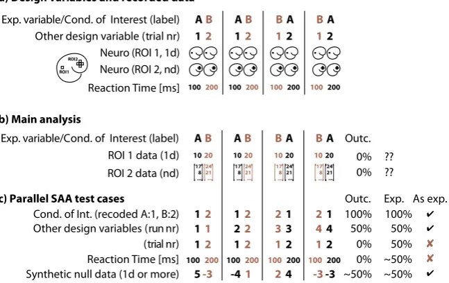
To illustrate SAA, we return to the initial example: An experiment with four runs and two trials per run, one for each experimental condition A and B, with presentation order counterbalanced across runs. Neurophysiological data is measured from a single voxel (ROI 1) and a larger region of interest (ROI 2). Additionally, reaction times are measured (Figure 3a). As assumed above, the neurophysiological example data are not influenced by the exper-imental condition, but only by the confounding factor “presentation order". In applying leave-one-run-out cross-validated classification we find 0% accu-racy in both ROIs in the main analysis, leaving us with the question how to interpret this result (Figure 3b).

We now use SAA type 1 (Figure 3c): the same analysis on design variables. This experiment has the three design variables “experimental condition” (positive control), “run number” and “trial number” (both negative controls). The experimental condition can be translated into pseudo-data by using the assignment A = 1 and B = 2. The analysis result of 100% accuracy confirms that cross-validated classification could detect an effect of the experimental manipulation if there was one (“positive control analysis”). Run number (1–4) and trial number (1 or 2) can be directly used as pseudo-data. Here the sis on run number results in the expected chance level of 50%, but the analy-sis on trial number results in 0% correct, providing a strong indication that a “trial order” confound could explain the observed below-chance accuracy (failed “negative control analysis”). Apparently, cross-validated classification is susceptible to this confound even though counterbalancing has been em-ployed to counteract it.

Following SAA type 2, we next apply the same analysis to the reaction times as control data, and find again an accuracy of 0%. This provides evidence that the “trial order” confound indeed influences the data.

Görgen et al., SAA 

11   

 

Figure 3. The Same Analysis Approach (SAA) applied to the initial example. a) De‐

sign variables of initial example (experimental conditions/trial number) and assumed  data (neural data from a one‐dimensional and another high‐dimensional ROI, reac‐ tion times). b) Features of neural data used in the main analysis. One data point (ROI  1: one‐d, ROI 2: high‐d) is available per trial. c) Parallel SAA analysis on test data: one  data point is available per trial, either generated from design properties (condition of  interest, run nr, trial nr), control data (RT), or synthetic null data. Abbreviations in  figure: “Outc.”: Outcome; “Exp.”: Expected; “~50%”: 50% plus/minus statistical devi‐ ation. 

 

Had the experimental design contained additional variables, we could have  systematically gone through all design variables, each time used the design  variable instead of measured data, performed the same analysis on these val‐ ues, and checked if the influence of this variable is as expected. 

Note that, except for type 2, SAA does not rely on real data. Therefore, the  problem with this combination of experimental design and analysis method  could have actually been detected (and solved, see below) before data were  collected. 

SAA as a guide to solve the problem of the initial example 

The analyses above demonstrate that the presentation order confound lead to  below‐chance classification and thereby explains the result of the main analy‐ sis. Further theoretical examination based on these results along the lines of  Figure 1d reveals that the culprit is a mismatch between counterbalanced  design and cross‐validated analysis, in particular that the design factor “trial  order” is not counterbalanced within each training and test set. One element that  might be confusing in this context is the terminology: The analysis is actually  “balanced”  in  the  sense  in  which  the  term  is  normally  used  in  cross‐ validation, which is to say that the number of training samples per class are  equal in each partition. Having both “balanced” data (presentation order) as  well as a “balanced” cross‐validation scheme (number of sample per class) 

b) Main analysis

c) Parallel SAA test cases

ROI 2 data (nd) 178 ... 24 21 ... 17 8 ... 24 21 ... 17 8 ... 24 21 ... 17 8 ... 24 21 ... Exp. variable/Cond. of Interest (label) AB AB BA BA

50% (trial nr) 12 12 12 12 0% ✘

100200 100 200 100200 100200 ~50%

Reaction Time [ms] 0% ✘

0% 0%

?? ??

~50% Synthetic null data (1d or more) 5-3 -41 24 -3-3 _~50% ✔

12 12 21 21 _100% 100% ✔

Cond. of Int. (recoded A:1, B:2)

ROI 1 data (1d) 1020 1020 1020 1020

Exp. As exp. Outc.

Outc.

✔ 50% Other design variables (run nr) 11 22 33 44 50% a) Design variables and recorded data

12 12 12 12

Other design variable (trial nr)

100200 100200 100200 100200

Reaction Time [ms]

Exp. variable/Cond. of Interest (label) AB AB BA BA

ROI1

[image:12.595.137.461.78.282.2]

12

makes it difficult to detect that the cross-validation is both “balanced and “not balanced” at the same time.

Note that the origin of the problem in this specific example is indeed only the missing counterbalancing in each cross-validation fold, and neither the analy-sis type (t-test vs decoding) nor the dimensionality of the data (the demon-stration actually is one-dimensional). Cross-validated MANOVA (Allefeld and Haynes, 2014), cross-validated Mahalanobis distance (Diedrichsen et al., 2016) used in RSA (Kriegeskorte et al., 2008), or any other cross-validated distance measure will all suffer from the same problem and systematically estimate negative distances, which are as confusing as below-chance results.

Two potential solutions and SAA to verify whether they work

One possible remedy for this problem is not to use counterbalancing but ran-domization, i.e. to randomly decide for each run independently whether to use the trial order AB or BA. We can now employ SAA again to test if the

solu-tion indeed works as expected, by re-running the same analysis on the design

variable “trial number” for randomized designs. When simulating many ex-periments, we find that the average classification accuracy is indeed 50% (the chance level), i.e. that the confound is statistically controlled. Looking at the individual outcomes, however, we find that 50% accuracy itself never occurs; rather, 0% occurs in 3/8, 75% in 1/2, and 100% in 1/8 of all randomizations (supplemental Figure A). SAA thus revealed that randomization does not seem an ideal solution in this context.

Another possibility to solve the problem would be to keep the design, but to use a validation scheme which ensures that the confound is counterbalanced in each test set, i.e. that each contains equally many AB and BA runs. This can be achieved by leaving out two runs (training sets in the four folds: runs 1 & 2, runs 3 & 4, runs 1 & 4, runs 2 & 3; supplemental Figure B). We can again employ SAA to test if this new analysis solves the problem. This time the result is indeed 50% for every single experiment, and not just on average as above. These two possibilities are of course not exhaustive. Since in this example the problem is related to the way cross-validation is implemented, another alter-native would be to replace classification accuracy by a (multivariate) test sta-tistic that does not need cross-validation.

Please note that the example here has been deliberately chosen to be as small as possible. The demonstrated systematic negative bias will, however, also occur in larger, real datasets if trial order has an effect on the data and leave-one-run-out cross-validation is used. The negative bias may not be as extreme as in the example, but can easily be large enough to suppress real effects and/or lead to confusing significant below-chance accuracies. See supple-mental section SI 2 for a demonstration on a real empirical dataset.

Related work and generalisation (initial example)

Görgen et al., SAA

13

majority classifier (that simply predicts for each test data the label that is most common in the training set ignoring any properties of the data) will yield 0% when leave-one-out cross-validation is employed on a balanced data set (with equally many samples per class). While the example is simpler than ours and critically depends on different numbers of exemplars per class, it already has the same general structure as ours, because again balancing is ignored when splitting data into training and test sets. The second example is “anti-learning” (Kowalczyk, 2007), which demonstrates that datasets with specific properties will always yield below-chance accuracies for a large number of classifiers, independent of any specific design property or validation scheme. The third cause hinges on using the binomial test for single cross-validated accuracy estimates, which will yield too many significant below-chance re-sults (Jamalabadi et al., 2016; Görgen et al., 2014) and above chance rere-sults (Noirhomme et al., 2014; Görgen et al., 2014). Another scenario in which counterbalancing also unexpectedly fails to control a confounding factor in MVPA has been described by Todd et al. (2013). It differs from our example because in theirs individual decoding analyses are calculated for each unit (subjects in their example, runs in ours), whereas only a single decoding analysis using all units is calculated in our example. Other major differences are that it causes above chance results, not below chance results, and that it does not depend on any particular cross-validation scheme, which is the crux in our example.

Our example demonstrates that systematic below-chance classification accu-racies can be caused by a design–analysis mismatch, which can even occur when employing only basic experimental methodology. In the specific exam-ple above, the design variable “trial order” was controlled. The problem, however, is not specific to controlling time or sequence effects; the same logic applies to counterbalancing any other variable against the experimental vari-able. In general, it often has unexpected consequences if design features which are implemented with respect to the full data set are ignored when data is split into training and test sets for cross-validation. Examples for this are cases where each class has an equal number of samples in the full data set but differing numbers in each training and test set, or cases of “dissolving strata” such as the assignment of patients and their matched controls to dif-ferent partitions.

Principles for setting up SAA

14

Test data

Design variables: These can be explicit design variables such as the

experi-mental condition or the level of a factor in a factorial design, or implicit de-sign variables such as the sequential number of the trial within run or the repetition number of a stimulus.

Control data: These are additionally recorded data such as reaction times, error

rates, motion correction parameters, eye-tracking data etc. Possible across-subject data include age, gender, IQ, or personality scores.

Simulated data: Simulations open a wide range of possibilities. Data may be

generated so that there is no effect (null data) or there is a specific effect, that a confound is present or not present, or combinations thereof. They may be simplistic, for example data consisting of only 1s (constant data), or they may come from a generative model attempting to capture as many aspects of real data as possible (distribution, autocorrelation across time and space, hemo-dynamic response, effect size, variation across measurements, trials, runs, and subjects). A special case are modified data from the same experiment, e.g. shifted by one trial (Soon et al., 2014), or experimental data unrelated to the experiment, such as resting-state data (Eklund et al., 2016).

Mapping function: In some cases, test data may be in a form that cannot be

processed by the “same analysis”. An example is the experimental condition, which is a nominal label and therefore not compatible with a classifier that expects numerical input. Such categorical data may be mapped to input data in several ways: Conditions are arbitrarily assigned numerical values (see example above), or encoded as multiple dummy variables (1 if a trial belongs to a condition, 0 otherwise), or assigned to randomly chosen multivariate patterns. Another case are analyses that use intrinsically multivariate measures such as pattern correlation or cosine distance, e.g. in representa-tional similarity analyses (RSA; Kriegeskorte et al., 2008). Here, simple math-ematical or statistical models can be used to create multivariate data, where similarities are determined by the input variable. Indeed, there is high value in creating different test cases that all map the same variable to test data, but with different mapping functions, to understand how the analysis pipeline reacts to input that might be encoded different than expected (e.g. if it is not clear which coding scheme the brain employs to encode a specific stimulus). Depending on the complexity of the mapping function, there is a continuum between SAA on a simple design variable and a full-blown simulation.

Test range

Görgen et al., SAA

15

Test case

Together, each combination of test data, mapping function, test range, and outcome specifies a unique test case.

Expected outcome

Whenever possible, each test case should come with a defined expectation (e.g. chance level classification if there is no effect), and interpretations if the expectation is fulfilled or violated. Depending on the test data (see below), an expectation may be a specific value (e.g. an accuracy of 50%) or a distribu-tional property (e.g. average accuracy 50%).

Deterministic vs stochastic tests

When the test data are fixed, e.g. noise-free pseudo-data generated by a de-terministic mapping from a design variable, there is only one corresponding analysis result, and the interpretation of the result depends on this single fixed value. For noisy data like experimental control data the outcome is still fixed, but its interpretation is not straightforward and a statistical test may be necessary to determine whether the result is significant. In a simulation in-corporating random variation, the simulation has to be run a sufficient num-ber of times to assess properties of the distribution of outcome values, e.g. mean, variance, or number of significant outcomes. For the latter, statistical testing and simulations can be combined by looking e.g. at the frequency with which the statistical test indicates a significant result across simulation runs, to determine whether the test is valid under the given circumstances.

Recommendations when using many statistical tests

It is simple to implement a large number of SAA tests, especially using simu-lated data. If the results are assessed by a statistical test, the number of false positives will increase with the number of tests, so that the significance level has to be adjusted. This raises the question how to balance between sensitivi-ty and specificisensitivi-ty for possible confounds, and how to efficiently detect prob-lems within many test outcomes. For this purpose, we suggest the following measures:

Adjusting the significance level only for less important tests. Tests should be

sepa-rated into a small number of important tests, which are targeted at potential confounds that are expected to exert a strong influence, and a possibly large number of less important tests that are only performed to be on the safe side. For the first class, sensitivity (as controlled by the significance level) is kept high, while the second class is corrected for multiple comparisons.

A priori checks vs problem diagnosis. When SAA is set up prior to data collection

(see below) or when no signs of a problem exist in the analysis of experi-mental data, the sensitivity can be lower than when trying to find the source of a concrete problem which is evident in main analysis.

Sorting test cases by influence. Tests should be sorted according to whether a

16

an unexpected result, it is likely that there is a very deep-seated and general problem which also influences the outcomes of other, more specific tests.

Interpretation of results. Problem diagnosis should not rest simply on whether

a statistical test gives a significant result, but the researcher should use their judgement to decide whether a confound is likely to be relevant in the main analysis. More realistic simulations can help to assess the practical impact of a confound.

Correlating SAA outcomes and main outcomes as additional check or to detect location-specificity

If multiple SAA test cases indicate potential confounds, only some of them may actually affect the main analysis. To check this, correlations can be calcu-lated between the outcomes of one or multiple SAA test cases and the out-comes of the main analysis. As with any statistical test, a negative result does not mean that the tested variable is not a potential confound, but a positive result strongly indicates that it is (see Reverberi et al., 2012 for an application example). Moreover, if the same main analysis is performed on different segments of the data, e.g. brain regions or time points, correlations to SAA outcomes can be calculated for each segment to detect location-specific con-founding effects, e.g. a confound may only affect motor cortex but not visual cortex.

When to use SAA

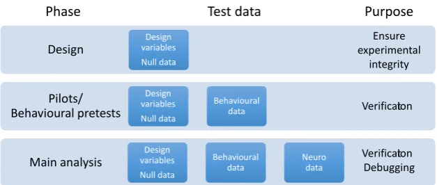
SAA helps to find solutions when experimental data have already been ac-quired and their analysis indicates that there may be a problem; in some cas-es, however, it may come too late at this phase. We therefore recommend to use SAA systematically during different phases of a study (Figure 4):

Design phase. Tests can already be set up when designing and implementing

an experiment to ensure that the analysis pipeline works as expected and that the design matches the analysis.

Piloting phase. During behavioural pre-tests or pilot studies tests can be used

to check whether potential confounds are present in participants’ responses.

Main analysis phase. After data collection, tests can be run on control data to

Görgen et al., SAA

[image:18.595.141.455.69.202.2]

17

Figure 4. Guideline for using SAA in different phases of a study.

Empirical Example: Variance confound in classification

In this section, we demonstrate how to use SAA to diagnose a problem on real empirical data. A researcher performs an experiment where participants press a button with either the left or right index finger in response to visual stimuli. Left button presses are more frequent than right button presses, 12 vs 3 trials per run (following e.g. an oddball paradigm, Squires et al., 1975). BOLD data are recorded in 6 runs from 17 participants. To identify brain re-gions that carry information about which button was pressed, the researcher applies leave-one-run-out cross-validated classification to parameter esti-mates from voxels within a searchlight, using a linear support vector ma-chine. For a time-resolved analysis, they use finite impulse response (FIR) regressors comprising 16 two-second time bins (cf. Kriegeskorte et al., 2006; Soon et al., 2008). Because they are aware that imbalanced data pose a prob-lem for many classification algorithms (He and Garcia, 2009), they use a sin-gle set of regressors for modelling left and right button presses, respectively (Allefeld and Haynes, 2014; Haxby et al., 2011; Norman et al., 2006). For each FIR time bin, this yields a single parameter estimate image per condition and run, all of which are then used for time-resolved searchlight classification. Subject-wise classification accuracy maps are then entered into a second-level

t-test across subjects against the chance level of 50%.2

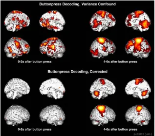
There are clear expectations for the result of this analysis. First, information should be localized mainly in motor regions because the analysis contrasts two different movement conditions. Second, above-chance classification should be possible no earlier than 4s after button press because of the hemo-dynamic delay. The results, however, show significant information in large regions across the entire brain, and already at 0-2s after button press (Figure 5, top). Apparently, something in the analysis went wrong.

2 _{This example was constructed using data from an unpublished study on rule representation.}

Preprocessing, parameter estimation, and second-level analysis of fMRI data were performed with SPM8 (Wellcome Department of Imaging Neuroscience) and searchlight classification with The Decoding Toolbox (Hebart et al., 2015) using LIBSVM (Chang and Lin, 2011).

Main analysis Pilots/ Behavioural pretests Design Design variables Null data Design variables Null data Behavioural data Design variables Null data Behavioural data Neuro data Ensure experimental integrity Verification Debugging Verification

18

Figure 5. Results of confounded and corrected example fMRI analyses. Top:

Signifi-cant results of button press classification with variance confound on real data 0–2s and 4–6s after button press. Run-wise GLM parameter estimates were calculated us-ing 12 trials for left and 3 trials for right button presses. Bottom: Same as above, but using 12 left and 12 right button presses to calculate run-wise estimates. – All dis-played voxels show significant effects at p ≤ 0.001 uncorrected. All larger clusters are also significant at p ≤ 0.05 FWEc-corrected; only in the corrected analysis at 0-2s no cluster survives FWEc correction (bottom left). Supplement Figures D (SI 5) contain more combinations & time bins.

SAA setup

The researcher wants to use SAA to diagnose the suspected problem, check-ing for temporal, attention, and sequence effects, as well as details of the task. They create test cases by making the following decisions:

Test data:

Synthetic noise-free positive test

– The condition of interest itself (“side”)

Empirical negative tests

– Attention effects: response time, correctness of response

Synthetic noise-free negative tests

– Temporal effects: number of trials (“ntrial”), time of button press, target onset

– Sequence effects: value of all these variables from the previous trial (“t-1”)

[image:19.595.139.457.71.350.2]

Görgen et al., SAA 

19   

Synthetic null‐distribution negative tests 

– 10,000 one‐dimensional random null datasets (“randn1”, “randn2”, etc.)  drawn from the standard normal distribution) 

Numerical test data (e.g. time, number of button presses) are used as input  values for the analysis as‐is (e.g. the values 1, 2, …, for trial numbers). Cate‐ gorical data (side of button press) are mapped to dummy variables (here a  two‐dimensional vector, that is [1 0] for trials that expect a left button press,  and [0 1] for trials that expect a right button press). 

Test range: Test data are generated on the level of single‐trial values, and the  whole analysis from there to the second‐level t‐test on accuracies is consid‐ ered. The analysis steps in this range are: 1) computing run‐wise parameter  estimates, 2) leave‐one‐run‐out cross‐validated classification, and 3) a group  level t‐test applied to subject‐wise classification accuracies. Outcomes are  subject‐wise accuracies (visualized through box plots), p‐values of the second  level t‐test, and the frequency with which the test indicates significance for  null data. 

To increase the sensitivity of SAA, the researcher sorts the test cases into dif‐ ferent categories, labelled “sanity checks”, “design random” (test cases for  which the result can vary for different test cases), and “control data” (Figure  6). Supplement section SI 6 provides a more detailed explanation including  the concrete steps to setup this SAA analysis. 

 

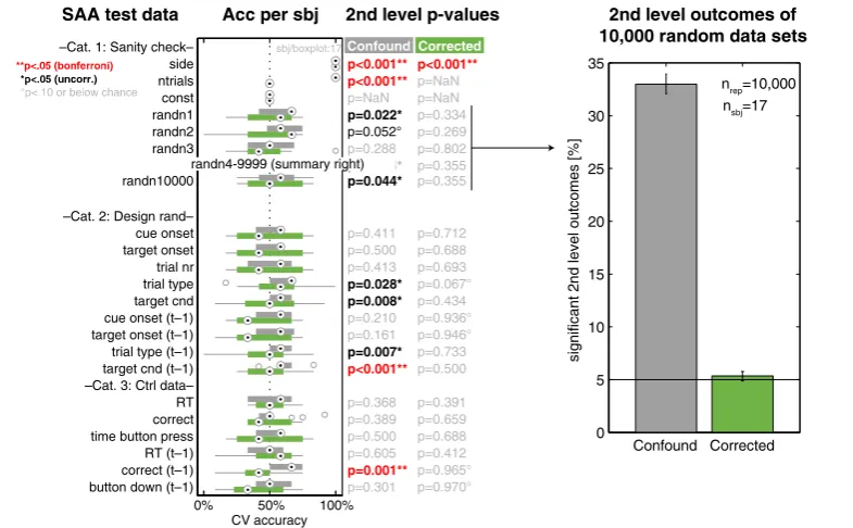
Figure 6. SAA results for different test data. Left panel: Distribution of accuracies per 

subjects as box plots with medians (filled circles) and outliers (empty circles) before  (grey) and after correction (green). Small dotted line marks the chance level of 50%.  “2nd _{level p‐values” column provides the p‐values for a one‐sided t‐test across sub‐}

jects against 50%. Right panel: Summary for the 10,000 simulated random null data  sets (“randn1” – “randn10000”), showing the relative frequency of cases where the  SAA result was significant (p ≤ 0.05). 

Confound Corrected 0 5 10 15 20 25 30 35 si gni

ficant 2nd l

evel

outcom

es [%

]

n_rep=10,000 n_sbj=17

Corrected

CV accuracy50%

0% 100% p<0.001** p=NaN p=NaN p=0.334 p=0.269 p=0.802 p=0.355 p=0.355 p=0.712 p=0.688 p=0.693 p=0.067° p=0.434 p=0.936° p=0.946° p=0.733 p=0.500 p=0.391 p=0.659 p=0.688 p=0.412 p=0.965° p=0.970° Confound

–Cat. 1: Sanity check– side ntrials const randn1 randn2 randn3

–Cat. 2: Design rand– cue onset target onset trial nr trial type target cnd cue onset (t–1) target onset (t–1) trial type (t–1) target cnd (t–1) –Cat. 3: Ctrl data– RT correct time button press RT (t–1) correct (t–1) button down (t–1) randn10000 p<0.001** p<0.001** p=NaN p=0.022* p=0.052° p=0.288 p=0.044* p=0.044* p=0.411 p=0.500 p=0.413 p=0.028* p=0.008* p=0.210 p=0.161 p=0.007* p<0.001** p=0.368 p=0.389 p=0.500 p=0.605 p=0.001** p=0.301

randn4-9999 (summary right)

SAA test data Acc per sbj 2nd level p-values 2nd level outcomes of 10,000 random data sets

[image:20.595.112.505.413.656.2]

20

Interpretation of SAA results

The results shown in Figure 6 show significant effects for several negative control analyses, for which no effect was expected.

Focusing on the “sanity check” category first, the researcher is reassured by the outcome of the positive control analysis “side”, which confirms that the analysis is able to distinguish left and right button presses if there is a differ-ence between the corresponding trials. There is also a significant effect for “ntrial”, the number of trials per condition, which is not surprising since there is a systematic difference between conditions in the number of trials (3 vs 12). By contrast, there is an unexpectedly high number of significant re-sults for random null data: the second-level t-test rejected the null hypothesis in 33% (CI95%=[32.1%, 33.9%]) of the 10,000 instances (at α = 0.05) instead of the expected 5%.

The SAA has therefore confirmed the suspicion that there is a problem. The increased false positive rate of the null simulations strongly suggests that it has to be a more general aspect of the design or some property of the analysis procedure, because neither the experimental variable nor any other design factor had any influence on the simulated null data. A peculiar property of the design is the different number of trials in the two conditions. The re-searcher assumed to have dealt with this by applying classification not to single-trial data but to run-wise parameter estimates – but what if this was not enough?

The researcher checks this hypothesis by modifying the SAA analysis so that equally many trials are used to calculate the estimates for left and right but-ton presses in each run. Indeed, after this correction (green elements in Figure 6), the number of “significant” results in the 10,000 instances of null data drops to 5.4% (CI95%=[4.9%, 5.8%]), consistent with a false positive rate of 0.05. The only test case that remains significant is the positive control using the variable of interest itself (“side”), which is how it should be.

The result of the corrected analysis on the fMRI data (Figure 5, bottom) con-firms that the apparent confound has been removed; there is no significant effect present in the 0–2s time bin, and effects in the 4–6s time bin are located in motor and sensory regions as expected. Supplemental Figures D.1-D.8 in supplement section SI 5 show the time-resolved results for all combinations of 3, 6, and 12 button presses from each side, illustrating that problem is in-deed caused by the imbalance between trials and not by e.g. differences in power; choosing the same number of left and right trials always solves the problem.

Cause of the problem: Variance-based linear classification

Görgen et al., SAA 

21   

During experimental setup, the reasoning of the researcher was the following:  1) Classifiers are known to be sensitive to imbalanced training data, therefore  classification is applied to run‐wise parameter estimates, which are essential‐ ly averages across trials. 2) Linear classifiers are sensitive to linear differences  between class‐specific data distributions, i.e. differences in the class means.  3) If there is no effect, trial‐wise data from both classes comes from the same  distribution, and averaging over more or fewer trials does not change the  mean. 

The mistake in this argument is that while the difference in number of trials  per condition does not change the mean, it does change the variance of run‐ wise estimates. And contrary to common assumption (Kamitani and Tong,  2005; Naselaris et al., 2011; Norman et al., 2006), linear classifiers can not only  use differences in mean, but also differences in variance to achieve above‐ chance classification (Figure 7). This behaviour is not limited to specific types  of linear classifiers; it applies even to classifiers utilizing the means (cen‐ troids) of the data, such as nearest centroid classifiers or linear discriminant  analysis (explanation in caption of Figure 7, especially panels c,d). More gen‐ erally, linear classification based on the variance of parameter estimates can  come about by differences in the estimability of regressors (Hebart and Baker,  this issue). 

Note that successful linear classification that is based on differences in vari‐ ance is not a confound, because the classifier reveals a difference that truth‐ fully exists in the data (see also Davis et al., 2014 for other effects of variability  in MVPA). It can, however, be an interpretation error if this is interpreted as  showing a linear (mean) difference between conditions. In contrast, the em‐ pirical example contains a true confound, because the data from both classes  do not come from different distributions, but the variance difference between  both is induced during the analysis (Figure 7a,b). A detailed simulation for  SVMs and nearest centroid classifiers can be found in the supplemental sec‐ tion SI 7 (Figures E.1 and E.2). 

 

 

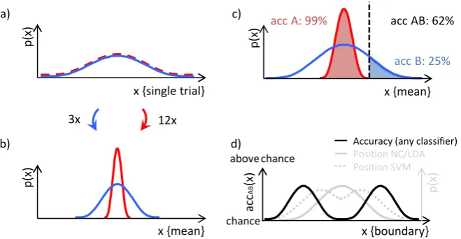
Figure 7. Induction of variance difference by design and successful variance classifi‐

cation with a linear classifier. a) Original probability distribution (one‐dimensional)  of single trial values for two classes (blue, red). b) Averaging (or regressing) different 

p( x) p( x) x {mean} p( x) x {single trial} 3x 12x x {boundary} chance a) c) ac c AB (x) above chance p( x) b) d)

acc A: 99%

x {mean}

acc B: 25%

acc AB: 62%

Accuracy (any classifier)

[image:22.595.134.464.547.718.2]

22

numbers of trials creates distributions that have the same mean but different vari-ance. c) Example of a linear classifier (classification boundary: black dashed line) that classifies between both classes above chance using the nonlinear variance difference between the two. d) Expected accuracy for classifiers with a decision boundary at different positions (black line), and probability distribution where a nearest centroid classifier or linear discriminant analysis (NC/LDA; grey solid line) or an SVM (grey dashed line) place the boundaries. The expected accuracy (black line) will at mini-mum be at chance level (when placed exactly at the common mean of both distribu-tions, or at plus or minus infinity) and otherwise above chance. Because the position of the boundary varies (grey lines), the expected accuracy for classifying between classes that differ in the nonlinear mean using a linear classifier is above chance. Note that successful linear classification between data classes that only differ in variance (panels c,d) is not a confound, because the classifier truthfully reveals a difference that exists in the data. It can however be an interpretation error if this is interpreted as showing a linear (mean) difference. In contrast, the confound in the example arises because the variance between both classes is induced during the analysis (panels a,b). Detailed simulations can be found in supplemental section SI 7.

Related work and generalisation (empirical example)

The main aim of this example was to demonstrate how SAA can be employed in practice. However, the example is also interesting in itself. Averaging be-fore classification and feature extraction from multiple trials bebe-fore more complex data analyses methods are standard analysis procedures. We advise to test for potential confounding effects through null simulations here. An-other important point relates to the inference from classification analyses: Since linear classifiers can successfully extract nonlinear information, success-ful linear classification does not allow direct inference on the linear versus nonlinear nature of representations (e.g. Kamitani and Tong, 2005; Norman et al., 2006; Naselaris et al., 2011; Diedrichsen and Kriegeskorte, 2017; Friston, 2009).

The example also demonstrates that confounds can arise through a combina-tion of analysis steps that pose no problems individually. These can be de-tected by simple simulations on synthetic null data if the same analysis is employed.

Discussion

intui-Görgen et al., SAA

23

tions but to explicitly check them, by applying the same analysis used for ex-perimental data also to design variables, control data, and simulated data. We now discuss a number of points that may need further clarification.

Keep it simple. A main focus of this paper is to introduce design principles to

create efficient control tests. We made a number of suggestions in this paper how this can be achieved. One main suggestion is “keep it simple”; other suggestions are to perform positive and negative control analyses on many simple control datasets that are each influenced by only one synthetic or em-pirical variable, and to create “time-shifted” datasets by using variable values from the previous trial to detect sequence effects which are common con-founds in neuroimaging. Further recommendations to keep SAA effective include adaptive alarm rate thresholds and correlating SAA to main analysis outcomes. However, we do not believe that these are the ultimate and only principles to set up efficient tests, nor that they fit all experimental para-digms. We rather conceive them as first suggestions, and hope that further principles for efficient tests will emerge from employing SAA in practice.

When to employ SAA. SAA can be used to diagnose problems that have

al-ready become apparent, but we recommend to use it continuously through all phases of a study – planning, piloting, and final analysis – to become aware of possible problems as early as possible. Side benefits of this practice are that it encourages to consider details of the analysis already at the design phase and therefore to tailor the design to the questions one wants to ask; that it can be used for power analysis (if sufficiently realistic simulations are implemented); and that it helps to detect simple programming errors (both in design and analysis, because SAA tests depend on both). Indeed, the sole process of set-ting up SAA at the design phase can prevent programming errors in the first place, because the coding scheme of variable names and content are fresh in mind when programming design and analysis at the same time, reducing the risk of confusion between both. In contrast, if time passes between setting up design and analysis, e.g. when data is recorded, chances to confuse variable names or coding schemes are much higher. SAA might also facilitate design optimization, but we believe that further investigation of potential negative side effects is necessary.

About our examples. In addition to describing and detailing SAA in general,

we illustrated it in two concrete examples. Their main function in this paper is to spell out in detail how SAA can be applied and how it uncovers poten-tial problems with a given data set or design.

However, both of them are also relevant on their own, because they reveal two relevant problems in MVPA: The initial example demonstrates that the classic strategy of counterbalancing the experimental design (leading to what is also known as a crossover designs) to control a confound can become inef-fectual if combined with an analysis method that uses cross-validation3_{. The}

3 _{In the specific example, the design variable “trial order” was controlled, but the same logic}

24

empirical example shows that differences only in variances yield successful linear classification, specifically demonstrating that inferring linear differ-ences from linear classification would be invalid (see “Cause of the problem: Variance-based linear classification”). In addition, we demonstrate that anal-yses of control data can fail, even if to-be-controlled effects are present, when different methods are employed for control and experimental analyses. The fact that neither example depends on the dimensionality of the data (both work for multi- and univariate data) demonstrates that unexpected con-founds are also not specifically bound to multivariate analysis, but can occur for univariate analyses as well.

Relevance. The fact that SAA would detect our examples as well as examples

from the recent literature, both MVPA specific (Todd et al., 2013; Woolgar et al., 2014; Noirhomme et al., 2014; Görgen et al., 2014; Jamalabadi et al., 2016) and more general (Kriegeskorte et al., 2009; Vul et al., 2009; Mumford et al., 2015), demonstrates the potential of SAA in aiding to detect easy-to-overlook problems. We have found it helpful in personal work, and are looking for-ward to seeing whether or not that will be the case in general. Finally, we see employing the same analysis method as especially important for control analyses, at least in addition to other analysis methods, because – as demon-strated – they can fail their purposes when different analysis methods are employed.

Not too few data; more data no remedy.4 _{A common misconception is that}

confounding effects occur only for small data sets, and that more data would reduce those confounds. While more data can help reducing effects of non-systematic confounds, simply adding more data is no universal solution, spe-cifically when confounding effects are systematically induced by design, such as in the examples that we demonstrate here. Indeed, the empirical example already has a normal-sized sample, and because the confounding effect is present in each subject, more subjects would even increase the effect strength. The same holds for the initial example if the presented design would be used for multiple subjects and a test would be applied on the group level (see sup-plemental section SI2). It would also stay a potential confound if the number of runs is increased. In the idealized case with no noise and no effect (as in the example), the classification accuracy would stay at 0% correct. In real data, for increasing number of runs the importance of the confound depends more and more on the relative effect sizes of confound and experimental effect. If no experimental effect is present, the primary effect measure (classification accu-racy) will come closer to chance level, but because the null distribution be-comes narrower, the confounding effect could still have a significant impact.

Differences between SAA and simulation studies. SAA shares aspects with

standard simulation studies that are routinely used to demonstrate merits and pitfalls of particular design or analysis methods. Like SAA, simulation studies demonstrate their claims through computation.

Görgen et al., SAA

25

SAA however differs from simulation studies in important aspects. First, it avoids a particular problem in simulation studies, which is to choose which settings are important to demonstrate generality. Because SAA is used for a

particular experiment, most parameters (such as number of subjects, etc.) are

fixed. Second, simulation studies typically include complex realistic simula-tions, to demonstrate the operation of a method in realistic scenarios. In con-trast, SAA is employed to perform sanity checks, which we believe can be effectively done with simple simulations. Whether or not this is the case, and which additional principles can help to create useful control analyses is an open question, that we believe will need to employ SAA in practice. Thus, SAA is not a theoretical tool to demonstrate a claim; it is an empirical tool to help creating better designs and analyses.

SAA and unit testing. SAA has been inspired by the practice of “unit testing”

in software development (Myers et al., 2011), i.e. writing software in the form of modules that each can be tested independently (for internal function) and in combination (for adherence to interfaces between modules). The situation in software development is insofar similar to that in neuroimaging that in principle the validity of an algorithm may be strictly proven, but the multi-tude of newly produced code makes that practically impossible. In contrast to unit-testing, SAA however does not test software modules, e.g. functions of an analysis package, but instead design–analysis combinations of specific experiments.

SAA in other fields. SAA shares its rationale with a number of other

scien-tific approaches. It follows the same logic as the routine use of positive and negative controls in disciplines like chemistry or molecular/cell biology (Fe-doroff and Richardson, 2001; Johnson and Besselsen, 2002), where the work-ing of the full analysis pipeline is tested for every experimental data again by analysing positive and negative probes alongside with the experimental data, e.g. during PCR, or in medicine, e.g. using diluent and histamine as controls in skin prick testing during allergy diagnosis (Rusznak and Davies, 1998).

Not a general solution. We would like to point out that although SAA is a

tool that can be generally applied to data analysis pipelines and is not special-ized to find specific kinds of problems in specific kinds of analyses, there is no guarantee that it will help to detect any kind of problem in any kind of analysis. Moreover, SAA in itself does not solve any problem, but merely points the researcher to possible problems that then have to be resolved on a case-by-case basis.

Conclusion. We hope that new developments in neuroimaging data analysis