A Study of mutispectral temporal scene normalization using pseudo-invariant features, applied to Landsat TM imagery

RIT Scholar Works

Theses Thesis/Dissertation Collections

10-1-1985

A Study of mutispectral temporal scene

normalization using pseudo-invariant features,

applied to Landsat TM imagery

William Volchok

Follow this and additional works at:http://scholarworks.rit.edu/theses

This Thesis is brought to you for free and open access by the Thesis/Dissertation Collections at RIT Scholar Works. It has been accepted for inclusion in Theses by an authorized administrator of RIT Scholar Works. For more information, please [email protected].

Recommended Citation

APPLIED TO LANDSAT TM IMAGERY

by

William J. VolchoK

A thesis submitted in partial fulfillment of the requirements for the degree

of Master of Science in the Center for Imaging Science in the College of Graphic Arts and Photography of the Rochester Institute of Technology

October, 1985

Signature of the Author

Center for Imaging Science

Accepted by

Rochester, New York

CERTIFICATE OF APPROVAL

M.S. DEGREE THESIS

The M.S. Degree Thesis of William J. Volchok has been examined and approved

by the thesis committee as satisfactory for the thesis requirement for the

Master of Science degree

Dr. John R Schott, Thesis Advisor

Dr. Willem Brouwer

Mr. Peter Engeldrum

Date

I

ROCHESTER INSTITUTE OF TECHNOLOGY COLLEGE OF GRAPHIC ARTS AND PHOTOGRAPHY

Title of Thesis: A STUDY OF MULTISPECTRAL TEMPORAL SCENE NORMALIZATION USING PSEUDO-INVARIANT FEATURES. APPLIED TO LANDSAT TM IMAGERY

I.

be of commercial use or for profit.

Signature

USING LANDSAT TM IMAGERY

by

William J. Volchok

Submitted to the

Center for Imaging Science

in partial fulfillment of the requirements for the Master of Science degree

at the Rochester Institute of Technology

ABSTRACT

A new technique for performing temporal image' normalization using pseudo-invariant features was investigated. The technique was applied to the six reflected spectral band images of the Landsat TM sensors. The temporal normalization of pseudo-invariant features yielded linear normalizing functions for all bands. The errors in the normalization of pseudo-invariant features was determined to be on the order of three digital counts, which was estimated to be equivalent to reflectance errors on the order of one percent reflectance. Temporal normalization of all features in the Landsat scene shows great potential for both quantitative and qualitative temporal change detection.

The author wishes to extend the greatest appreciation to Dr. John R. Schott for his support and guidance, during and prior to the developement of this thesis. Dr. Schott's efforts within the image science programs, especially the developement of the Digital Imaging and Remote Sensing (DIRS) Lab, have made him a valuable asset to the students and RIT.

In addition, the author would like to thank the following people for their advice and assistance:

Joe Biegel of the DIRS lab for his continuous critiques concerning scientific and statistical methods;

Peter Engeldrum and Willem Brouwer, members of the Center for Image Science faculty, for their contributions as thesis advisers;

All members of the DIRS lab for their help and cooperation throughout the experimental portions of this study.

This thesis is dedicated to my parents,

Ethel and Herbert, whose unquestioning support,

both moral and financial, lead to

the completion of this MS degree.

LIST OF TABLES . . . .

LIs'r OF FIGURES . . . .

1. INTRODUCTION . . . .

1.1 Objectives . . . . 1.2 Historical Background . . . . 1.2.1 Classification and Segmentation ... . 1.2.2 Atmospheric Models and Correction ... . 1.2.3 Image Normalization . . . .

1.3 Theoretical Background . . . . 1.3.1 Pseudo-Invariant Features (PIF's) ... . 1.3.2 Variance in Landsat Data . . . . 1.3.3 Normalization Using PIF's . . . . 1.3.4 Transformation Derivation Tecr~iques ... .

2 • ~.ER. I MENTAL ••••••••••••••••••••••••••••••••••••...•

2.1 Image Selection . . . .

2.2 PIF Classification and Segmentation ... . 2.2.1 Classification Procedures . . . . 2.2.2 Segmentation Procedures . . . .

2.3 Normalizing Transformation Determination ... . 2.3.1 Transform Determination via Histogram

Specif ication . . . . 2.3.2 Transform Determination via Linear

Histogram Analysis . . . .

2.4 Transformation Analysis . . . . 2.4.1 Comparison of Transform Derivation

Techniques . . . . 2.4.2 Empirical Transformation Error Analysis .... . 2.4.3 Error Propagation of Transform Errors ... . 2.4.4 Estimation of Reflectance Errors ... . 2.4.5 Full Scene Transformation and

Temporal Changes . . . . 2.4.6 Secondary Scene Comparison . . . .

3.. RESULTS ... ..

3.1 Images Selected and PIF Segmentation ... . 3.2 Spectral Normalization Transforms ... .

3.3 Transformation Method Comparison ... .

3.4 Transformation Error Analysis ... .

3.5 Relative Reflectance Errors . . . .

3.6 Full Scene Normalization and Temporal Changes .. .

3.7 Normalization of Secondary Images ... . 4. CONCLUSIONS . . . .

5. RECOMMENDATIONS FOR FUTURE WORK ... .

REF'ER.ENCES ... ..

APPENDIX A Spectral Response Characteristics of the Landsat TM-4 and TM-5 Reflected Energy Sensors ...

APPENDIX B Derivation of Histogram Specification Techniques ... ..

APPENDIX C Derivation of Linear Histogram Analysis Operation (LHAO) . . . . APPENDIX D Summary of Image Storage and Computer

Program Algori thms . . . . APPENDIX E Error Propagation for Independent and

Correlated Errors ... ..

APPENDIX F Multiple Transform and Control

Po i n t Da ta ... ..

VITA ... ..

Table 1-1 Comparison of Landsat TM and MSS

Measurement Capabilities . . . . Table 1-2 Reflectance of Asphalt Pavement Samples ...

Table 1-3 Temporal Variation of Ratio Measurements ....

Table 2 1 TM Imagery Da ta . . . .

Table 2-2 PIF Classification Data . . . .

Table 2-3 PIF Sample Locations . . . . Table 3-1 Summary of Temporal PIF Image and

Transform Data . . . .

Table 3-2 RMS Errors Between Transform Methods ... . Table 3-3 RMS Errors Between Transformed Control

DC and Target Point DC . . . . Table 3-4 : Summary of Reflectance Conversion Data ... .

Table 3-5a : Summary of Normalized Sample DC

Signa ture Data . . . .

Table 3-5b Summary of Normalized Sample % Reflectance Signature Data . . . . Table 3-6 : Summary of Temporal PIF Image Data for

Rochester and Batavia Samples ... .

Table 3-7a : RMS Errors for Batavia Transforms:

Histogram Specified vs. LHAO Derived ... .

Table 3-7a RMS Errors for Normalizing Transforms:

Derived for Rochester vs. Batavia ... . Table F-l DC Values for Control Data . . . .

Table F-2 Multiple Transform Data, Slopes and

Intercepts . . . .

Figure 1-1

Figure 2-1

Figure 2-2 :

Figure 2-3a

Figure 2-3b

Figure 2-3c

Figure 2-3d

Figure 2-3e

Figure 2-4

Figure 2-5

Figure 2-6

Figure 3-1

Figure 3-2

Figure 3-3

Figure 3-4

Figure 3-5

Figure 3-6

Figure 3-7

Figure 3-8

Spectral reflectance signatures for

vegetation and water . . . .

Band 4, Rochester subscene images

9-13-82 and 6-22-84 . . . .

PIF classification logic flow chart ... .

Band ratio 4/3 image, 9-13-82 . . . .

Thresholded band ratio 4/3 image, 9-13-82.

Band 7 image, 9-13-82 . . . .

Thresholded band 7 image, 9-13-82 ... . Final PIF classification mask . . . .

PIF segmentation logic flow chart ... .

Plot of an intensity transformation table ..

Band 4, 9-13-82 PIF histograms: original llnd with 90% t.hreshold . . . .

Graphical representation of band 1

normali za t i on . . . .

Graphical representation of band 2

normali zat1on . . . .

Graphical representation of band 3

normalization . . . .

Graphical representation of band 4

normalization . . . .

Graphical representation of band 5

normalization . . . .

Graphical representation of band 7

normalization . . . .

Plot of normalized ITT functions derived

by histogram specification and LHAO

techniques . . . .

Band 4, 6-22-84 image of Rochester with green "x"s at control point locations ... .

Figure 3-9 : Band 1, plot of 6-22-84 control points vs.

Figure 3-10

Figure 3-11

Figure 3-12

Figure 3-13

Figure 3-14

Figure 3-15

Figure 3-16

Figure 3-17

Figure 3-18

Figure 3-19

Figure 3-20

Figure 3-21

Figure 3-22

Figure 3-23 Figure 3-24

Figure 3-25

normalized 9-13-82 control points ... .

Band 2, plot of 6-22-84 control points vs. normalized 9-13-82 control pOints ... .

Band 3, plot of 6-22-84 control pOints vs. normalized 9-13-82 control points ... .

Band 4, plot of 6-22-84 control points vs. normalized 9-13-82 control pOints ... . Band 5, plot of 6-22-84 control pOints vs. normalized 9-13-82 control pOints ... . Band 7, plot of 6-22-84 control points vs. normalized 9-13-82 control pOints ... .

Plots of reflectance vs. digital count ....

Band 4 images of Rochester, 9-13-82,

6-22-84 and normalized 9-13-82 ... . Registered temporally normalized images of Rochester . . . .

False color infrared images of Rochester, 9-13-82, 6-22-84 and normalized 9-13-82 ...

Band 4, 6-22-84 image of Rochester with red "x"s at signature sample locations ....

Reflectance signature plots for

typical PIF' s . . . .

Spectral signature plots of Genesee River.

Spectral signature plots of Cobb's Hill

["e~ervoir . . . . Spectral signature plots of golf course ...

Spectral signature plots of a farm field ..

Histograms of 6-22-84 band 3 PIF's,

Rochester and Batavia . . . .

Rochester and Batavia, band 3 ...•... 110

Figure 3-27 Band 5 Batavia images, 9-13-82,

6-22-84 and normalized 9-13-82 . . . 111

Figure A-l Relative Spectal Response Functions for

TM-4 and TM-S Sensors, Bands land 2 ... 121

Figure A-2 Relative Specta1 Response Functions for

TM-4 and TM-5 Sensors, Bands 3 and 4 ••••••• 122

Figure A-3 Relative Specta1 Response Functions for

TM-4 and TM-S Sensors, Bands 5 and 7 ... 123

Figure B-1 A Transform Function T(r)=s ...•..•... 125

Figure B-2 Histogram Equalization for Transform T ( r ) .. 127

Figure B-3 Histogram Equalization for Transform G ( z) .. 129

Figure B-4 Histogram Sfecification with Transforms

T ( r) and G - (z ) • . . . . 130

The developement of remote _sensing research in the past

20 years has produced _highly improved techniques for data

aquisition and information extraction. _{State-of-the-art} sensors have widened the spectral ranges and increased the spectral and spatial resolution of _remotely sensed data. Coupled with _increasingly accurate classification

algorithms, remote sensors can now be used to measure

degrees of vegetation _stress, assess water _quality and

define heat losses. _Thus, characterization of the physical

status of earth _{features, using remotely} sensed _data, can

now be performed.

A major step in extracting absolute feature

characteristics from aerial and satellite _remotely sensed imagery is to correct for atmospheric degradation of the detected signals. Extensive research has been performed and

has been moderately successful in _defining and _correcting

for atmospheric effects. Tedious algorithms have been

developed which model the atmosphere and define the

parameters needed _{to approximately} correct a specific image

A primary use of these techniques is for _studying

absolute changes of earth features over time. Temporal

change detection is of special interest to farmers _studying

crop yields and environmentalists _{monitoring the} effects of

pollutants. _Classically, given two _remotely sensed images of the same _area, acquired at different _times, temporal

change detection can be studied _{by performing temporal} image

normalization. This process Involves _correcting each image

independently for _{the varying} atmospheric and illumination

conditions. _Hence, after _{accounting for} the _degrading

variables in each _image, the _{only difference between the} two images will be due to inherent changes in the physical

status of the features.

1.1 Objective

The objective of this _study is to present a _{new, easy}

to Implement method of temporal image normalization which is

based on the pseudo-_{invariant reflectance characteristics of}

certain earth features. This new technique has the

potential advantage of _{performing temporal} image

normalization without _requiring independent image

corrections for atmospheric effects. The technique is

presented with a theoretical background, followed _by an empirical analysis applied to Landsat Thematic Mapper (TM)

1.2 Historical Background

Man's interest _{in viewing the} earth from the _{sky dates}

back to the mid-nineteenth century. The advent of the

airplane in the _early 1900 's Increased the potential

coverage and control of data aquisition via aerial

photography (13). The escalation of the _technology and

applications of remote _sensing via aerial _{photography began}

in World War I and accelerated _{quickly during} World War II

(14). _During World War _II, great advancements in the

technology and its applications were _{developed, including}

the developement of infrared films for camouflage detection

and initial applications of thermal infrared and radar

systems ( 33) . The systems developed for the war efforts

soon became tools for the environmental science and _mapping

communities. In the 1930's, a nationwide aerial _survey of

soils was initiated _by the U.S. Department of Agriculture

(12). Colwell (1956) used aerial _photography to _classify

vegetation types and detect stressed and diseased vegetation

(33).

Towards the end of World War II, multispectral _imaging

became significant _spurring the developement of

multispectral scanners (MSS). The advent of the MSS has

greatly increased the scope of remotely sensed data _by

bands simultaneously (15). A second event which broadened

the capabilities of remote _sensing was the placement of

remote sensors in space. NASA began _sending remote _sensing

satellites into space _{in the early} 1960's. The progress that NASA made in a scant 20 years is _startling and is

clearly summarized _by Slmonett (1983) (34). The

developement of _orbiting remote sensors, from photographic

images to MSS, has illustrated the great potential that

satellite _sensing can afford to terrestrial and aquatic

research.

Landsat-1 _(previously called Earth Resources _Technology

Satellite, ERTS-1) was launched in _1972, with a four band

MSS. This satellite was the first _orbiting sensor designed

specifically for observation of earth surfaces and resources (35). Twelve years (and four satellites) later, we have

both Landsat-4 and Landsat-5 orbiting, both with a 4 band

MSS and a seven (7) band Thematic Mapper on board. See

Table 1-1 for the specific sensor specifications.

The Thematic Mapper (TM) is a state-of-the-art

multispectral scanning system. The spatial, spectral, and

m 0) S tf*. Eiv BC UJ st2 Z Z <

OIA* 55*

8

.-2 rJ Q Z < . CC -u UJ a. CO

5

3 t. oS5

Bit

5

< _o62 O uj 2 _f|s

5

T

a

r* *p s

e eb6

k m -666~

*

m mr* m 6666 CO O CO K

E

ao*

OOSOrO

(A a

x- - ia JJ r

^n ^ a

6 6 6 6*-*-_ri "" ... Co

* f* _O OC UJ OOOO'ON _JJJlj] '

i;

u

Simonett (1983) discusses how the TM was _specifically

designed for earth resource _research, with spectral bands

chosen for optimal data _efficiency (36). The green and red

bands are narrower to gain increased _sensitivity to the

spectral characteristics of agricultural phenomena. The

reflected infrared band is now centered in a region of

maximum _{sensitivity to} plant vigor. The mid-infrared bands

have been adjusted to Increase _sensitivity to rock types and

water stress in plants. _Hence, developements in remote

sensing technology have created both _{increasing efficiency}

in data collection and a wider data _{base, resulting} in

increased potential for earth resource studies.

1.2.1 Classification and Segmentation

In order to utilize the potential of multispectral

satellite _imagery for earth resource studies, various

methods of image interpretation and image analysis are

needed to discriminate earth features for further analysis.

The resolution limits inherent in an airborne remote sensing

system will _initially define the resolvable earth features

in the final images.

A conventional Landsat scene contains 37 million

pixels, covering approximately 13,000 square miles.

Generally, a fraction of this large data base (i.e. pixels

analysis. Hence, algorithms are required to _classify each

pixel to represent a specific earth feature. The entire

scene can then be _segmented, such that all pixels

representing a specific earth feature can be _readily

identified for further analysis. _{The techniques developed}

to date use the radiation interaction properties of the

earth features (ie: spectral reflectance or radiance

signatures) to perform scene classification and

segmentation.

The correct use of spectral signatures as the

foundation for feature classification algorithms requires

accurate characterization of target/system properties.

Slater (1980) defines spectral signature measurements as the

reflectance or radiance values of a feature averaged over a well-defined wavelength _interval, dependent on the

irradiance and _viewing geometries exhibited _during

measurement. In the analysis of spectral signatures,

attenuation of the signal due to the optical effects of the

atmosphere _along with the spectral response of the sensor must be considered (38).

Several assumptions can be made to reduce the

variability of spectral signatures. _First, the Landsat sensors are in a

sun-synchronous orbit, keeping the angular

elevation will remain _relatively constant within scenes

taken _during the same month from year to year. _Third, the

high altitude (705 km) of the satellite causes all elements

within a scene to be viewed _{near-nadir, reducing any}

within-scene variations _{in viewing geometry (39). Fourth,}

to a first _{approximation,} the atmospheric degradation within

a 512 x 512 pixel (90 square miles) Landsat subscene can be

assumed constant. Clearly, this assumption is _only a first

approximation and care must be taken in _determining the

presence of non-homogeneous areas caused _by cloud _cover,

regional haze, smoke stack _plumes, etc.

Hoffer (1978) presents large quantities of data on the

spectral characteristics of a wide _variety of earth features

(8). _Many measurments have been made _illustrating the

variability of spectral signatures due to temporal effects,

spatial effects, environmental effects and inherent

differences due to specific feature type (1,9,11,21). The

fact that a spectral signature changes has been used to

extract information about the changing status of a feature.

Fortunately, signature _variability is subtle so that the

general shape of a spectral signature curve remains

relatively constant (cf. Figure 1-1). Hence, we find that

different types of foliage have the same general spectral

pattern while turbid and clear waters will exhibit similar

1-Ot

o-s

t m

o

s

healthy vegetation

/

^-/ jS STRESSED

/

J / VEGETATION

t

10

05

e -7 -s

WAVELENGTH _()Am)

(a)

to

0.7 0.8

Wavclenfih(jim) (b)

patterns. These phenomena enable classification and

segmentation of Images with respect to earth features.

Because spectral reflectances are an inherent physical

characteristic of surface _features, temporal changes in the

physical status of a _feature, ie. water _turbidity or vegetation _vigor, can be detected as changes in the

feature's spectral signature. These temporal changes can

only be accurately detected given that all other temporal

variations between multi-date Images _{have properly} accounted

for.

The potential _{for using} spectral signatures for feature

classification can be extended with the use of spectral band

ratioing. Band _ratioing involves _{calculating the} ratio of

one spectral band image to a different, registered spectral band image, producing a ratio image. Slater (1980) states the advantages to spectral _ratioing include the reduction of

radiometric errors and changes in scene radiance due to

atmospheric and topographic changes in the scene (40).

Maxwell (1976) illustrates how the band _{ratioing technique}

often gives a higher signal to noise ratio in the ratioed

image with respect to the two original _{images, resulting} in higher potential classification _accuracy (20). Tucker

(1973) found the ratio of MSS band 7 (0.8

-l.lum) to MSS

band 5 (0.6 - 0.7um) _{correlates well} with the amount of

the ratio of TM band 5 (1.57

-1.78jum) to TM band 3 (0.62

-0.69um) worked well for a first order classification for

water, vegetation, and urban features _{(buildings, asphalt,}

etc) (2).

In these and other _cases, a first order classification

is achieved via _{thresholding techniques. Pixel}

classification _{thresholds are}

empirically developed for each

feature to be classified. This _iterative, and _interactive,

process is a simple _technique, capable of accurate

classification for _only a few features. An advantage of

this technique is the _relatively small amount of computer

memory needed to perform the classification. More

sophisticated techniques of multispectral classification,

involving training sets and multivariate statistical

techniques, are reviewed _by Lillesand (1979) and

Schowengerdt (1983) (16,31). These techniques are _generally

more sensitive with _{potentially higher accuracy} for

classification of large numbers of features (27). Piech et

ai. (1977), for example, used a multivariate classification

technique to classify metal, soil, pavement, cultivated

fields and vegetation elements in color aerial _imagery with

an _accuracy of 97% (22). Two major drawbacks to this type

of technique are the need for large quantities of image

refresh _memory within the _computing system and slow

Hence, developments in remote image interpretation have

produced _many techniques for _{accurately classifying} images.

Documentalon of spectral signatures and the variations of

such signatures have established a wide foundation for

feature discrimination and classification algorithms.

Spectral band ratioing techniques can reduce potential

errors due to system _{noise, increasing} the potential feature

resolution for multispectral imagery. Finally, the

development of a wide _variety of classification algorithms

has given the user more _flexibility to _classify a given

number of features, with a required _accuracy, given specific

time and _computing limitations.

A major factor affecting the classification _accuracy

for aerial _imagery is that spectral signatures are defined

by feature reflectivity, and the remote sensor is _detecting

radiance, which is defined by illumination factors, the

features reflectivity, and the _degrading effects of the

atmosphere. Illumination factors are a function of the

solar elevation and the atmospheric degradation of the

incident radiation. Hence, in order to accurately define

the _reflectivity of a surface from an aerial remote sensor,

the atmospheric effects must be accounted for. This problem

1.2.2 Atmospheric Models and _Correction

A primary concern within the remote _imaging field is the effects of atmospheric _degradation on the aquisition of

remotely sensed data. Atmospheric degradation in the form of _scattering and absorption results in significant

degradation of a feature's radiance as it propagates to the sensor. _Hence, a calibrated sensor can _only measure the

apparent radiance of a scene. Spectral signatures can be defined _by a target's _{radiance; therefore,} corrections are needed to reduce the apparent radiance values measured _by a sensor to actual radiance values emitted from the target. These corrections are _highly beneficial in _increasing the classification _accuracy, change detection potential, and general information content of an _imaging system. _Clearly, the attenuating factors of the atmosphere must be defined

prior _{to attempting} to correct for such factors.

Piech and Walker (1971,1974) have performed extensive studies on the definition and correction of _degrading

factors _affecting the aerial appearence of surfaces. _They derive the linear relationship!

E = _{a*R + B} ( 1

where: E is the radiant _{energy reaching the} sensor, R

is the reflectance of the _target, a is a factor _Including

the solar _{irradiance, sky irradiance,} and atmospheric

transmittance, and B is the radiation contributed _by the air

column. Both a and B, are dependent on the solar _angle, sensor _angle, bandpass of _interest, and altitude. R is dependent on the solar angle and bandpass of interest.

(23,24).

Many studies to date have attempted to find accurate

algorithms to solve for a and _B, and to use these values to

correctly calibrate aerial imagery. _{Llllesand g} a_l. (1973) defines a method of _using ground reflectance

measurements to set _up a regression analysis to determine a and B (17). This method is _highly feasible but cumbersome due to the need for ground truth. Piech and Walker (1971)

developed a method of _estimating a and _{B using}

microdensitometry of aerial images (24). _They used a

comparitive analysis of uniform areas _lying in both direct sunlight and in shadow. _They found sufficient _accuracy

resulted in _determining a and _{B using low} altitude aerial images, but concluded that limitations existed for lower

resolution satellite imagery. Piech and Walker (1971) also discuss the scene color standard (SCS) technique, which incorporates the previous shadow technique with the

reflectance, resulting in accurate determination of ground

target reflectances (24). Although all these techniques

have proven feasible and _relatively successful, there is a

disadvantage in that high resolution data is needed, making

these techniques inadequate for calibration of satellite

imagery.

In an effort to model all the system parameters

affecting the remote _sensing of earth surfaces, Schott

(1984) derives an analogus linear equation:

L(s) = _{L(o)*t + L(u) (1}

-2)

where: L(s) is the radiance measured at the sensor, L(o) is the radiance of the target, t is the atmospheric

transmittance between the target and the sensor, and L(u) is

the upwelled path radiance (28). The radiance terms can be

expressed in watts per square centimeter per steradian.

Again, each of these quantities is specific with respect to

the following parameters: date, altitude, optical depth of

the atmosphere, solar zenith angle, view angle, relative

angle between the solar plane and the view plane, target

reflectance, background albedo, wavelength, and various

Equation 1-2 has been adopted to model the system

parameters, in efforts to calibrate satellite sensors.

Several atmospheric _modeling computer programs have been

developed which use various atmospheric characteristics to

compute t and L(u) for a specific _day at a specific

altitude.

Turner (1974) helped to _develop a radiative-transfer

model which has proven to be quite versatile for

determination of atmospheric transmittance and path radiance

for reflected energy. _{This modeling technique} can represent

a wide _variety of atmospheric conditions, and will compute t

and L(u) in terms of view angles, sun _{angles, wavelength,}

altitude and time of year. Turner showed that the

radiative-transfer model has proven to give _{approximately} a

10% increase in classification _{accuracy for} ERTS satellite

data (43).

The U.S. Air Force has developed an atmospheric

modeling computer program called LOWTRAN _5, which is an

extremely versatile algorithm _outputtlng atmospheric

transmittance and radiance over a specific path. LOWTRAN 5

can accept input in the form of internal atmospheric _models,

user derived combinations of internal atmospheric _models, or

user specified atmospheric conditions in the form of

many parameters _including aerosol _models, atmospheric

layering effects and _fog models for better refinement of

calculations. Calculations can also be made over _any slant

path _{geometry desired by} the user.

Byrnes (1983) did a comparative _study of several

atmospheric calibration techniques _using thermal infrared

aerial _imagery (4). The _study showed that image calibration

using LOWTRAN data yielded similar results compared to

empirical aerial calibration techniques. Biegel and Schott

(1984) found that thermal images from the Landsat-4 TM

sensor can be processed to give improved signatures when

corrected for atmospheric degradation using the results from

LOWTRAN 5 (2).

Many other techniques of _correcting remotely sensed

data for atmospheric effects have been evaluated (5,26,44).

The choice of a method is clearly a function of the degree

of _accuracy needed _along with the time and magnitude of the data base available. However, each technique has limited

accuracy and is _only useful for specific applications

Clearly, the understanding and quantification of

atmospheric effects has grown considerably due to the need

to account for atmospheric degradation in remotely sensed

imagery. High resolution _imagery can be corrected for

mlcrodensitometry. The need to correct lower resolution

imagery has prompted the developement of complex computer

algorithms designed to define atmospheric degradation _by

combining meteorological data and radiation propagation theory. The problem with the latter method is the need for

accurate meteorological data taken at the time and location

of the imagery. This fact limits the scope and potential of

accurately correcting lower resolution satellite imagery. A possible solution to this problem is the goal of this

thesis.

1.2.3 Image Normalization

The study of temporal changes of earth features has

promoted sporadic research in temporal image normalization.

Temporally separated images of a given location will _vary

due to the _{following time-varying} factors: source

illumination, atmospheric path and _degradation, sensor type

and _location, and inherent feature changes (37). Temporal

image normalization involves the _processing of two or more

temporally separate images in an effort to remove some or

all _time-varying factors (6). For ideal temporal feature

analysis, image normalization will remove all factors except

for feature changes. The result will be two images that

"look"

similar, as if acquired through identical

have been normalized in such a _{fashion, differences} between

the two images can be attributed to changes in the imaged

feature over time. The normalization process is _generally

simplified _{by holding} one or more of the _time-varying

factors constant.

The approaches to temporal image normalization to date

involve the independent normalization of individual images

for _time-varying effects. The techniques developed attempt

to correct each image for atmospheric degradation and

angular variations , thus reducing each image to a surface

information base _(assuming images acquired with a constant

sensor). For example, each temporal image is independently

corrected for each time _varying effect, in an effort to

convert each image into an image representing feature

surface reflectance or feature radiance. Gerson (1983) did

an extensive _study of five techniques for temporal image

normalization (6). The techniques included normalization of

individual images _using emperical aerial calibration data

with ground truth, atmospheric characteristics, and a

combination of the two, followed _by subjective comparison of

the normalized temporal images. Gerson concluded that the

success of each technique was dependent on the type of

imagery used and the type of features imaged.

Black-and-white aerial photographs of terrestrial features

at the _imaging sites. Normalization of color _Imagery of

shallow water bodies was less successful due to the effects

of the water-air interface and the _variability in color film

processing. His results showed that the _normalizing

techniques were _{generally only} successful under optimal

conditions and that successful results were not _easily

obtained.

In 1983, Schott proposed a new method of temporal image

normalization (29). The technique is dependent on the use

of pseudo-_{invariant features}

as a common _factor, which can

be used to transform one image to appear as if detected

through the same atmospheric and illumination conditions as

a second image. Schott'

s hypothesis is the topic of this

study, the theory of which follows.

1.3 Theoretical Background

The intent of this _study is to illustrate the technique

of temporal image normalization _using pseudo-invariant

features, as applied to multispectral Landsat TM data. The

following section presents the theoretical background

defining this technique, and the limitations which are

1.3.1 Pseudo-_{Invariant Features (PIF's)}

A pseudo-_{invariant feature}

is an earth feature which

has spectral properties that exhibit little change over

time. Piech e_fc al- (1977) used an aerial calibration

technique, employing black-and-white _imagery,to determine

reflectance values of various asphalt and pavement samples

(25). Table 1-2 contains their results and illustrates the

relative temporal invar iance of these features. The

spectral shape of these features was also shown to be

invariant over time. Table 1-3 illustrates the variance of

spectral reflectance ratios of several pseudo-_{invar lent}

features over a one year period. These measurement were

determined from aerial calibration studies _using color

imagery. The spectral ratios of the features remain uniform

to within about _{12%, including} substantial measurement

errors which would indicate an even higher degree of

invariance (21). Hence, as a first approximation, the

reflectance characteristics of asphalts and pavements have

been shown to be relatively invariant, or pseudo-invariant

over time. Although measurements of these invariant

characteristics were _only made for visible radiation, the

pseudo-_invariant characteristics are assumed to extend into

TABU 1-2

Reflectance of asphalt pevaaent eanplea for each of ten frau. Each value 1* la percent. The average reflectance and atandard deviation of average

reflectance for all the pasaea are presented.

SAMPLE

PASS

1 2 3 4 5 6 7 8 9 10

AVERAGE OF ALL PASSES

17 17 16 17 16 15 18 18 16 17 17 + 1

le 17 17 18 17 17 18 20 19 18 18₁ 1

12 12 12 13 11 12 13 14 12 14 13+ 1

16 18 16 19 16 17 21 20 19 21 18+2

16 16 16 18 16 15 16 IB 16 18 17+ 1

TABLE 1-3

Taaporal Variation Of Ratio Mcasureienta

Red to Green

1.52 ? 0.14

1.49 + 0.20

1.29 + 0.16

2.71 +0.37

1.15+0.17

1.42 +0.19

1.09 ? 0.15

1.18+0.17

1.28+0.18

132 Target

1. llht Roof

2. Aephalt

3. Crevel

4. Red Roof

5. Dark Roof

6. _Cray Roof

7. Dark Roof

8. Black Roof

9. Light _Cray Roof

Average Standard Deviation (Z)

Flight Datae: 30 Auguet 1972, 19 October 1972 A May 1973. 19 June 1973, 10 September 1973

Tllght Altitude about 10,000 feet

Scale about 1:40,000

Blue to Creen

1.06 + 0.08

0.92 + 0.07

1.02 + 0.09

0.79 + 0.14

0.78 ? 0.14

0.95 + 0.06

1.17 ? 0.0B

1.10+ 0.09

1.17 + 0.11

10Z

1.3.2 Variance in Landsat Data

Given two Landsat images from different _dates, Schott

(1983) states that the _primary temporal _imaging variations

will be due to atmospheric effects and solar elevation

variations (29). The time _varying effects of sensor

location are negligable due to the sun synchronous orbit of

the satellite. The time _varying effects of sensor type will

also be _negligable, given that the images are _{detected using}

the same sensor.

In the case of Landsat TM sensors, images detected

using the TM-4 and TM-5 sensors can be assumed to have been

acquired _by sensors with the same spectral characteristic.

This assumption is based on the fact that the spectral

response of the spectral channels of each sensor package are

essentially the same. Appendix A illustrates the spectral

response curves of the reflected _energy sensors for each TM

package.

Thus, if the temporal separation is of the magnitude of

weeks or whole years, solar elevation effects will be

reduced and temporal atmospheric effects will dominate. If

the temporal separation is such that the solar elevation has

changed significantly, then the variations in illuminating

conditions must be addressed. It has been shown that the

not have significant reflectance variations due to changes

in view angle (48). However, variations in illumination

angle _may cause the reflectance characteristics of certain

earth features to change due to shadow effects. The shadow

effects can be shown to _only be significant when _dealing

with low illumination angles and features with large surface

variations. Slater (1980) states that most earth features

show little change in radiance as a function of illumination

angle, with the exception of _highly irregular surfaces like

fields of row crops or plowed fields (47). Egbert and _Ulaby

(1972) tested the angular _dependency of asphalt _reflectivity

with respect to solar elevation and azimuth angles and found

significant differences occuring only at _{extremely high} (>

60) and low (<30) illumination angles. Their _study

included reflectance measurements over the wavelength range

of 380 to 900 nanometers (49). Grogan (1983) performed a

similar _{study using} concrete and limited the spectral range

to the red wavelengths. His results also showed no

significant reflectance variations (<1%) at average

illumination angles (30- 60e)(48). Therefore, although

solar elevation variations _may change the size of large

shadows, little or no variation is expected to exist in the

refectance characteristics of rooftops, parking lots or

1.3.3 Normalization _Using PIF's

The spectral radiance of a PIF in the Landsat scenes

will exhibit variations dependent on the variation in the

atmospheric and _{illuminating conditions on the two dates.}

Using the linear atmospheric model defined in equation _1-2,

the measured spectral radiance of the PIF's can be modeled

as:

L(PIF1) = _{al*R(PIFl) + Bl (1} -3)

L(PIF2) = _{a2*R(PIF2) + B2}

(1-4)

where, L(PIF) is the measured radiance of the PIF, a

consists of the atmospheric degradation and illumination

factors, R(PIF) is the surface reflectance of the _PIF, and B

is the air column radiance contribution. The numbers, 1 and

2, refer to the specific dates for each image. Note that

each factor above is _spectrally dependent. In this case

L(PIF) and R(PIF) represent the respective radiance and

reflectance of a specific target. In terms of temporal TM

imagery, L(PIF) may be considered as the statistical

radiance distribution of PIF's within a scene _{corresponding}

to the statistical reflectance distribution of the PIF's

within the scene. This approach will reduce errors that _may

The invariant reflectance characteristics of the PIF's

enables equalization of the two equations as shown below.

R(PIF1) R(PIF2)

L(PIF1) = _al/a2

*L(PIF2)

-al/a2 *b2 + bl

or, L(PIF1) - _{a*L(PIF2) + b}

(1-5)

where, a = _al/a2

(1-6)

b = _(bl

-al/a2 *b2) (1-7)

Hence, a first approximation shows a linear

relationship between the spectral radiance distribution of

the PIF in one scene to the spectral radiance distribution

of the PIF in the second. This _relationship can be

interpreted as a transformation, which acts to change the

brightness distribution of features from the second scene

into the atmosphere of the first.

Once derived, the normalizing transformation can be

applied to the entire Landsat scene, including both variant

and pseudo-_{invariant features which are} to be normalized.

The result will be a normalized image set made _up of a

transformed test image and a target image. The transformed

test image now appears as if imaged through the same

atmospheric and illumination conditions as those under which

feature brightnesses between the two normalized scenes can

be attributed to actual temporal changes in the physical

status of the features.

1.3.4 Transform Derivation Techniques

Clearly, one can determine the transform function _by

determining the value of the atmospheric factors (a and B)

for each _day and _solving equations 1-6 and 1-7. This is the

classical method of temporal image normalization. This new

technique approaches the problem _{by determining} the

transform equation _using the brightness distributions of the

individual PIF's. _{By segmenting} the PIF's from the Landsat

scenes, the transform equation can be computed

mathematically. Each PIF can be represented as a discrete

probability distribution, or histogram, illustrating the

frequency of occurance of each digital count. In that each

digital count (DC) corresponds _linearly with apparent

radiance (L(s)): L(s) - _m * DC + _b, digital count can be

directly associated with apparent radiance, and the PIF

histogram can be considered as _illustrating the frequency of

occurence of apparent radiance values (19).

The previous discussion of the relationship of temporal

PIF's shows that temporal atmospheric effects will, to a

first approximation, introduce a linear shift in temporal

Lai m'

* _La2 + b' (1

-8)

where Lai and La2 are the spectral radiance values of the

PIF's on _day 1 and _day 2 respectively.

In terms of temporal digital counts (DC1 and _DC2), the

apparent radiance measured in each temporal scene is:

Lai = _{ml * DC1 + bl}

(1-9)

La2 = _m2 * _DC2 + _{b2 (1-10)}

hence,

DC1 = (m' * _(m2 * _DC2 + b2) + bl + b' ₎ /ml

or

DC1 = m"

A _DC2 + b"

(1 -11)

where the m's and b's are the linear coefficients.

Therefore, a linear _relationship exists between the

digital counts of temporal PIF's. This linear _relationship

will also hold for the histogram representation of the

PIF's, such that a linear transform, (T), can be derived to

satisfy:

PIFKDC) - T ( PIF2(DC) ) (1

-12)

where PIFn(DC) is the histogram of each _PIF, n _representing

day 1 or _day 2. The PIFn's are discrete histograms _ranging

The derivation of the transform equation can be

performed in several ways. Gonzalez (1977) discusses a

technique of direct histogram specification, where one

histogram is force fit to the second (7). Appendix B

discusses the mechanics of the histogram specification

algorithms. _Generally, given a test histogram and a target

histogram, a transformation can be derived which will _modify

the test histogram into the form of the target histogram.

This method can be used to find a transformation converting

PIFKDC) into the form of PIF2(DC). This technique assumes

no functional relationship between the target and test

histograms.

A second method of _determining the normalizing

transform is to perform a linear histogram analysis

operation. This method is valid for correction of linear

shifts in normal distributions (see Appendix C for

derivation). Given the means, xl and x2, and the variances,

01 and _d2, of two normal distributions, Nl(x) and N2(x), if

the two distributions are different due to a linear

operation, the linear transform is defined

as:

transform T * _m * x + b

where: Slope m = 02/dl

(1 ~ 13)

intercept b = _x2

-xl * (02/01) d

- 14)

Hence, a linear transform can be _derived, as predicted

by theory, given the PIF histograms approximate normal

distributions. Sefl (1983) did a _study of the mathematical

relationship of temporal _{PIF's, using MSS data,} and found

significant evidence that this linear _relationship exists

(32).

Hence, these transformation derivation techniques can

be used to derive normalization transforms for temporal

imagery. The _{following study} is designed to investigate the

theory of temporal image normalization _using

pseudo-invariant features _{by applying} the techniques

2. EXPERIMENTS

The experimental work for this _study included image

selection, PIF classification and _{segmentation,}

normalizing

transform _{determination,} and the final analysis of the

transformation accuracy and precision. _{The derived}

transform was then applied to the entire test scene and

observations were made as to the temporal changes evident in

the scene features. A _secondary image was also _temporally

normalized to _{study consistency} of the derived normalization

technique.

2.1 Image Selection

Due to limited choices of experimental _imagery, the two

temporal Landsat scenes used for this analysis were a

Landsat-4 TM image acquired on 9-13-82 and a Landsat-5 image

acquired on 6-22-84. The images are stored in the Digital

Imaging and Remote _Sensing (DIRS) Lab at R.I.T. on 1600 bpi

computer compatable magnetic tapes _(originally acquired from

the EROS Data Center, at Sioux Falls, SD) . For each date,

six registered (512 x 512) spectral subimages, corresponding

to TM spectral bands 1, 2, 3, 4, 5, and _7, were read from

magnetic tape and stored on 8 inch floppy diskettes. The

computer program LTREAD (Appendix D) was used to read the

images from tape. This program runs on the DIRS PDP 11/23

windows of the Rochester, NY area, _including the downtown

area, and areas _directly west, south, and east of downtown.

A second set of _{subimages, including} the _city of _Batavia,

NY, were also sampled from the magnetic data tapes for each

date. Pertinent data about the temporal Rochester and

Batavia images are summarized in Table 2-1. The band 4

(near infrared) _images, of Rochester for each date are

Illustrated in Figure 2-1.

The Rochester images were used as the _primary images

for this study. These images were chosen because

pseudo-_{invariant features (asphalts and}

concretes) are

significant in the downtown Rochester area.

Variability in temporal PIF reflectance can occur due

to surface moisture caused _by rain or frost (30). The

National Weather Service at the Monroe _County Airport

reported zero rainfall _during the two days prior to these

chosen dates. Hence, initial errors were reduced _by

limiting the chance of _{any variability} existing in the

reflectance of the PIFs due to moisture. Unfortunately,

neither identical sensors or constant solar elevation angles

were present on the chosen dates, but as indicated earlier,

these variations should have minimal effect on the results

Figure 2-1 Band 4, Rochester subscene images: (a) 9-13-82,

TABLE 2-1 TM IMAGERY DATA

SCENE ID #

SENSOR DATE APPPROX. TIME LANDSAT SCENE COORDINATES SEGMENTED SUBSCENE COORDINATES* (ROCHESTER) SEGMENTED SUBSCENE COORDINATES* (BATAVIA) SUN ELEVATION ANGLE (DEGREES) SUN AZIMUTH ANGLE (DEGREES) E-40059-15244 TM-4 9-13-82 10:30am PATH D-17 ROW 30 ROW 2401 COLUMN 5925 ROW 3245 COLUMN 4525 44 141 E-50113-15260 TM-5 6-22-84 10:30am PATH D-17 ROW 30 ROW 2350 COLUMN 3200 QUADRENT 3 ROW 250 COLUMN 1800 QUADRENT 2 59 122

2.2 PIF Classification and _Segmentation

Having acquired the temporal _imagery of _{Rochester, the}

next _step was to _classify the

pseudo-invariant features in

each scene and segment the digital count data _{corresponding}

to these features from each scene.

The classification and segmentation algorithms were

developed and implemented on a DEC PDP _{11/73, operating} in a

Fortran environment, interfaced to a DeAnza IP6400 image

array processor. The algorithms used are summarized and

references provided in Appendix D.

2.2.1 Classification Procedures

Classification algorithms were developed based on

simplicity, accuracy and data storage limitations. The need

to classify only one scene _feature, (ie. PIF's), obviated

the need for complex multivariate classification techniques.

Hence, simpler interactive thresholding techniques were

used, similar to the techniques used _by Biegel and Schott

(1984) (2). Since, PIF's are _readily identifiable within

the _imagery as airport runways, expressways, parking lots,

roofs of large buildings, etc., the resulting algorithms

The classification process was performed in three

steps. The first _step was to produce a band ratio image

comprised of the ratio of the digital counts of an infrared

spectral band image to the digital counts of a visible

spectral band. The _resulting ratio image has high digital

count values _representing vegetation and low digital count

values _{representing PIF's} and aquatic features. This image

is then _{thresholded, assigning} a digital count of 0 to the

PIF's and aquatic features and a digital count of 255 to the

vegetation areas.

The second _step was to use the band 7 image

(mid-infrared spectral band) to classify the aquatic

features. The low reflectivity of water in this band

results in the aquatic regions _appearing as low digital

counts. The band 7 image is thresholded, assigning a DC

value of 255 to the aquatic regions and a DC value of 0 to

all other regions.

The third step was to perform a logical OR to the two

thresholded images previously produced. This process

essentially produces a third image which has DC values of

255 at locations where either of the input images have DC

values of 255, and has DC values of 0 at locations where

both of the input images have DC values of 0. The

values of 0 at locations were PIF's exist and DC values of

255 at all other locations. Figure 2-2 illustrates this

logical algorithm _{graphically. Figure 2-3 (a}

-e) shows the

classification process as performed for the 9-13-82 image.

The actual classification processes for the Rochester

images were performed _{interactively, such that a} "best" PIF

classification mask was produced for each image. This was

performed _{by interactively changing the threshold values}

until the author was satisfied with the classifier accuracy.

The ratio image thresholds were chosen such that the

classified pixels were _{known to be PIF's} or water areas.

The classifier was chosen _{recognizing that} some questionable

pixels, representing boundries or mixed pixels were included

in the classified pixels. This method was chosen to give a

large _{resulting PIF} sample with a wide dynamic brightness

range. The thresholds on the band 7 image were chosen such

that the classified pixels were known to be water bodies or

highly water-_{saturated lands.}

This classification process was also performed

independently on the Batavia images. Table 2-2 summarizes

the ratio Images produced and the threshold values used for

THRESHOLDED RATIO IMAGE THRESHOLDED BAND 7 IMAGE

255 255 255 255

0 0 0 0

255 255 255 255

0 0 0 0

?or-*

255 255 255 255

255 255 255 255

0 0 0 0

0 0 0 0

255 255 255 255

255 255 255 255

255 255 255 255

0 0 0 0

PIF CLASSIFICATION MASK

9-13-82 BAND RATIO 4/

Figure 2-3a Band ratio 4/3 _image, 9-13-₆₂

Figure 2-3c Band 7 _image, 9-13-82

'iafc-M.> _j -4^fc

'

7/.

^

TABLE 2-2 PIF CLASSIFICATION DATA DATE IMAGE LOCATION BANDS RATIOED RATIOED IMAGE DC THRESHOLDS BAND 7 DC THRESHOLDS 9-13-82

5 / 3

ROCHESTER

6-22-84

4/3

0-80 - ₀

81 - 255 - ₂₅₅

0-30 - ₂₅₅

31 - 255 - ₀

0-66 - ₀

67 - 255 - ₂₅₅

0 - 16 - 255 17 - 255 - ₀

IMAGE LOCATION 4BATAVIA

BANDS RATIOED 5 / 3 5/3

RATIOED IMAGE DC THRESHOLDS

0-65 - ₀

66 - 255 255

0 81

-80 - ₀

- ₂₅₅ - ₂₅₅

BAND 7

DC THRESHOLDS

0-20 > 255 21 - 255 - ₀

0 31

- 30 - 255

Image _ratioing was performed _using the program _DIVPIX.

Image _thresholding and _coding were performed _{using the}

computer programs JP5ITT and C0N3CH. Image logical

operations were performed _{using the} program _{LOGICS. See}

Appendix D for descriptions and references for these

programs.

2.2.2 _{Segmentation Procedures}

The inter-band registration of a Landsat scene enables

the use of the _resulting classification mask to segment the

PIF data from the desired bands. The technique used to

segment the PIF data from each spectral band image involves

performing a logical OR on the classification mask and the

respective spectral band image _(using LOGICS). Due to the

inter-band _{registration,} the _resulting image leaves all the

PIF data unprocessed, and sets all other features to a DC

value of 255. Figure 2-4 illustrates this logical process

in a graphic form. This algorithm was applied to each of

the six spectral band images on each _{date, using} the

respective classification mask derived for each date. The

result is six spectral band PIF images for each date. The

Rochester images were used to perform the analysis in

Sections _2.3, 2.4 amd 2.5. The Batavia images were used as

secondary images to illustrate the consistency of the

ORIGINAL BAND "n"

IMAGE PIF CLASSIFICATION MASK

12 3 5

10 11 12 13

24 25 26 27

101 102 103 104

?or-*

Y

255 255 255 255

0 0 0 0

0 0 0 255

0 0 255 255

255 255 255 255

10 11 12 13

24 25 26 255

101 102 255 255

SEGMENTED PIF IMAGE

2.3 _Normalizing Transform Determination

The PIF images _previously developed were used to derive the _{desired normalizing} transformation functions. The

normalizing functions were derived such that the 9-13-82 images are normalized to the 6-22-84 images. The

normalizing transformation functions were _{derived using} the

respective image histograms. Hence, given PIFn82(DC) represents the histogram of a 9-13-82 PIF spectral image,

where Mn" represents the respective spectral _band, and PIFn84(DC) represents the analogus 6-22-84 spectral PIF

image, the normalizing transform, T, was derived such that

PIFn84(DC) = _{TCPIFn82(DC)D.} In that the digital images used

for this _{study have} an 8 bit brightness range, i.e. DC

range = _{0 to 255,} the _resulting transform will also have an 8 bit transformation range. Within a digital computer, the

transform is represented _by an intensity transformation

table (ITT) which essentially maps input digital counts to

the respective output digital counts. Figure 2-5

graphically illustrates this relationship.

Two independent methods of _deriving the transformation

function were implemented. The first method was to

histogram specify each 9-13-82 spectral PIF image to the

E

O

E-'

O

i i i i _I

CDC 053 DOS

mo inhod nuiisia

es

*j

c o H

E

L4

o

n

c a

u

n

c

4)

U C

c

01

4-> o

in i

M

0) U

3

The second method was to perform a _{linear histogram} analysis

operation on each spectral PIF image pair. A program called

HISPIF (see Appendix D) was developed to perform the

transformation derivation operations.

2.3.1 Transform _{Determination Via Histogram Specification}

The histogram specification operation was employed _by

obtaining the respective spectral PIF histograms for each

date, and _{performing the histogram} specification algorithm

outlined in Appendix B. The _resulting transformation

function was then stored as an ITT data file.

2.3.2 Transform Determination Via Linear Histogram Analysis

The linear histogram analysis operation (LHAO) was

employed _{by obtaining} the respective spectral PIF histograms

for each date, and _computing the mean and standard deviation

of each temporal PIF. The linear coefficiants of the

normalizing transform were computed using equations 1-13 and

1-14. Again, the resulting transformation function was

stored as an ITT data file.

2.4 Transformation Analysis

In order to show the effectiveness and validity of this

multispectral temporal image normalization technique,

an

precision was performed. _Initially, a _{comparison of the}

transformation derivation techniques (LHAO vs. _histogram

specification) was implemented to illustrate the _validity of

the first approximations in the linear transformation _theory

discussed in Section 1.3.3. An empirical analysis was then

performed to investigate the _accuracy of the linear

transformation technique. A theoretical analysis followed

in an effort to illustrate the expected precision of this

technique. The errors to be found in these analysis will be

in terms of digital count deviations. The physical

relevance of deviations in digital count is hard to _define,

so estimations were also made to illustrate the effective

errors in reflectance. Finally, each respective _normalizing

transformation was applied to the original 9-13-82 spectral

images. The _resulting transformed spectral images were then

compared to the respective 6-22-84 spectral _images, in

search of temporal changes.

2.4.1 Comparison of Transform Derivation Techniques

A comparison of the transformation functions derived

for each spectral band is made to illustrate the validity of

the linear relationship discussed earier. For each spectral

band, the transforms derived _by the histogram specification and linear analysis operation methods were compared. The

root-mean-squared (RMS) error between the transforms. This

was calculated as:

[

- L(DC))2

RMS error =

_

DC=al b

-a

1/2

(2 -1)

where H(DC) and L(DC) are the respective output

transformation values for the histogram specified and linear

analysis _transforms, and a and b define the range of digital

counts over which the computation is performed.

In order to define the functional RMS error, the

calculation was performed over an interval defined _by the

range of digital counts _including the central 90% of the

input distributions. In other words, given an input

distribution, the interval begins at the DC value (a) where

the first 5% of the distribution is located, and the

interval ends at the DC value (b) where the first 95% of the

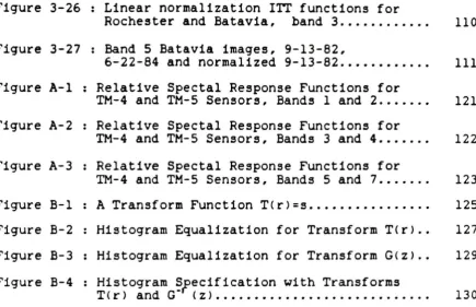
distribution is located. Figure 2-6 illustrates a sample

histogram and the resulting histogram after the 90%

thresholding. This interval was chosen such that errors

introduced _by noise, in the form of variant features or

mixed pixels, which would dominate the signal at the tails

HISTOGRAM OF SEGMENTED PIF

BAND 4 9-13-82

CD CC

QO UJ tNI

o

O^"^^^^p^w^tt^^w^wji

vy

0 20 40 60 80 100 120 140 160 180 200

DIGITAL COUNT

(a)

HISTOGRnM OF SEGMENTED PIF BAND 4 9-13-82

O- i i i i i i i i'i _| i i i i _f i i '

| I I i

| i i