Reducing sequence risk using trend following and the CAPE ratio

City, University of London Institutional Repository

Citation:

10.2469/faj.v73.n4.5

This is the accepted version of the paper.

This version of the publication may differ from the final published

version.

Permanent repository link:

Link to published version:

Copyright and reuse: City Research Online aims to make research

outputs of City, University of London available to a wider audience.

Copyright and Moral Rights remain with the author(s) and/or copyright

holders. URLs from City Research Online may be freely distributed and

linked to.

City Research Online: http://openaccess.city.ac.uk/ [email protected]

1

Reducing sequence risk using trend

following and the CAPE ratio

Andrew Clare

Chair in Asset Management, Cass Business School, City, University of London, London, UK.

James Seaton

Research Fellow, Cass Business School, City, University of London, London. UK.

Peter N. Smith

Chair in Economics and Finance, Department of Economics & Related Studies, University of York, York, UK.

Stephen Thomas

Chair in Finance, Cass Business School, City, University of London, London, UK.

Financial Analysts Journal, Forthcoming

This Version: May 2017

Abstract

The risk of experiencing bad investment outcomes at the wrong time, or sequence risk, is a poorly understood, but crucial aspect of the risk faced by investors, in particular those in the decumulation phase of their savings journey, typically over the period of retirement financed by a defined contributions pension scheme. Using US equity return data from 1872-2014 we show how this risk can be significantly reduced by applying trend-following investment strategies. We also demonstrate that knowledge of a valuation ratio such as the CAPE ratio at the beginning of a decumulation period is useful for enhancing sustainable investment income.

Keywords: Sequence Risk; Perfect Withdrawal Rate; Decumulation; Trend Following; CAPE

2

The topic of pension saving and decumulation is of growing importance in many parts of the

world as companies retreat from defined benefit (DB) schemes leaving investment and

withdrawal decisions to individuals. Some economists have focussed their attention on this

important topic by proposing ever more creative accumulation and decumulation strategies.

These strategies include frameworks for combining deferred annuities, state benefits,

guaranteed annuity-type income, along with flexible income sourced from differing degrees of

risky investment. However, these approaches are generally silent on the type of investment

strategy needed for a successful accumulation and decumulation experience with risky assets.

Instead, they have preferred to create risk-free benchmarks of index-linked bonds (see Sexaeur,

Peskin and Cassidy (2012)). In our view, designing a savings and decumulation strategy

without giving careful consideration to investment strategy is like designing all of the necessary

elements of a car – chassis, gear box, braking system, etc – except the engine.

In this paper we want to shift the focus back to investment strategy – the risk engine. We make

use of the concept of Perfect Withdrawal Rates (PWR) (Suarez et al, 2015) to investigate the

decumulation experience since 1872 of a US investor with a 20-year investment horizon. We

also explain and highlight the potentially pernicious impact that the sequence of investment

returns can have when investors are withdrawing regular income from their investments. This

is known as Sequence Risk. We find evidence to suggest that the application of a simple trend

following filter to an equity investment can help generate returns with low drawdowns which,

in turn, reduces sequence risk leading to enhanced PWRs. Another question that we address

here is whether indicators of equity market valuation are useful for predicting the withdrawal

rates at any point in time. In other words, does, say, a high cyclically-adjusted Shiller PE ratio

3

returns, leading to subsequent lower future PWRs? We find clear evidence to suggest that the

CAPE can be used to help enhance withdrawal rates.

Withdrawal rates

The literature on optimal withdrawal rates in retirement can be traced back to Bengen (1994),

where he presents the concept of “the 4% rule”. Bengen shows that a 4% withdrawal rate from

a retirement fund, adjusted for inflation, is ‘usually’ sustainable for ‘normal’ retirement

periods. Cooley, Hubbard, and Walz (1998, 1999, 2003, and 2011) then confirmed this

conclusion, with similar findings using overlapping samples of historical stock and bond

returns.

A crucial distinguishing feature of these papers is that they rely on a constant real withdrawal

amount throughout the decumulation phase, with no ‘adaptive’ behaviour as circumstances

change. A number of studies have introduced ‘adaptive’ rules: Guyton and Klinger (2006)

manipulate the inflationary adjustment when return rates are too low, modifying the withdrawal

amount, while Frank, Mitchell, and Blanchett (2011) use adjustment rules that depend on how

much the rate of return deviates from the historical averages. Zolt (2013) similarly suggests

curtailing the inflationary adjustment to the withdrawal amount in order to increase the

portfolio’s survival rate where appropriate. Basically these withdrawal rates ‘adapt’ to

changing circumstances.

An important extension of this research is to treat the planning horizon length as a stochastic

variable (instead of fixed). The aim here (quite sensibly!) is to ensure that the funds in the

retirement account “outlive” the retiree: Stout and Mitchell (2006) use mortality tables to make

4

withdrawal amount whenever the account balance falls below a measure of the present value

of the withdrawals yet to be made and increases it when the balance is above this measure.

Mitchell (2011) similarly uses thresholds to initiate such adjustments.

A more theoretically coherent approach treats the selection of withdrawal amounts as a

lifetime-utility maximization problem. Milevsky and Huang (2011) consider the total

discounted value of the utility derived across the entire retirement period, where this length of

retirement is a stochastic variable and the subjective discount rate is a given. Williams and

Finke (2011) use a similar model with more realistic portfolio allocations.

Blanchett, Kowara, and Chen (2012) focus on a different concept. In their paper the researchers

measure the relative efficiency of different withdrawal strategies by comparing the actual cash

flows provided by each strategy to the flows that would have been feasible under perfect

foresight, in other words they make use of the concept of a “perfect withdrawal rate”. This

Perfect Withdrawal Rate (PWR) is the withdrawal rate that effectively exhausts wealth at death

(or at the end of a fixed, known period) which can be identified if one had perfect foresight of

all returns over that period. It can therefore be used as a benchmark for comparing competing

investment strategies and for deriving a measure of a crucial risk faced by investors that are

drawing income from investment portfolios: sequence risk. Sequence Risk is the risk of

experiencing bad investment outcomes at the wrong time. Typically the wrong time is towards

the end of the accumulation phase and at the beginning of the decumulation period, that is, it

is symmetric around the time of retirement. Blanchett et al (2012) and Suarez et al (2015)

construct a probability distribution for the PWR and use it to derive a new measure of sequence

risk in the process. We use these ideas to show that a particular class of investment strategies

5

Withdrawal Rates across virtually the whole range of return’ environments. It is this smoothing

of returns that leads to a better decumulation experience across virtually all investing

timeframes.

Calculating PWRs and deriving a measure of Sequence Risk

For any given series of annual returns there is one and only one constant withdrawal amount

that will leave the desired final balance on the account after n years (the planning horizon).

This is known as the Perfect Withdrawal Amount (PWA). It can also be expressed as a

percentage relative to the initial value of the investment pot, in which case it is referred to as

the Perfect Withdrawal Rate (PWR). The final balance could be a bequest or indeed could be

zero. In the case of the latter, Suarez et al (2015) point out that identifying the PWR is

equivalent to finding the fixed payment that will fully pay off a variable-rate loan after n years.

The basic relationship between account balances in consecutive periods is:

Ki+1 = (Ki - w) (1+ri) (1)

where Ki is the balance at the beginning of year i, w is the yearly withdrawal amount, and ri is

the rate of return in year i in annual percent. Applying equation (1) chain-wise over the entire

planning horizon (n years), we obtain the relation between the starting balance KS (or K1) and

the end balance KE (or Kn):

KE= ({[(KS - w) (1+r1) - w] (1+r2) - w} (1+r3) … - w) (1+rn) (2)

And we solve equation (2) for w to get:

𝑤 = [𝐾𝑆∏𝑛𝑖=1(1 + 𝑟𝑖) − 𝐾𝐸]/ ∑𝑛𝑖=1∏ (1 + 𝑟𝑛𝑗=𝑖 𝑗) (3)

Equation (3) provides the constant amount that will draw the account down to the desired final

6

the second year, minus 6% in the third year, etc., or any other particular sequence of annual

returns. This is the Perfect Withdrawal Amount (PWA).

Quite simply, if one knew in advance the sequence of returns that would come up in the

planning horizon, one would compute the PWA, withdraw that amount each year, and reach

the desired final balance exactly and just in time.

Numerous studies provide examples of a sequence of, say, 30 years of returns generated

possibly with reference to an historical period or via Monte Carlo simulations, and offer the

unique solution of the PWA. It involves withdrawing the same amount every year, giving the

desired final balance with no variation in the income stream, no failure and no surplus. As we

noted above, Blanchett et al (2012) present a measure similar to PWA called the Sustainable

Spending Rate (SSR). Suarez et al (2015) point out that the PWA is a generalization of SSR,

with SSR being the PWA when the starting balance is $1 and the desired final balance is zero.

So every sequence of returns is characterised by a particular PWA, or PWR and hence the

retirement withdrawal question is really a matter of “guessing” what the PWA will turn out to

be (eventually) for each retiree’s portfolio and objectives. So the problem now becomes how

to estimate the probability distribution of PWAs from the probability distribution of the returns

on the assets held in the retirement account.

Note that the analysis so far offers a number of useful insights into sequence risk measurement.

First, Equation (3) can be restated in a particularly useful way since the term ∏𝑛_𝑖=1(1 + 𝑟_𝑖) in the numerator is simply the cumulative return over the entire retirement period, (call it Rn).

7

∑𝑛𝑖=1∏ (1 + 𝑟𝑛𝑗=𝑖 𝑖) = (1+r1)(1+r2)(1+r3)…(1+rn) + (1+r2)(1+r3)…(1+rn) +

(1+r3)(1+r4)…(1+rn) + …. + (1+rn-1)(1+rn) + (1+rn) (4)

The interpretation of this is straightforward: for any given set of returns equation (4) is smaller

if the larger returns occur early in the retirement period and lower rates occur at the end. This

is because the later rates appear more often in the expression. Suarez et al (2015) suggest the

use of the reciprocal of equation (4) to capture the effect of sequencing: so let 𝑆_𝑛 =

1/ ∑ ∏ (1 + 𝑟𝑛 _𝑖

𝑗=𝑖 )

𝑛

𝑖=1 . This falls as the sequence becomes more favourable, and even though

one set of returns appearing in 2 different orders will have the same total return (i.e. Rn with

different Snvalues), so the PWA rates will be different.

Normally the financial analysis of investment returns focus on total return and some reward to

risk measure such as the Sharpe ratio where there is no consideration of the return sequence.

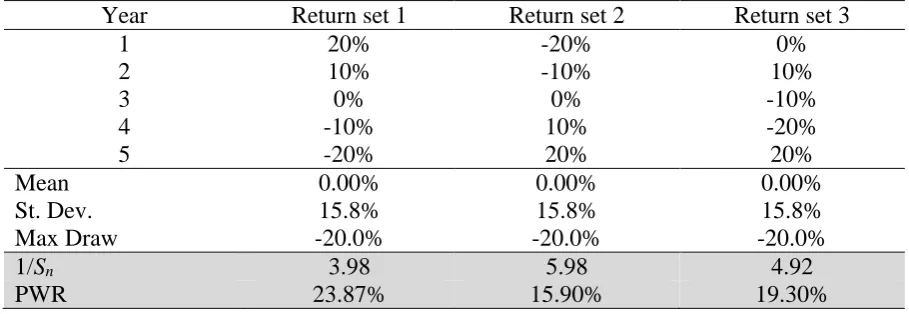
But in both accumulation and decumulation the order of returns matters. An example will make

this clearer. Consider the three sets of returns presented in Table 1; clearly the mean, volatility

and Sharpe (and indeed Maximum Drawdown) are the same in each case, but the returns’

sequence differ as is evidenced by the different values of Sequence Risk (1/Sn) with lower

values of this metric associated with higher PWRs.

This allows a useful, highly intuitive simplification of equation (3) in the form of equation (5),

such that the PWA depends positively on total return, Rn, the starting amount, Ks, and the

measure of sequence risk, Sn, and negatively on the final amount, KE:

8

Table 1 and equation 5 make it clear that it is not simply the total return that matters but the

order in which the component returns occur: if ‘good’ returns come early in the sequence then

the PWA will be larger than if they occur later.

Other studies have tried to account for sequence risk (Frank and Blanchett, 2010; Frank,

Mitchell, & Blanchett, 2011; Pfau, 2014), often developing proxy variables to measure the

correction required due to the sequencing issue. Suarez et al (2015) suggest that equation (5)

comes directly from the simplest, most natural interpretation of the problem, that is that Sn is

not a proxy but a measure of what they term ‘orientation’ (return rates going up, going down,

up a little then down a lot, etc.), and this is the crucial concept for assessing sequencing.

Finally we should note that w (the PWA) can be transformed into a withdrawal rate by dividing

equation (5) by Ks

w/Ks = RnSn - Sn(KE / KS) (6)

Note that if we have a bequest motive then we simply need to know the fraction of the initial

sum to be bequeathed to calculate the PWR. As Suarez et al (2015) point out, in contrast to

simplistic financial planning solutions, to set aside a bequest sum beforehand is not necessary

as these funds can also generate returns and be used for consumption. Setting aside a sum is

simply a special case of the above general form expressed in equation (6).

In this paper we make use of the concept of PWRs to compare investment strategies over a 20

year decumulation horizon. But of course, not everyone will live for twenty years in retirement.

First, it is important to point out that the analysis that we conduct can be adapted for any

withdrawal horizon. But second, and more importantly, we are not suggesting that the

9

that the investment strategies that we investigate should be combined with, say, a deferred

annuity that kicks in at the end of the chosen decumulation period (see for example Merton,

2014 and Sexauer et al, 2012, for a fuller discussion of the potential benefits of this dual

approach to funding one’s retirement).

Constructing a Probability Distribution for PWRs for an all equity portfolio

Much of the financial planning literature aims to make probability statements regarding the

chance of running out of funds given any particular withdrawal rate and planning horizon. So

we now create a probability distribution for the PWR/PWA using a long-run of monthly equity

returns extracted from the Shiller website1. This all-equity portfolio may be considered rather

unlikely as an investment choice in practice, but it serves to illustrate our key points regarding

the choice of investment strategy. In practice of course investors may wish to hold a proportion

in bonds and other asset classes to benefit from diversification and to align the investment

portfolio’s risk to levels of risk tolerance. A surprising result may well be that a 100% equity

portfolio is not such a bad idea, providing that one overlays it with trend-following filter.

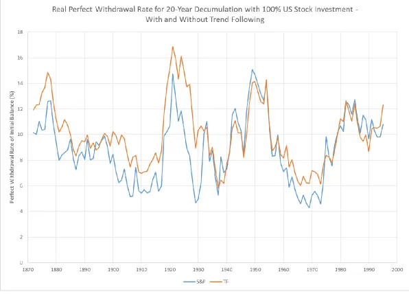
Assuming that we have perfect foresight, what would the real PWR look like through time

assuming a 20 year decumulation period? This is shown in Figure 1 where, as throughout this

paper, we assume a zero bequest intention. We focus here on the blue line which shows the

PWR generally varying between 8% and 12%, but occasionally straying as low as 4% in 1930

and as high as 15% in 1949. For several years in the 1980s it is well above 10%. This suggests

two things. First, there is a huge variation in the ability to withdraw cash from a retirement pot

10

depending on the accident of one’s birth date. Second, all of the rates are above 4%, giving

very long term succour to Bengen’s (1994) 4% rule (at least over 20 year periods).

Now we know what the history of PWRs would look like with perfect foresight for the 100%

S&P500 portfolio, we can construct a probability distribution for this particular investment

strategy. We begin with 100% invested in this equity portfolio. We calculate the real returns

on the S&P500 for each year over the period 1872 to 2014. We then use Monte Carlo

techniques to draw 20 years of return, one at a time, with replacement. These sets of return are

then interpreted as the real returns over a 20-year investment horizon, in the order in which

they were drawn, that an investor might experience. This process is repeated 20,000 times,

allowing us to compute the cumulative return (Rn) and sequencing factor (Sn) for each series of

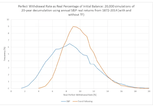
returns obtained. This provides us with 20,000 (Rn, Sn) pairs. The blue line in Figure 2 presents

the frequency distribution of the PWA formula (equation (5)) evaluated at each of these 20,000

(Rn, Sn) pairs, using $100,000 as a starting balance and with $0 as a desired terminal balance.

The second column in Panel A of Table 2 contains the distribution’s percentiles. Taken

together these results are broadly comparable with Figures 3 and 4 in Suarez et al (2015), albeit

with real PWRs and a 20 year investment horizon. We can interpret the distribution of PWRs

as follows: there is a 1% chance of a real PWR of 2.95% or less; a 10% chance of a real PWR

of 5.01% or less; and a 50% chance of a real PWR of 8.64% or more. Given that the final

amount is $0, any overshoot in withdrawing results in ruin. Hence we could say that 50% of

the Monte Carlo withdrawal runs produced real PWRs less than 8.64% so that failure risk for

withdrawing over 8.64% is 50%. Similarly failure risk for withdrawing over 5% p.a. is about

10% (i.e. 10% of runs produced real PWRs of over 5.01%).

The inverse of failure risk is surplus risk and this can be estimated by inverting the roles of

11

a certain percentage of time reflecting the occurrence of PWRs greater than that chosen. In fact,

in the Suarez et al example, with a nominal perfect withdrawal amount of $43,000 p.a. (i.e. a

4.3% withdrawal rule in their case), 74% of the Monte Carlo runs end up with more money

than they began with; in 58% of the runs the final balance was double the starting balance; and

it would have a 12% probability of ending up with 10 times the initial sum.

Finally, in column 2, Panel B of the table we present some descriptive statistics for the real,

buy-and-hold, annual returns on the S&P500 over this period, that is, the descriptive statistics

of the risk engine. Note in particular the very high maximum drawdown of 76.8%.

Trend Following and Sequence Risk

Clearly from equations (6) and (7) the sequence risk measure, Sn, influences the PWR directly:

equation (6) shows that the more favourable sequencing, Sn, gives a higher PWR. More

favourable sequencing is associated with relatively good returns early in the planning period

(see Okusanya (2015)). In particular, the avoidance of heavy losses in the early phases of

decumulation is crucial for high PWAs. But if asset returns are unpredictable, how can we

secure a favourable Sn? Milevsky and Posner (2014) investigate how and when traded equity

options can help reduce sequence risk and, in so doing, be used to extend the life of a retiree’s

investments. However, another very straightforward solution is to acknowledge that while the

order of returns cannot be predicted, it may be possible to produce investment strategies that

offer substantially reduced return volatility or, more precisely, much reduced drawdown in

returns since reduced volatility in itself is not enough to secure a high PWA. Indeed, while

there is no precise mathematical relationship between maximum drawdown and sequence risk

we suggest that a low maximum drawdown should be associated in practice with more

12

While diversifying across asset classes should nudge portfolio returns in the desired direction

with improved risk-return, and possibly lower maximum loss experiences, there is an even

more powerful technique which can be applied to individual asset classes with dramatic effect:

this is ‘trend-following’, where one invests in an asset when it is in an uptrend (defined as a

current value above some measure of recent past average) and switch into cash when the current

value is below such an average2. This approach to investing has been explored by a number of

researchers in the past. Faber (2007) shows how this simple approach can be applied across a

range of broad US asset classes as a disciplined way of implementing asset allocation decisions

to produce multi-asset class portfolios with higher returns and lower volatility3. ap Gwilym et

al (2010) also find that trend following filters can enhance risk-adjusted returns. For example,

they show how the approach can halve the maximum drawdown on an investment in the MSCI

World index, compared to a simple buy-and-hold strategy over the period 1971 to 2008. Hurst

et al (2012) expand the universe of asset classes considerably in their research into the

properties of trend following filters. They apply the trend following filter to 24 commodities

markets, 11 equity markets, 15 bond markets and 9 currency pairs, using data from 1903 to

2012. They find that the approach “delivered strong returns and realized a low correlation

with traditional asset classes” over that period. Clare et al (2013) find similar evidence when

applied to the S&P500, and essentially conclude that the simple ten month moving average

signal4, also applied in this paper, produces superior risk-adjusted returns than more complex

2 _{There is a tendency in the finance industry to use the terms ‘momentum’ and ‘trend following’ almost}

interchangeably, and yet they are subtly different. Trend following, although closely related to momentum investing, originally identified by Jegadeesh and Titman (1993), is fundamentally different in that it does not order the past performance of the assets of interest, though it does rely on a continuation of, or persistence in, price behaviour based on some technical rule. Moskowitz et al (2012) refer to the trend following filter that we use here as “time series momentum”, and refer to the Jegadeesh and Titman momentum effects as “cross-sectional momentum”.

3 _{See also Clare et al (2016) for evidence of how trend following filters can be used to enhance asset allocation by}

predominantly reducing maximum drawdowns on portfolios.

4 _{The authors also show that the ten month calculation period for the average is not critical for their results. They}

13

technical rules, such as those relating to cross-over points, and that any positive return

enhancement applying such trend following rules at a daily frequency is nearly always offset

by higher transactions costs.

Our basic hypothesis then is that applying a simple, monthly trend-following rule to any series

of asset returns dampens volatility, typically maintains or increases returns over longer periods,

and substantially reduces maximum drawdown for that series, which should in turn lead to

lower sequence risk5_{. To test this hypothesis we now replace the buy-and-hold equity}

investment strategy with an equity strategy that incorporates a trend following filter. To this

end, we create a set of trend following returns by using a ten month moving average of the

S&P500. At the end of each month if the index value is greater than its ten month moving

average the investor earns the return on the S&P500 in the subsequent month. However, if at

the end of the month the index value is below its ten month moving average the investor,

switches into cash and earns the return on cash in the subsequent month. The trend following

rule therefore switches the investor between equities and cash depending upon the level of the

index relative to its ten month moving average.

The brown line in Figure 1 presents the real PWR through time assuming a 20 year

decumulation period, and assuming perfect foresight. We can see from the chart that it is

generally higher than the equivalent series generated by the equity buy-and-hold risk engine

of the same trend following rule, but for a range of asset classes, Clare et al (2016) also find that the results are not sensitive to the choice of the moving average calculation.

5 _{For trend following filters such as the one used in this paper to produce attractive, risk-adjusted returns by}

14

[the blue line], which is an encouraging start. We now calculate the distribution of the PWR

generated by the trend following equity risk engine, by first calculating the real return achieved

in each calendar year of our sample from applying the trend following filter. We then repeat

the Monte Carlo analysis, but this time drawing from the set of real annual returns generated

by the trend following rule6. The brown line in Figure 2 shows the distribution of the PWRs

generated by the trend following investment strategy. There is a substantial shift to the right in

the distribution compared with the distribution produced by the buy-and-hold equity strategy

(represented by the blue line in Figure 2) and it is much more concentrated around its median

value of circa 9%. The final column in Panel A of Table 2 presents the percentiles of this

distribution and shows that around 90% of the time the PWRs produced by the trend following

risk engine are greater than produced by the equivalent buy-and-hold equity strategy (shown

in the second column in Panel A). In fact at lower probability levels the PWRs are nearly

double those for the 100% buy-and-hold equity strategy.

The final column in Panel B of Table 2 provides summary statistics of the annual real returns

generated by the trend following strategy and gives a clue to the superior PWRs achieved by

using the trend following strategy. The average real return of 8.84% produced by the trend

following strategy compares very favourably with the 6.82% produced by the buy-and-hold

strategy. However, perhaps even more important is the one-third reduction in volatility from

14.29%pa to 9.86%pa, and the halving of maximum drawdown from 76.8% to 34.88%. In

keeping with the findings of previous research in this area, the trend-following filter applied

here reduces both volatility and maximum loss. This in turn leads to a reduction in sequence

6 _{An alternative to the Monte Carlo approach described here would have been to analyse instead the 1,500 unique}

15

risk, allowing for noticeably higher PWRs in virtually all cases except those greater than the

90th _percentile.

But what about transactions costs?

In achieving the lower sequence risk the trend following filter requires that the investment is

switched between the risky asset class, in this case the S&P500, and cash. Before dealing with

the knotty issue of historical transactions costs however, we can first say something about

holding costs. The trend following literature discussed above has found for a wide range of

asset classes and historic investment periods that the trend following filter described here tends

to require investment in the risky asset class for about two thirds of the time, indeed, this is

also our finding for the S&P500 for the period 1872 to 2014. On the assumption that a cash

balance attracts a much lower holding fee than an investment in equities, over the long term an

investor in a trend following portfolio should expect to pay only two thirds of the holding costs

(management fee) that they would otherwise pay as a result of a buy-and-hold strategy in the

same risky asset.

A transactions charge would only be payable in the event of a switch. ap Gwylym et al (2010)

apply the trend following filter used here to the MSCI World index, in dollars, from 1971 to

2008 and report 7 switches (or round trip trades) per decade. We find that the number of

switches for the S&P500 for the nearly 150 year period analysed here was also just under 7 per

decade. With regard to switching costs, Hurst et al (2012) investigate the benefits of trend

following applying the sort of trend following filter used in this paper to a century of US capital

market data, finding that the filter enhances risk-adjusted returns considerably over the last

century or so. In arriving at these results they estimated, and used one way transactions costs

as a proportion of the value of the investment for developed economy equities as being 0.36%,

16

respectively. Finally, in their investigation of trend following using data from 1994 to 2015,

for a range of asset classes, Clare et al (2016) base equity transactions costs on ETF fees, using

a one way transactions cost of 0.20% of the value of the investment and find that the trend

following filters still outperform buy-and-hold comparable investments by an impressive

margin. For example, they find that applying the same, simple 10 month moving average signal

used in this paper that the approach applied to developed economy equities, produced an

annualised return of 8.0%, a Sharpe ratio of 0.79 and a maximum drawdown of 11.6%; whereas

the equivalent buy-and-hold portfolio produced an annualised return of 6.6%, a Sharpe ratio of

0.33 and maximum drawdown of 46.6%.

To add further insight into the possible impact of transactions costs we calculated a

“break-even” switching fee, which we define as: the one-way transaction cost that would equate the

returns on a Trend Following strategy applied to the S&P500 with those produced by a

‘buy-and hold’ investment in the S&P500, over the full sample period. This break-even value turned

out to be 1.35%. To put this into perspective, Hurst (et al) suggest that a one-way transaction

cost of 0.36% should be used for US equities between 1903 and 1992; while Jones (2002)

estimates one-way transactions costs as averaging 0.38% on US stocks between 1900 and 2001.

We recalculated the 20-year Perfect Withdrawal Rates generated by the trend following

strategy applied to the S&P 500. When we set the one-way transaction cost to Hurst et al’s

recommendation of 0.36% we find that the average PWR is 9.68%, compared with the S&P500

Buy and Hold approach which produces a PWR of 8.8%. Finally, since no investors will be

implementing a strategy like this in the past, it is probably pertinent to consider Hurst et al’s

estimate, based on their practical experience, of the one-way transaction costs for trading US

17

So holding costs of trend following strategies are generally two thirds that of a buy-and-hold

equivalent and switches are relatively rare, at least when trend following is applied at the lower,

monthly frequency, and were unlikely to have been high enough to eliminate the benefits of

the trend following approach in the past.

Can Equity Valuation Measures help in securing higher withdrawals?

The relationship between CAPE and PWRs

If a simple trend-following investment strategy facilitates superior withdrawal rates most of

the time, it is natural to ask whether other market timing or valuation indicators can help

identify withdrawal amounts to give similarly “improved” solutions. In particular, measures

such the CAPE ratio (Shiller, 2001) have been shown to have some predictive power for

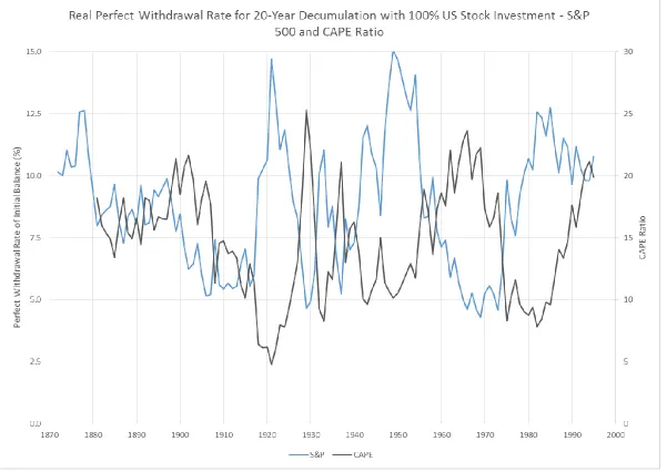
longer-run equity returns7_{. Figure 3 shows the time-series plot of beginning-period CAPE (right-hand}

axis) against the 20-year real PWR generated using by the buy-and-hold equity strategy. If the

earnings’ yield is high (and hence CAPE is low) it is possibly indicative of above average

equity returns and hence we would expect a higher perfect foresight PWR for the subsequent

20-year period. This is seen clearly in Figure 3, with low points for the CAPE in 1920, 1930

and 1980 being associated with high, subsequent PWRs.

We now move on to examine two very different periods of financial market history8, the 20

year period from 1973 and the 20 year period from 1995, to examine in more detail: first, the

potential benefits of updating withdrawal rates on annual basis using our Monte Carlo method;

second, to examine the benefits of trend following in this adaptive PWR framework; and finally

7 _{Blanchett et al (2012) introduce both bond yields and the CAPE ratio as indicators of market valuation.}

8 _{A common feature of the financial planning literature is the analysis of different periods of financial history to}

18

to investigate the possibility of integrating the “predictive” qualities of the CAPE, also updated

annualy.

The period 1995 to 2015

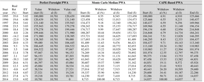
Table 3 presents the results for the 20-year period beginning in 1995 where we use the

buy-and-hold equity portfolio as the risk engine. The second column in the table shows that real

equity returns for the first 5 years of the sample were very high indeed, suggesting the

likelihood of low sequencing risk; this is indeed the case and the perfect foresight, real PWR

is 10.781%, giving a real PWA of $10,781 p.a. for each of the 20 years.

In the columns headed “Monte Carlo Median PWA” in Table 3, we have generated a new,

median PWA for each year in our sample. We do this by applying the Monte Carlo process

described earlier, but on an annual basis to generate the PWA median. More precisely, we

begin by generating the PWR using the Monte Carlo process and 20,000 annual, real return

draws, we then calculate the median of the generated distribution to give the PWA in the first

year (which is $8,545). At the end of the first year we repeat this exercise, but now the

investment horizon is 19, rather than twenty years, so we now draw a series of 19 annual real

returns 20,000 times to create a new distribution and median PWA, and so on. The median

PWA will change each year depending upon the value of the investment pot at the end of the

previous year9. Using this process we can see in Table 3 that after the initial 5 years’ of good

investment performance the investment pot reaches over $188,000 with 16 years to go,

allowing for a withdrawal amount of $19,654. Things then take a turn for the worse in 2008

9 _{We believe that this is a simpler approach to creating adaptive PWAs than the adaptive rules found in the previous}

19

where a 39% fall in the S&P leads to a fall in the PWA from $10,629 to just under $6,000 for

2009 (with 6 years remaining).

The final set of results presented in the columns headed “CAPE-based PWA” are generated by

using the fitted value of the PWR based upon the CAPE at the beginning of each year and the

simple linear regression described above, updated annually to the end of each prior year. The

inverted CAPE values are given in column 3 of the Table (headed “EY”). The fairly low

withdrawal rates in the early years, together with robust investment returns, leads to wealth

reaching over $216,000 by the end of 1999. Together with the CAPE-driven PWRs, this leads

to higher withdrawal amounts in the final years than those suggested by the Monte Carlo

method. For example, the final withdrawal without the CAPE information is $8,715, compared

with $14,037 with it. It would therefore appear then that knowing the value of the CAPE at

the start of the year, could lead to a superior withdrawal experience for investors.

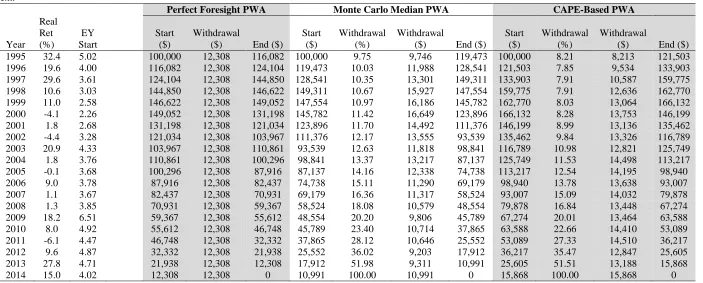
In Table 4 we repeat all of the calculations presented in Table 3 but where the risk engine is

now the trend-adjusted S&P500 real returns. First, we note that the perfect foresight PWR of

12.31% is higher than the 10.78% presented in Table 3. So using trend following filtered

returns leads to a higher PWR, as we have seen previously. Also note how the real returns

generated by the trend-adjusted strategy presented in column 2 of the table, leads to a real return

of -4.4% in 2002 compared to the -22% generated by the buy-and-hold strategy and reported

in column 2 of Table 3, while a real return of 1.3% in 2008 compares favourably to the -39%

generated by the buy-and-hold strategy in the same year. The higher real returns in these two

years in particular facilitate higher PWAs. For example, the withdrawal in 2014 is $10,991

based on the trend following approach compared to $8,715 using the buy-and-hold risk engine.

20

with information from the CAPE. For example the last three withdrawals are $12,847, $13,188

and $15,868 which compare very favourably with the Monte Carlo results produced by the

unadjusted raw equity returns in Table 3 of $6,941, $7,410 and $8,715 respectively.

It would seem then that the trend following approach, combined with the predictive power of

the CAPE together have the potential to produce a much better retirement experience in a

period when raw investment returns are high in the early years.

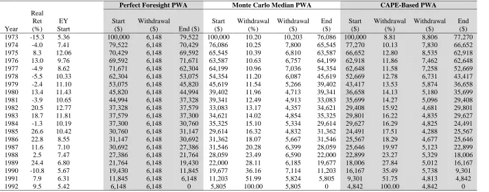
The period 1973 to 1993

What happens if we now repeat this exercise over a period of financial history characterised by

poor returns in the early years, for example the 20 years beginning 1973?

The second column in Table 5 shows real US equity returns for each year from 1973 to 1992.

In 1973 and 1974 real returns were -23% and -34% respectively, suggesting the possibility of

high sequencing risk for anyone starting the decumulation journey in 1973. Although returns

recovered later in the period the damage was done: the perfect foresight PWR, shown in the

table, was only 4.59% for the 20 year period, emphasising that accidents of birth date can have

a major bearing on one’s income in retirement. Both the median Monte Carlo and CAPE

valuation metric produce substantially reduced PWAs relative to those reported in Table 3. For

example, Table 3 shows that the Monte Carlo median approach gives a final withdrawal amount

of $8,715, while the CAPE-based approach yields a final withdrawal value of $14,037; the

equivalent values, shown in Table 5 for the 1973 to 1992 period, are $5,664 and $4,812

21

But what if we now use trend-adjusted equity returns and repeat this exercise over this historical

period? Table 6 contains these results for the trend-adjusted equity returns. First of all note the

absence of really severe negative returns in column 2, which allows the perfect foresight PWR

to rise by a third to 6.148% pa. Similarly the Monte Carlo and CAPE-based results suggest

much higher withdrawals are possible, particularly in the early years, relative to the

trend-unadjusted returns reported in Table 5. However, Table 6 shows that the CAPE-based annual

withdrawals are not as high as those produced by the Monte Carlo approach. In this case then

trend following alone produces the best withdrawal results.

Conclusions

In this paper we have drawn attention to a number of key features of the much neglected

investment aspects of retirement planning and execution. We have also seen how accidents of

birth date can dramatically impact retirement income. While the reduction of sequence risk

may be recognised by financial planning professionals as an important aspect of the

decumulation journey, there is relatively little awareness of it in the mainstream asset

management and investing strategy literature, possibly because there is no widely accepted

measure of it in practice. The challenge of creating investing strategies for the decumulation

phase beyond the risk-free TIPS portfolios of, say, Sexaeur et al (2012), has barely begun: the

choice would seem to be between controlling tail-risk with derivatives (Milevsky and Posner,

2014), versus portfolio timing adjustments into and out of cash (Strub, 2013). This study is

firmly in the latter camp. We show that employing a simple trend following strategy results in

significantly reduced sequence risk while generating a robust level of average returns and

therefore an enhanced feasible withdrawal rate. We also show that there is potentially useful

information in market valuation measures, such as the CAPE ratio, which might help guide

22

The analysis in this paper represents our attempt at identifying a possible risk engine that may

bring investors closer to their own perfect withdrawal rate. However, we acknowledge that

there may well be alternative, superior investment strategies out there. And certainly a process

that encompasses multiple asset classes, rather than just the equity-only approach investigated

here, may provide even better defence against the pernicious effects of sequence risk. We

therefore believe that the research focus should shift to the identification of suitable risk

engines for decumulation journeys. Others have already designed a fine chassis, but a chassis

23

References

ap Gwilym, O., Clare, A., Seaton, J. and S.H. Thomas, (2010), Price and Momentum as Robust Tactical Approaches to Global Equity Investing, The Journal of Investing, Vol. 19, No. 3, 80-91.

Asness, C., Ilmanen, A. and Maloney, T., (2015), Back in the Hunt, Institutional Investor Magazine, November.

Bengen, W. P. (1994), Determining Withdrawal Rates Using Historical Data, Journal of Financial Planning, 7(1), 171-180.

Bernard, G., (2011). Systematic Withdrawal Programs: Unsafe at Any Speed, Journal of Financial Service Professionals, 65, 44-61.

Blanchett, D.M., and L.R. Frank (2009), A Dynamic and Adaptive Approach to Distribution Planning and Monitoring, Journal of Financial Planning 22, 52–66.

Blanchett, D., Kowara, M., and Chen, P. (2012). Optimal Withdrawal Strategy for Retirement Income Portfolios, The Retirement Management Journal, 2, 7-20.

Blanchett D., Finke, M., and Pfau, W.D. (2015). Optimal Portfolios for the Long-Run, mimeo.

Chatterjee, S., Palmer, L., and Goetz, J., (2011). Sustainable Withdrawal Rates of Retirees: Is the Recent Economic Crisis A Cause for Concern? International Journal of Economics and Finance, 3(1), 17-22.

Clare, A., J. Seaton, P.N. Smith and S.H. Thomas, (2013). Breaking in to the Blackbox: Trend Following, Stop Losses and the Frequency of Trading – The Case of the S&P500, Journal of Asset Management, Vol. 14, 182-194.

Clare, A., Seaton, J., Smith, P.N., and Thomas S., (2016). The Trend is Our Friend: Risk Parity, Momentum and Trend Following in Global Asset Allocation, Journal of Behavioral and Experimental Finance. 9, 63-80.

Cooley, P., Hubbard, C., and Walz D., (1998). Retirement Savings: Choosing a Withdrawal Rate that is Sustainable, Journal of the American Association of Individual Investors, 20(2), 16-21.

Cooley, P., Hubbard, C., and Walz D., (1999). Sustainable Withdrawal Rates from Your Retirement Portfolio, Financial Counselling and Planning, 10, 39-47.

Cooley, P., Hubbard, C., and Walz D., (2003). A Comparative Analysis of Retirement Portfolio Success Rates: Simulation Versus Overlapping Periods, Financial Services Review, 12, 115-129.

Cooley, P., Hubbard, C., and Walz D., (2011). Portfolio Success Rates: Where to Draw the Line, Journal of Financial Planning, 24, 48-60.

Faber, M., (2007). A Quantitative Approach to Tactical Asset Allocation, Journal of Wealth Management, 16, 69-79.

Frank, L.R., and Blanchett, D.M., (2010). The Dynamic Implications of Sequencing Risk on a Distribution Portfolio, Journal of Financial Planning, 23, 52-61.

24

Guyton, J. (2004). Decision Rules and Portfolio Management for Retirees: Is the ‘Safe’ Initial Withdrawal Rate Too Safe? Journal of Financial Planning, 17(10), 50-58.

Guyton, J., and Klinger, W., (2006). Decision Rules and Maximum Initial Withdrawal Rates, Journal of Financial Planning, 19(3), 49-57.

Hurst, B., Ooi, Y.H., Pedersen L., (2012), A Century of Evidence on Trend-Following Investing, AQR Capital Management Working Paper.

Jegadeesh, N. and S. Titman, (1993), Returns to Buying Winners and Selling Losers: Implications for Stock Market Efficiency, The Journal of Finance, Vol. 48, No. 1, 65-91.

Jones, C.M. (2002), A Century of Stock Market Liquidity and Trading Costs, working paper, Columbia Business School.

Merton, R.C., (2014). The Crisis in Retirement Planning, Harvard Business Review, July-August.

Milevsky, M. and Huang, H., (2011). Spending Retirement on Planet Vulcan: The Impact of Longevity Risk Aversion on Optimal Withdrawal Rates, Financial Analysts Journal, 67(2), 45-58.

Milevsky, M.A. and Posner, S.E., (2014), Can Collars Reduce Retirement Sequencing Risk? The Journal of Retirement, Spring, 46-56.

Mitchell, J.B., (2009). A Mean-Variance Approach to Withdrawal Rate Management: Theory and Simulation, presented at the Academy of Finance, Chicago, IL: March 19, 2009. http://ssrn.com/abstract=1371695

Mitchell, J.B., (2011). Retirement Withdrawals: Preventative Reductions and Risk Management, Financial Services Review, 20, 45-59.

Moskowitz, T., Ooi, Y. and Pedersen, L. (2012), Time series momentum, Journal of Financial Economics, 104, 228-250.

Okusanya, A., (2015). Pound Cost Ravaging, Aviva for Advisers Paper.

Pfau, W.D., (2014). New Research on How to Choose Portfolio Return Assumptions, Advisor Perspectives, 8, 1-7.

Pye, G.B., (2000). Sustainable Investment Withdrawals, Journal of Portfolio Management, 26, 73-83.

Robinson, C.D., (2007). A Phased-Income Approach to Retirement Withdrawals: A New Paradigm for a More Affluent Retirement, Journal of Financial Planning, 20, 44-56.

Sexauer, S., Peskin, M.W., and Cassidy, D., (2012). Making Retirement Income Last a Lifetime, Financial Analysts Journal, 68(1), 74-84.

Shiller, R., (2001). Irrational Exuberance. Princeton University Press.

Stout, R.G. (2008). Stochastic Optimization of Retirement Portfolios Asset Allocations and Withdrawals, Financial Services Review, 17, 1-15.

25

Strub, I.S., (2013), Tail Hedging Strategies, The Cambridge Strategy (Asset Management) Ltd, mimeo.

Suarez, E.D., Suarez, A. and Walz D.T., (2015), The Perfect Withdrawal Amount: A Methodology for Creating Retirement Account Distribution Strategies, Trinity University Working Paper.

Waring, M.B. and L.B. Siegel, (2015), The Only Spending Rule Article You Will Ever Need, Financial Analysts Journal, January/February 2015, Volume 71, Number 1, 91-107.

Williams, D. and Finke, M.S. (2011). Determining Optimal Withdrawal Rates: An Economic Approach, The Retirement Management Journal, 1(2), 35-46.

26

Table 1

Example of Sequence Risk

In this table we show the impact on Sequence risk (1/Sn) and the Perfect Withdrawal Rate (PWR) of three series

of returns which have the same arithmetic mean (Mean), standard deviation (St. Dev.) and maximum drawdown (Max Draw).

Year Return set 1 Return set 2 Return set 3

1 20% -20% 0%

2 10% -10% 10%

3 0% 0% -10%

4 -10% 10% -20%

5 -20% 20% 20%

Mean 0.00% 0.00% 0.00%

St. Dev. 15.8% 15.8% 15.8%

Max Draw -20.0% -20.0% -20.0%

1/Sn 3.98 5.98 4.92

27

Table 2

Real Perfect Withdrawal Rate Percentiles as a Percentage of Initial Balance

In Panel A of this table, in the column headed “S&P”, we present the percentiles of Perfect Withdrawal Rates (PWRs) for an investor with a twenty year decumulation horizon, a starting investment balance of $100,000 and a desired investment balance of $0, based upon the total returns generated on a buy-and-hold investment in the S&P 500 from 1872 to 2014. Analogous results are presented in the column headed “S&P with trend following”, where the returns have been generated by applying a trend following rule to real S&P returns as described in the text from 1872 to 2014. The distribution on which the percentiles were derived, were generated by Monte Carlo techniques which involved drawing 20 years of 12 monthly return values at random with replacement 20,000 times. Panel B of this Table presents the descriptive statistics of a buy-and-hold investment in the S&P (column headed “S&P”) and for an investment in the S&P where returns have been generated by applying a trend following rule (column headed “S&P with trend following”).

S&P S&P with trend following

Panel A

Percentile % %

1 2.95 5.57

5 4.20 6.61

10 5.01 7.21

20 6.11 8.03

30 7.00 8.67

40 7.85 9.23

50 8.64 9.80

60 9.43 10.38

70 10.38 11.01

80 11.47 11.81

90 13.05 13.00

95 14.37 14.04

99 16.87 16.22

Panel B

Annualized Real Return (%) 6.82 8.84

Annualized Real Volatility (%) 14.29 9.86

28

Table 3

20-Year Decumulation Starting in 1995, based on buy-and-hold S&P 500 real returns

In this Table we present statistics for an investor beginning a 20-year decumulation period beginning in 1995, where investment returns are all driven from a buy-and-hold investment in the S&P500. The second column in the table presents the annual, real return achieved from investing in a buy-and-hold S&P 500 equity portfolio. The third column in the table presents the 1/CAPE value (EY) at the start of each decumulation year. The columns under the heading “Perfect Foresight PWA”, present the value of the investment fund at the start of each year, the annual, perfect foresight withdrawal amount, and the value of the investment fund at the end of each year respectively. The columns under the heading “Monte Carlo Median PWA” present: the value of the investment fund at the start of each year; the annual, perfect foresight withdrawal amount as a proportion of the fund; the cash withdrawal amount; and the value of the investment fund at the end of each year respectively, where the Median PWA has been determined by the Monte Carlo technique described in the text which is applied using data up to the start of the next withdrawal year. The columns under the heading “CAPE-Based PWA” present: the value of the investment fund at the start of each year; the annual, perfect foresight withdrawal amount as a proportion of the fund; the cash withdrawal amount; and the value of the investment fund at the end of each year respectively, where the PWA has been determined at the start of each year by the CAPE regression described in the text.

Perfect Foresight PWA Monte Carlo Median PWA CAPE-Based PWA

Start year Real Ret (%) EY Start Value start ($) Withdraw al ($) Value end

($) Start ($)

Withdraw al (%)

Withdraw

al ($) End ($) Start ($)

Withdraw al (%)

Withdraw

al ($) End ($)

1995 35.0 5.02 100,000 10,781 120,439 100,000 8.55 8,545 123,458 100,000 6.91 6,910 125,666

1996 19.6 4.00 120,439 10,781 131,140 123,458 8.92 11,013 134,473 125,666 6.55 8,233 140,437

1997 29.6 3.61 131,140 10,781 155,943 134,473 9.18 12,340 158,242 140,437 6.59 9,256 169,966

1998 23.5 3.03 155,943 10,781 179,278 158,242 9.58 15,153 176,717 169,966 6.55 11,140 196,154

1999 18.4 2.58 179,278 10,781 199,446 176,717 9.99 17,647 188,287 196,154 6.60 12,956 216,848

2000 -8.8 2.26 199,446 10,781 171,980 188,287 10.44 19,654 153,721 216,848 6.79 14,734 184,241

2001 -14.2 2.68 171,980 10,781 138,385 153,721 10.82 16,625 117,693 184,241 7.51 13,828 146,295

2002 -22.0 3.28 138,385 10,781 99,480 117,693 11.19 13,167 81,489 146,295 8.43 12,333 104,437

2003 20.0 4.33 99,480 10,781 106,445 81,489 11.63 9,476 86,421 104,437 9.71 10,143 113,160

2004 9.3 3.76 106,445 10,781 104,522 86,421 12.46 10,772 82,653 113,160 10.24 11,582 110,983

2005 3.5 3.68 104,522 10,781 97,067 82,653 13.22 10,929 74,269 110,983 11.27 12,504 101,974

2006 11.4 3.78 97,067 10,781 96,153 74,269 14.34 10,652 70,892 101,974 12.55 12,797 99,375

2007 2.1 3.67 96,153 10,781 87,203 70,892 15.70 11,131 61,043 99,375 13.84 13,753 87,458

2008 -39.3 3.85 87,203 10,781 46,397 61,043 17.41 10,629 30,607 87,458 15.53 13,582 44,851

2009 26.6 6.51 46,397 10,781 45,084 30,607 19.57 5,989 31,162 44,851 19.11 8,572 45,924

2010 12.3 4.92 45,084 10,781 38,534 31,162 22.83 7,115 27,014 45,924 21.61 9,922 40,443

2011 -0.8 4.47 38,534 10,781 27,521 27,014 27.82 7,515 19,337 40,443 26.20 10,595 29,600

2012 14.8 4.87 27,521 10,781 19,218 19,337 35.90 6,941 14,230 29,600 34.41 10,187 22,286

2013 27.8 4.71 19,218 10,781 10,781 14,230 52.07 7,410 8,715 22,286 50.71 11,302 14,037

29

Table 4

20-Year Decumulation Starting in 1995, based on real S&P 500 returns with trend following overlay

In this Table we present statistics for an investor beginning a 20-year decumulation period beginning in 1995, where investment returns are all driven by the real return on the S&P500 with a trend following overlay. The second column in the table presents the annual, real return achieved from investing in a buy-and-hold S&P 500 equity portfolio. The third column in the table presents the 1/CAPE value (EY) at the start of each decumulation year. The columns under the heading “Perfect Foresight PWA”, present the value of the investment fund at the start of each year, the annual, perfect foresight withdrawal amount, and the value of the investment fund at the end of each year respectively. The columns under the heading “Monte Carlo Median PWA” present: the value of the investment fund at the start of each year; the annual, perfect foresight withdrawal amount as a proportion of the fund; the cash withdrawal amount; and the value of the investment fund at the end of each year respectively, where the Median PWA has been determined by the Monte Carlo technique described in the text which is applied using data up to the start of the next withdrawal year. The columns under the heading “CAPE-Based PWA” present: the value of the investment fund at the start of each year; the annual, perfect foresight withdrawal amount as a proportion of the fund; the cash withdrawal amount; and the value of the investment fund at the end of each year respectively, where the PWA has been determined at the start of each year by the CAPE regression described in the text.

Perfect Foresight PWA Monte Carlo Median PWA CAPE-Based PWA

Year Real Ret (%) EY Start Start ($) Withdrawal

($) End ($)

Start ($)

Withdrawal (%)

Withdrawal

($) End ($)

Start ($)

Withdrawal (%)

Withdrawal

($) End ($)

1995 32.4 5.02 100,000 12,308 116,082 100,000 9.75 9,746 119,473 100,000 8.21 8,213 121,503

1996 19.6 4.00 116,082 12,308 124,104 119,473 10.03 11,988 128,541 121,503 7.85 9,534 133,903

1997 29.6 3.61 124,104 12,308 144,850 128,541 10.35 13,301 149,311 133,903 7.91 10,587 159,775

1998 10.6 3.03 144,850 12,308 146,622 149,311 10.67 15,927 147,554 159,775 7.91 12,636 162,770

1999 11.0 2.58 146,622 12,308 149,052 147,554 10.97 16,186 145,782 162,770 8.03 13,064 166,132

2000 -4.1 2.26 149,052 12,308 131,198 145,782 11.42 16,649 123,896 166,132 8.28 13,753 146,199

2001 1.8 2.68 131,198 12,308 121,034 123,896 11.70 14,492 111,376 146,199 8.99 13,136 135,462

2002 -4.4 3.28 121,034 12,308 103,967 111,376 12.17 13,555 93,539 135,462 9.84 13,326 116,789

2003 20.9 4.33 103,967 12,308 110,861 93,539 12.63 11,818 98,841 116,789 10.98 12,821 125,749

2004 1.8 3.76 110,861 12,308 100,296 98,841 13.37 13,217 87,137 125,749 11.53 14,498 113,217

2005 -0.1 3.68 100,296 12,308 87,916 87,137 14.16 12,338 74,738 113,217 12.54 14,195 98,940

2006 9.0 3.78 87,916 12,308 82,437 74,738 15.11 11,290 69,179 98,940 13.78 13,638 93,007

2007 1.1 3.67 82,437 12,308 70,931 69,179 16.36 11,317 58,524 93,007 15.09 14,032 79,878

2008 1.3 3.85 70,931 12,308 59,367 58,524 18.08 10,579 48,554 79,878 16.84 13,448 67,274

2009 18.2 6.51 59,367 12,308 55,612 48,554 20.20 9,806 45,789 67,274 20.01 13,464 63,588

2010 8.0 4.92 55,612 12,308 46,748 45,789 23.40 10,714 37,865 63,588 22.66 14,410 53,089

2011 -6.1 4.47 46,748 12,308 32,332 37,865 28.12 10,646 25,552 53,089 27.33 14,510 36,217

2012 9.6 4.87 32,332 12,308 21,938 25,552 36.02 9,203 17,912 36,217 35.47 12,847 25,605

2013 27.8 4.71 21,938 12,308 12,308 17,912 51.98 9,311 10,991 25,605 51.51 13,188 15,868

30

Table 5

20-Year Decumulation Starting in 1973, based on buy-and-hold S&P 500 real returns

In this Table we present statistics for an investor beginning a 20-year decumulation period beginning in 1973, where investment returns are all driven from a buy-and-hold investment in the S&P500. The second column in the table presents the annual, real return achieved from investing in a buy-and-hold S&P 500 equity portfolio. The third column in the table presents the 1/CAPE value (EY) at the start of each decumulation year. The columns under the heading “Perfect Foresight PWA”, present the value of the investment fund at the start of each year, the annual, perfect foresight withdrawal amount, and the value of the investment fund at the end of each year respectively. The columns under the heading “Monte Carlo Median PWA” present: the value of the investment fund at the start of each year; the annual, perfect foresight withdrawal amount as a proportion of the fund; the cash withdrawal amount; and the value of the investment fund at the end of each year respectively, where the Median PWA has been determined by the Monte Carlo technique described in the text which is applied using data up to the start of the next withdrawal year. The columns under the heading “CAPE-Based PWA” present: the value of the investment fund at the start of each year; the annual, perfect foresight withdrawal amount as a proportion of the fund; the cash withdrawal amount; and the value of the investment fund at the end of each year respectively, where the PWA has been determined at the start of each year by the CAPE regression described in the text.

Perfect Foresight PWA Monte Carlo Median PWA CAPE-Based PWA

Year Real Ret (%) EY Start Start ($) Withdrawal

($) End ($)

Start ($) Withdrawal (%) Withdrawal ($) End ($) Start ($) Withdrawal (%) Withdrawal ($) End ($)

1973 -23.5 5.36 100,000 4,591 72,972 100,000 8.84 8,844 69,719 100,000 7.48 7,477 70,765

1974 -34.2 7.41 72,972 4,591 44,987 69,719 8.86 6,178 41,802 70,765 8.79 6,222 42,461

1975 29.1 12.06 44,987 4,591 52,147 41,802 8.87 3,707 49,177 42,461 11.39 4,837 48,568

1976 16.8 9.76 52,147 4,591 55,563 49,177 9.20 4,523 52,172 48,568 10.56 5,130 50,752

1977 -12.2 8.62 55,563 4,591 44,759 52,172 9.62 5,019 41,405 50,752 10.33 5,245 39,960

1978 -1.1 10.33 44,759 4,591 39,728 41,405 9.87 4,089 36,907 39,960 11.57 4,623 34,949

1979 4.3 11.10 39,728 4,591 36,646 36,907 10.25 3,782 34,548 34,949 12.41 4,336 31,928

1980 15.7 11.43 36,646 4,591 37,102 34,548 10.76 3,717 35,684 31,928 13.11 4,185 32,110

1981 -10.5 10.65 37,102 4,591 29,102 35,684 11.42 4,076 28,293 32,110 13.31 4,273 24,918

1982 14.8 12.77 29,102 4,591 28,142 28,293 12.09 3,422 28,555 24,918 15.24 3,796 24,250

1983 18.7 11.81 28,142 4,591 27,948 28,555 13.02 3,719 29,474 24,250 15.56 3,774 24,299

1984 0.7 10.19 27,948 4,591 23,532 29,474 14.14 4,168 25,493 24,299 15.57 3,783 20,669

1985 26.6 10.42 23,532 4,591 23,970 25,493 15.45 3,939 27,278 20,669 16.92 3,496 21,732

1986 22.8 8.55 23,970 4,591 23,793 27,278 17.21 4,695 27,725 21,732 17.48 3,799 22,016

1987 -4.3 7.10 23,793 4,591 18,367 27,725 19.62 5,438 21,318 22,016 18.93 4,167 17,073

1988 13.8 7.47 18,367 4,591 15,674 21,318 22.82 4,864 18,718 17,073 22.33 3,813 15,085

1989 24.4 6.80 15,674 4,591 13,790 18,718 27.72 5,189 16,833 15,085 26.85 4,050 13,731

1990 -8.0 5.67 13,790 4,591 8,466 16,833 35.86 6,036 9,937 13,731 34.37 4,719 8,293

1991 18.4 6.31 8,466 4,591 4,591 9,937 51.87 5,154 5,664 8,293 51.01 4,231 4,812

31

Table 6

20-Year Decumulation Starting in 1973, based on real S&P 500 returns with trend following overlay

In this Table we present statistics for an investor beginning a 20-year decumulation period beginning in 1973, where investment returns are all driven by the real return on the S&P500 with a trend following overlay. The second column in the table presents the annual, real return achieved from investing in a buy-and-hold S&P 500 equity portfolio. The third column in the table presents the 1/CAPE value (EY) at the start of each decumulation year. The columns under the heading “Perfect Foresight PWA”, present the value of the investment fund at the start of each year, the annual, perfect foresight withdrawal amount, and the value of the investment fund at the end of each year respectively. The columns under the heading “Monte Carlo Median PWA” present: the value of the investment fund at the start of each year; the annual, perfect foresight withdrawal amount as a proportion of the fund; the cash withdrawal amount; and the value of the investment fund at the end of each year respectively, where the Median PWA has been determined by the Monte Carlo technique described in the text which is applied using data up to the start of the next withdrawal year. The columns under the heading “CAPE-Based PWA” present: the value of the investment fund at the start of each year; the annual, perfect foresight withdrawal amount as a proportion of the fund; the cash withdrawal amount; and the value of the investment fund at the end of each year respectively, where the PWA has been determined at the start of each year by the CAPE regression described in the text.

Perfect Foresight PWA Monte Carlo Median PWA CAPE-Based PWA

Year Real Ret (%) EY Start Start ($) Withdrawal

($) End ($)

Start ($) Withdrawal (%) Withdrawal ($) End ($) Start ($) Withdrawal (%) Withdrawal ($) End ($)

1973 -15.3 5.36 100,000 6,148 79,522 100,000 10.20 10,203 76,086 100,000 8.81 8,806 77,270

1974 -4.0 7.41 79,522 6,148 70,429 76,086 10.25 7,800 65,545 77,270 10.13 7,830 66,652

1975 8.3 12.06 70,429 6,148 69,592 65,545 10.39 6,810 63,587 66,652 12.80 8,535 62,918

1976 13.0 9.76 69,592 6,148 71,671 63,587 10.63 6,757 64,199 62,918 11.86 7,462 62,648

1977 -4.9 8.62 71,671 6,148 62,304 64,199 10.96 7,036 54,354 62,648 11.58 7,258 52,669

1978 -5.5 10.33 62,304 6,148 53,075 54,354 11.20 6,087 45,619 52,669 12.78 6,731 43,417

1979 -2.4 11.10 53,075 6,148 45,820 45,619 11.54 5,266 39,402 43,417 13.53 5,874 36,658

1980 13.4 11.43 45,820 6,148 44,994 39,402 11.96 4,713 39,341 36,658 14.13 5,180 35,699

1981 -3.9 10.65 44,994 6,148 37,328 39,341 12.49 4,913 33,083 35,699 14.27 5,096 29,408

1982 20.5 12.77 37,328 6,148 37,579 33,083 13.17 4,357 34,621 29,408 15.92 4,681 29,801

1983 18.7 11.81 37,579 6,148 37,300 34,621 14.02 4,854 35,325 29,801 16.22 4,835 29,627

1984 -1.3 10.19 37,300 6,148 30,760 35,325 15.10 5,334 29,614 29,627 16.29 4,825 24,491

1985 26.6 10.42 30,760 6,148 31,147 29,614 16.32 4,832 31,362 24,491 17.51 4,288 25,567

1986 22.8 8.55 31,147 6,148 30,692 31,362 18.07 5,667 31,546 25,567 18.29 4,677 25,646

1987 11.6 7.10 30,692 6,148 27,386 31,546 20.28 6,399 28,059 25,646 19.97 5,123 22,899

1988 2.5 7.47 27,386 6,148 21,764 28,059 23.49 6,590 22,000 22,899 23.27 5,329 18,006

1989 24.4 6.80 21,764 6,148 19,430 22,000 28.11 6,185 19,677 18,006 27.84 5,012 16,167

1990 -10.8 5.67 19,430 6,148 11,845 19,677 36.16 7,114 11,203 16,167 35.49 5,738 9,301

1991 7.9 6.31 11,845 6,148 6,148 11,203 51.99 5,824 5,805 9,301 51.75 4,813 4,842

32

33

34