A novel approach for protection of radial and meshed microgrids

A NOVEL APPROACH FOR PROTECTION OF RADIAL AND

MESHED MICROGRIDS

S. Mirsaeidi*, X. Dong*, D. Tzelepis

, and C. Booth

*Department of Electrical Engineering, Tsinghua University, Beijing, People’s Republic of China, {m_sohrab, xzdong}@mail.tsinghua.edu.cn

†Department of Electronic and Electrical Engineering, University of Strathclyde, Glasgow, United Kingdom {dimitrios.tzelepis, campbell.d.booth}@strath.ac.uk

Keywords: Micro-grid, grid-connected mode, islanded mode,

protection scheme, positive-sequence component.

Abstract

During grid-connected operation mode of microgrids, since the main grid provides a large short-circuit current to the fault point, the protection can be performed by the conventional protective devices, but in islanded mode, fault currents are drastically lower than those of grid-connected mode. Hence, employment of traditional overcurrent-based protective devices in micro-grids is no longer valid and some alternative protection schemes should be developed. This paper presents a micro-grid protection scheme based on positive-sequence component using Phasor Measurement Units (PMUs) and a Central Protection Unit (CPU). The salient feature of the proposed scheme in comparison with the previous works is that it has the ability to protect both radial and meshed micro-grids against different types of faults. Furthermore, since the CPU is capable of updating its pickup values (upstream and downstream equivalent positive-sequence impedances of each line) after the first change in the micro-grid configuration (such as transferring from grid-connected to islanded mode and or disconnection of a line, bus, or DER either in grid-connected mode or in islanded mode), it can protect micro-grid against subsequent faults. In order to verify the effectiveness of the proposed scheme and the CPU, several simulations have been undertaken by using DIgSILENT PowerFactory and MATLAB software packages.

1 Introduction

The manifested merits of Distributed Energy Resources (DERs) in power systems have given rise to significant interests in microgrid development at regional levels. The generation of microgrid had a great influence on the protection of distribution network. The two-way flow characteristics makes it difficult to ensure the selectivity of the protection. The short circuit fault current is also drastically different between grid connected and islanded mode, which makes the conventional schemes unable to protect microgrids [1, 2]. The structure of a typical micro-grid is shown in Figure 1.

The research of microgrid protection has been a hot topic in recent years. In a study by Oudalov and Fidigatti [3], an

transformers) inside the micro-grid. This paper presents a micro-grid protection scheme based on positive-sequence component using PMUs and a CPU. The proposed scheme has the ability to protect both radial and looped micro-grids against different types of faults. Furthermore, since the CPU is capable of updating its pickup values (upstream and downstream equivalent positive-sequence impedances of each line) after the first change in the micro-grid configuration, it can protect micro-grid against subsequent faults.

Figure 1: Structure of a typical micro-grid

2 The proposed protection scheme

This paper presents a protection scheme for micro-grids using PMUs and a CPU, thereby detecting different kinds of faults in both grid-connected and islanded modes of operation. In the proposed protection scheme, PMUs which are responsible for extracting voltage and current phasors (magnitudes and their respective phasor angles) based upon digital sampling of Alternating Current (AC) waveforms, are installed at both ends of each line of micro-grid. Subsequently, the information extracted by PMUs of each line is transferred to the CPU through a digital communication system. After a fault incident within the micro-grid, the information received by PMUs in the CPU is analyzed, and then the fault occurrence, location of fault, and faulted phases are recognized. Finally, depending on the fault type, proper tripping signals are issued to the relevant circuit breakers.

2.1 Detection of fault incident

In order to detect different types of faults, this paper presents a protection scheme based on symmetrical components

approach. The approach, developed by C. L. Fortescue, is one of the most effective ones, applied to transform a three-phase unbalanced system into three sets of symmetrical balanced phasors, namely positive-, negative- and zero- sequence components. In case a fault strikes within a network, these symmetrical components are formed depending on the fault type. However, the positive-sequence is the only component which exists in all types of faults. For this reason, in this study, the positive-sequence component is employed to detect different kinds of faults.

2.2 Detection of fault location

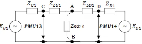
As mentioned earlier, the majority of the proposed methods to date are strongly dependent on the micro-grid configuration. In order to possess an appropriate method having the ability to protect different micro-grids with different configurations, micro-grid feeders should be sectionalized in such a way that each section (micro-grids line or bus) is protected independent of other sections. To fulfill this, the upstream and downstream of each line are replaced with its upstream and downstream equivalent circuits, respectively. Both of these equivalent circuits include a voltage source in series with impedance. Figure 2 indicates the upstream and downstream equivalent circuits of Line12 of Figure 1 during a fault.

Figure 2: Upstream and downstream equivalent circuits of Line12 of Figure 1 during a fault

During a fault occurrence in Line 12 of Figure 1, different symmetrical components are created depending on the fault type. By replacing the equivalent impedance of negative- and zero- sequence networks between terminals AB of positive-sequence network for all types of faults, a general model for the analysis of different kinds of faults can be developed. The developed model is demonstrated in Figure 3, in which impedance 𝑍𝑒𝑞2,0 is the representative of negative- and zero-

sequence networks.

Figure 3: Developed general model for the analysis of different kinds of faults

Depending on the fault type, the value of this impedance is different. Equation (1) expresses the value of impedance 𝑍𝑒𝑞2,0

𝑍𝑒𝑞2,0:

{

𝑍𝑒𝑞0+ 𝑍𝑒𝑞2 for single line to ground faults

𝑍𝑒𝑞2 for line to line faults

𝑍𝑒𝑞0‖𝑍𝑒𝑞2 for line to line to ground faults

0 for three phase faults

(1) where,

𝑍𝑒𝑞0= (𝑍𝑈0+ 𝑍𝐿𝑈0)‖(𝑍𝐷0+ 𝑍𝐿𝐷0)

𝑍𝑒𝑞2= (𝑍𝑈2+ 𝑍𝐿𝑈2)‖(𝑍𝐷2+ 𝑍𝐿𝐷2)

In the proposed protection scheme, after the detection of fault incident, the faulted section is recognized by the developed model of Figure 3 in such a way as to compare the value of upstream and downstream equivalent positive-sequence impedances, before and after the fault. In fact, when a fault occurs inside a line, impedance 𝑍𝑒𝑞2,0 is created between points

C and D. Therefore, the values of both upstream and downstream equivalent positive-sequence impedances after the fault (𝑍𝑈1, 𝑍𝐷1) remain equal to the values of those impedances

before the fault (𝑍𝑈1 (𝑝𝑟𝑒), 𝑍𝐷1 (𝑝𝑟𝑒)), but in case a fault occurs

at the upstream or downstream of a line, respectively, only the value of 𝑍𝐷1 or only the value of 𝑍𝑈1 remains constant after

the fault.

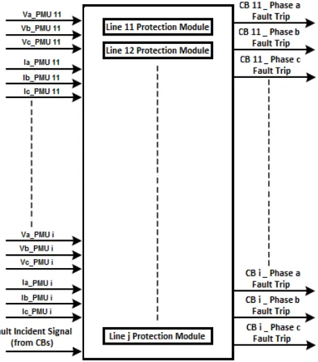
3 Structure of the Central Protection Unit

(CPU)

In order to implement the proposed protection scheme, a digital CPU has been designed. The schematic diagram of the CPU for the micro-grid shown in Figure 1 is demonstrated in Figure 4. As can be seen in the figure, for the protection of each line and its adjacent buses, a specific Protection Module (PM) is dedicated. Each PM receives the voltage and current phasors from the installed PMUs at both ends of the respective line. If the fault occurs inside that line or its adjacent buses, the proper tripping signal commands are sent to the respective circuit breakers, and then the faulted section is isolated from the rest of the micro-grid. Each PM consists of two main parts, namely, fault incident detector and fault locator, which are described in detail in the following subsections:

3.1 Fault incident detector

As explained earlier, the positive-sequence component is the only component which exists in all types of faults. Therefore, in the proposed protection scheme, the component is used to detect different kinds of faults. When a fault occurs in a micro-grid section (line or bus), the positive-sequence current magnitude of that section is drastically increased; hence, the fault occurrence can be detected by comparing the magnitude before and after the fault. In the CPU, this function is performed by fault incident detector. It should be noted that the settings of the fault incident detector should be such a way as to avoid the mal-operation of the PMs in case of a small change in the positive-sequence current magnitude. Moreover, since a fault in one section may increase the positive-sequence current magnitude of other sections, PMs related to non-faulted lines in the CPU may issue fault trip signals mistakenly. Hence, the

deployment of an additional detector (Fault locator) is necessary.

Figure 4: Schematic diagram of the CPU for the micro-grid shown in Figure 1

3.2 Fault locator

As mentioned in Subsection 2.2, the faulted section is identified based on changes in the values of upstream and downstream equivalent positive-sequence impedances before and after the fault. In the CPU, this function is performed by fault locator. Prior to fault incident, the fault locator respective to each line, first, calculates the values of Thevenin’s Equivalent Positive-Sequence Impedances (TEPSIs) at both ends of that line, and then it deploys the values to determine the values of impedances 𝑍𝑈1 (𝑝𝑟𝑒) and 𝑍𝐷1 (𝑝𝑟𝑒). Finally, the

faulted section can be recognized by comparing the values of upstream and downstream equivalent positive-sequence impedances before (𝑍𝑈1 (𝑝𝑟𝑒), 𝑍𝐷1 (𝑝𝑟𝑒)) and after (𝑍𝑈1, 𝑍𝐷1)

the fault.

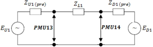
Figure 5: Equivalent circuit diagram of the positive- sequence network for Line 12 (of Figure 1) prior to fault occurrence Based on Thevenin’s model, the node positive-sequence voltage equation is defined as:

𝑉1= 𝐸𝑡1− 𝑍𝑡1∙ 𝐼1 (2)

According to Equation (2), the positive-sequence voltage equation for PMU13 terminals becomes:

𝑉1𝑃𝑀𝑈13= 𝐸𝑡1𝑃𝑀𝑈13− 𝑍𝑡1𝑃𝑀𝑈13∙ 𝐼1𝑃𝑀𝑈13 (3)

Where,

𝐸𝑡1𝑃𝑀𝑈13=Thevenin’s equivalent positive-sequence voltage

source at PMU13 terminals

𝑍𝑡1𝑃𝑀𝑈13=Thevenin’s equivalent positive-sequence

impedance at PMU13 terminals

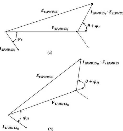
Positive-sequence phasor diagrams of Equation (3) for two different measurements at PMU13 terminals are indicated in Figure 6. Since 𝐸𝑡1𝑃𝑀𝑈13 is the Thevenin’s positive-sequence

equivalent voltage source, its magnitude for both measurements are identical, but its angle in the IInd measurement is shifted by an angle equal to the phase drift. Referring to Figure 6, 𝐸𝑡1𝑃𝑀𝑈13 equation for the Ist

measurement can be written as: 𝐸𝑡1𝑃𝑀𝑈132 = 𝑉1𝑃𝑀𝑈13𝐼

2 _{+ 𝐼}

1𝑃𝑀𝑈13𝐼

2 _{∙ 𝑍}

𝑡1𝑃𝑀𝑈132 + 2𝑉1𝑃𝑀𝑈13𝐼∙

𝐼1𝑃𝑀𝑈13𝐼∙ 𝑍𝑡1𝑃𝑀𝑈13∙ cos(𝜃 + 𝜑𝐼) (4)

By expanding cos(𝜃 + 𝜑𝐼), Equation (4) can be expressed as

follows:

𝐸𝑡1𝑃𝑀𝑈132 = 𝑉1𝑃𝑀𝑈13𝐼

2 _{+ 𝐼}

1𝑃𝑀𝑈13𝐼

2 _{∙ 𝑍}

𝑡1𝑃𝑀𝑈132 + 2𝑃1𝑃𝑀𝑈13𝐼∙

𝑅𝑡1𝑃𝑀𝑈13− 2𝑄1𝑃𝑀𝑈13𝐼∙ 𝑋𝑡1𝑃𝑀𝑈13 (5)

Where 𝑅𝑡1𝑃𝑀𝑈13 and 𝑋𝑡1𝑃𝑀𝑈13 denote the resistance and

reactance of the Thevenin’s equivalent positive-sequence impedance, as well as 𝑃1𝑃𝑀𝑈13𝐼 and 𝑄1𝑃𝑀𝑈13𝐼 , which

respectively represent active and reactive powers flowing through Line 12. Likewise, the 𝐸𝑡1𝑃𝑀𝑈13 equation for the IInd

measurement can be written as: 𝐸𝑡1𝑃𝑀𝑈132 = 𝑉1𝑃𝑀𝑈13𝐼𝐼

2 _{+ 𝐼}

1𝑃𝑀𝑈13𝐼𝐼

2 _{∙ 𝑍}

𝑡1𝑃𝑀𝑈132 + 2𝑃1𝑃𝑀𝑈13_𝐼𝐼∙

𝑅𝑡1𝑃𝑀𝑈13− 2𝑄1𝑃𝑀𝑈13𝐼𝐼∙ 𝑋𝑡1𝑃𝑀𝑈13 (6)

By subtracting Equation (6) from Equation (5):

𝑉1𝑃𝑀𝑈13𝐼

2 _{− 𝑉}

1𝑃𝑀𝑈13𝐼𝐼

2 _{+ (𝐼} 1𝑃𝑀𝑈13𝐼

2 _{− 𝐼}

1𝑃𝑀𝑈13𝐼𝐼

2 _{) ∙ 𝑍}

𝑡1𝑃𝑀𝑈132 +

2(𝑃1𝑃𝑀𝑈13𝐼− 𝑃1𝑃𝑀𝑈13𝐼𝐼) ∙ 𝑅𝑡1𝑃𝑀𝑈13− 2(𝑄1𝑃𝑀𝑈13𝐼−

𝑄1𝑃𝑀𝑈13𝐼𝐼) ∙ 𝑋𝑡1𝑃𝑀𝑈13= 0 (7)

Equation (7) can be arranged as follows:

(𝑅𝑡1𝑃𝑀𝑈13+

𝑃_{1𝑃𝑀𝑈13𝐼}−𝑃_{1𝑃𝑀𝑈13𝐼𝐼} 𝐼_{1𝑃𝑀𝑈13𝐼}2 −𝐼_{1𝑃𝑀𝑈13𝐼𝐼}2 )

2

+ (𝑋𝑡1𝑃𝑀𝑈13−

𝑄_{1𝑃𝑀𝑈13𝐼}−𝑄_{1𝑃𝑀𝑈13𝐼𝐼} 𝐼_{1𝑃𝑀𝑈13𝐼}2 −𝐼_{1𝑃𝑀𝑈13𝐼𝐼}2 )

2

=𝑉1𝑃𝑀𝑈13𝐼𝐼

2 _−𝑉 1𝑃𝑀𝑈13𝐼2

𝐼_{1𝑃𝑀𝑈13𝐼}2 −𝐼_{1𝑃𝑀𝑈13𝐼𝐼}2 +

(𝑃1𝑃𝑀𝑈13𝐼−𝑃1𝑃𝑀𝑈13𝐼𝐼

𝐼

1𝑃𝑀𝑈13𝐼2 −𝐼1𝑃𝑀𝑈13𝐼𝐼2

)

2

+ (𝑄1𝑃𝑀𝑈13𝐼−𝑄1𝑃𝑀𝑈13𝐼𝐼

𝐼

1𝑃𝑀𝑈13𝐼2 −𝐼1𝑃𝑀𝑈13𝐼𝐼2

)

2

(8)

This is the equation of a circle in the positive-sequence impedance plane which indicates a locus for the Thevenin’s equivalent positive-sequence impedance seen from PMU13 terminals. As it does not specify a certain value for 𝑍𝑡1𝑃𝑀𝑈13 ,

a third measurement is required so that it is used with the first and second measurements to create two other circles for 𝑍𝑡1𝑃𝑀𝑈13 . According to Thevenin’s theorem, Thevenin’s

equivalent impedance for any two-terminal of the network is the impedance seen from those terminals when the sources are set to zero. Hence, 𝑍𝑡1𝑃𝑀𝑈13 for PMU13 terminals of Figure 5

is equivalent to 𝑍𝑈1‖(𝑍𝐿1+ 𝑍𝐷1). By setting this equal to the

calculated 𝑍𝑡1𝑃𝑀𝑈13 from the intersection point of the three

circles:

𝑍_{𝑡1𝑃𝑀𝑈13𝑐𝑎𝑙.}= 𝑍𝑈1 (𝑝𝑟𝑒)‖(𝑍𝐿1+ 𝑍𝐷1 (𝑝𝑟𝑒)) (9)

By following the same procedure for PMU14 terminals of Figure 5:

𝑍_{𝑡1𝑃𝑀𝑈14𝑐𝑎𝑙.}= 𝑍𝐷1 (𝑝𝑟𝑒)‖(𝑍𝐿1+ 𝑍𝑈1 (𝑝𝑟𝑒)) (10)

By solving Equations (9) and (10), the values of 𝑍𝑈1 (𝑝𝑟𝑒) and

𝑍𝐷1 (𝑝𝑟𝑒) are obtained. Subsequently, the fault locator

respective to each line compares the values of 𝑍𝑈1 (𝑝𝑟𝑒) and

𝑍𝐷1 (𝑝𝑟𝑒) with the values of 𝑍𝑈1 and 𝑍𝐷1 after the fault incident

and identifies the faulted section.

4 Simulation results

Figure 6: Positive- sequence phasor diagrams for two different measurements at PMU13 terminals: (a) Ist _{measurement (b) II}nd measurement

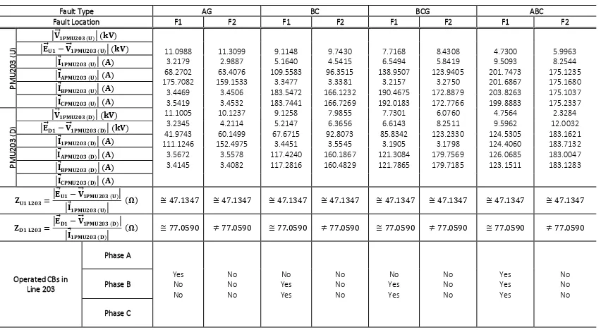
To prove the efficacy of the CPU in the grid-connected and islanded operating modes, the performance of several PMs was simulated using DIgSILENT PowerFactory and MATLAB software packages, but due to space restriction and format requirements of this publication, only the simulation results of Line 203 Protection Module is included in this paper. According to the simulation results, the calculated values of upstream and downstream equivalent positive-sequence impedances (from the intersection of circles) for Line 203 before the fault incidents in both grid-connected and islanded operating modes are as follows:

𝑍_{𝑈1 𝐿203 (𝑝𝑟𝑒)𝑐𝑎𝑙.}: {8.7499 (Ω) for grid − connected mode 47.1347 (Ω) for islanded mode

𝑍_{𝐷1 𝐿203 (𝑝𝑟𝑒)𝑐𝑎𝑙.}: {8.5499 (Ω) for grid − connected mode 77.0590 (Ω) for islanded mode

where,

𝑍_{𝑈1 𝐿203 (𝑝𝑟𝑒)𝑐𝑎𝑙.}= Upstream equivalent positive-sequence impedance of PMU203 (U)

𝑍_{𝐷1𝐿203 (𝑝𝑟𝑒)𝑐𝑎𝑙.}= Downstream equivalent positive-sequence impedance of PMU203 (D)

Tables 1 and 2 indicate the simulation results of Line203 Protection Module during different kinds of faults at the midpoint of Lines 203 and 302 (F1 and F2 in Figure 7) in both grid-connected and islanded operating modes, respectively. As can be seen from the tables, the positive- sequence current magnitudes during different types of faults in islanded mode are drastically lower than those of grid-connected mode. It is due to the fact that the Thevenin’s impedance viewed from the fault points (F1 and F2) in islanded operating mode is much

higher than that in the grid-connected mode; therefore, traditional over-current strategies with a single setting group will not be able to provide a selective trip for all types of faults in both grid-connected and islanded modes of operation. Once fault F1 or F2 occurred either in grid-connected or islanded mode, Line 203 Protection Module calculates the values of 𝑍𝑈1 𝐿203 and 𝑍𝐷1 𝐿203 and then compares them, respectively,

with the values of 𝑍𝑈1 𝐿203 (𝑝𝑟𝑒)_{𝑐𝑎𝑙.} and 𝑍𝐷1 𝐿203 (𝑝𝑟𝑒)_{𝑐𝑎𝑙.}.

According to Tables 1 and 2, since Fault F1 has occurred inside of Line 203, the values of 𝑍𝑈1 𝐿203 and 𝑍𝐷1 𝐿203 are

respectively equal to the values of 𝑍𝑈1 𝐿203 (𝑝𝑟𝑒)𝑐𝑎𝑙. and

𝑍𝐷1 𝐿203 (𝑝𝑟𝑒)𝑐𝑎𝑙., whereas fault F2 has occurred at the

downstream of Line 203 and therefore, only the value of 𝑍𝑈1 𝐿203 is equal to the value of 𝑍𝑈1 𝐿203 (𝑝𝑟𝑒)_{𝑐𝑎𝑙.}.

Figure 7: Single-line diagram of the test micro-grid

5 Conclusion

This paper proposed a protection scheme based on positive-sequence component for micro-grids. In spite of the majority of the developed protection strategies to date which are strongly dependent on the network architecture, the suggested scheme is capable of protecting different micro-grids with different configurations. In fact, the proposed scheme has the ability to protect either radial or meshed micro-grids against different types of faults. Moreover, Since the designed CPU is capable of updating their pickup values after the first change in the micro-grid configuration, it can protect micro-grid lines and buses against subsequent faults.

Acknowledgements

Table 1: The simulation results of Line 203 Protection Module during the grid-connected mode

Table 2: The simulation results of Line 203 Protection Module during the islanded mode

References

[1] A. Hooshyar and R. Iravani, “Microgrid Protection,” Proc.

of the IEEE, vol. 105, no. 7, pp. 1332-1353, (2017).

[2] E. Sortomme, S. S. Venkata and J. Mitra, “Microgrid Protection Using Communication-Assisted Digital Relays, ” in IEEE Transactions on Power Delivery, vol. 25, no. 4, pp. 2789-2796, (2010).

[3] A. Oudalov and A. Fidigatti, “Adaptive network protectionin microgrids,” International Journal of

Distributed Energy Resources, 5, pp. 201-225, (2009).

[4] M. Dewadasa, R. Majumder, A. Ghosh and G. Ledwich, “Control and protection of a microgrid with converter

interfaced micro sources, International Conference on

Power Systems, Kharagpur, pp. 1-6, (2009).

[5] H. Al-Nasseri and M. A. Redfern, “Harmonics content based protection scheme for Micro-grids dominated by solid state converters,” 12th International Middle-East

Power System Conference, Aswan, pp. 50-56, (2008).

[6] H. Nikkhajoei and R. H. Lasseter, “Microgrid Protection,”

2007 IEEE Power Engineering Society General Meeting,

Tampa, FL, pp. 1-6, (2007).

[7] M. A. Zamani, T. S. Sidhu and A. Yazdani, “A Protection Strategy and Microprocessor-Based Relay for Low-Voltage Microgrids,” in IEEE Transactions on Power

Delivery, vol. 26, no. 3, pp. 1873-1883, (2011).

Fault Type AG BC BCG ABC

Fault Location F1 F2 F1 F2 F1 F2 F1 F2

P M U 20 3 (U )

|𝐕⃗⃗ _{𝟏𝐏𝐌𝐔𝟐𝟎𝟑 (𝐔)}| (𝐤𝐕)

11.5966 2.7971 319.6722 930.9764 3.2012 3.2109 11.6082 2.7872 325.9221 930.5706 3.3172 3.3204 11.9350 2.4659 281.8203 782.8649 3.2266 3.2204 10.7275 3.6819 489.6217 1410.6070 3.3023 3.3186 9.6348 4.7554 543.4804 3.1912 940.2354 940.8970 9.6623 4.7308 553.3164 3.1866 959.9520 961.2623 10.3793 4.0319 460.7938 3.18577 794.6089 796.4964 8.0940 6.3265 863.8151 3.1499 1488.0535 1484.2312 8.4334 5.9731 682.6478 3.1100 1001.0088 1002.0910 8.4671 5.9364 694.3239 3.1760 1021.8158 1021.4874 9.3542 5.0408 576.0980 3.1634 821.6507 826.4506 6.4597 8.0298 1118.3574 3.0042 1630.9718 1687.0680 5.5298 8.8869 1015.6570 1023.2251 1032.0562 1014.3305 5.5934 8.8155 1031.0646 1032.2881 1033.3917 1028.5264 7.0634 7.3347 838.2610 840.8320 847.7558 836.2392 2.4528 11.9826 1756.9881 1750.8619 1758.9912 1753.9268

|𝐄⃗ 𝐔𝟏− 𝐕⃗⃗ 𝟏𝐏𝐌𝐔𝟐𝟎𝟑 (𝐔)| (𝐤𝐕)

|𝐈 𝟏𝐏𝐌𝐔𝟐𝟎𝟑 (𝐔)| (𝐀)

|𝐈 𝐀𝐏𝐌𝐔𝟐𝟎𝟑 (𝐔)| (𝐀)

|𝐈 𝐁𝐏𝐌𝐔𝟐𝟎𝟑 (𝐔)| (𝐀)

|𝐈 𝐂𝐏𝐌𝐔𝟐𝟎𝟑 (𝐔)| (𝐀)

P M U 20 3 (D )

|𝐕⃗⃗ _{𝟏𝐏𝐌𝐔𝟐𝟎𝟑 (𝐃)}| (𝐤𝐕) |𝐄⃗ 𝐃𝟏− 𝐕⃗⃗ 𝟏𝐏𝐌𝐔𝟐𝟎𝟑 (𝐃)| (𝐤𝐕)

|𝐈 𝟏𝐏𝐌𝐔𝟐𝟎𝟑 (𝐃)| (𝐀)

|𝐈 𝐀𝐏𝐌𝐔𝟐𝟎𝟑 (𝐃)| (𝐀)

|𝐈 𝐁𝐏𝐌𝐔𝟐𝟎𝟑 (𝐃)| (𝐀)

|𝐈 𝐂𝐏𝐌𝐔𝟐𝟎𝟑 (𝐃)| (𝐀)

𝐙𝐔𝟏 𝐋𝟐𝟎𝟑=

|𝐄⃗ 𝐔𝟏− 𝐕⃗⃗ 𝟏𝐏𝐌𝐔𝟐𝟎𝟑 (𝐔)|

|𝐈 𝟏𝐏𝐌𝐔𝟐𝟎𝟑 (𝐔)|

(𝛀) ≅ 8.7499 ≅ 8.7499 ≅ 8.7499 ≅ 8.7499 ≅ 8.7499 ≅ 8.7499 ≅ 8.7499 ≅ 8.7499 𝐙𝐃𝟏 𝐋𝟐𝟎𝟑=

|𝐄⃗ 𝐃𝟏− 𝐕⃗⃗ 𝟏𝐏𝐌𝐔𝟐𝟎𝟑 (𝐃)|

|𝐈 𝟏𝐏𝐌𝐔𝟐𝟎𝟑 (𝐃)|

(𝛀) ≅ 8.5499 ≠ 8.5499 ≅ 8.5499 ≠ 8.5499 ≅ 8.5499 ≠ 8.5499 ≅ 8.5499 ≠ 8.5499

Operated CBs in Line 203 Phase A Yes No No No No No No Yes Yes No No No No Yes Yes No No No Yes Yes Yes No No No Phase B Phase C

Fault Type AG BC BCG ABC

Fault Location F1 F2 F1 F2 F1 F2 F1 F2

P M U 2 0 3 (U )

|𝐕⃗⃗ _{𝟏𝐏𝐌𝐔𝟐𝟎𝟑 (𝐔)}| (𝐤𝐕)

11.0988 3.2179 68.2702 175.7082 3.4469 3.5419 11.1005 3.2345 41.9743 111.1246 3.5672 3.4145 11.3099 2.9887 63.4076 159.1533 3.4506 3.4532 10.1237 4.2114 60.1499 152.4975 3.5578 3.4082 9.1148 5.1640 109.5583 3.3477 183.5472 183.7441 9.1258 5.2147 67.6715 3.4451 117.4240 117.2816 9.7430 4.5415 96.3515 3.3381 166.1232 166.7269 7.9855 6.3656 92.8073 3.5545 160.1867 160.4829 7.7168 6.5494 138.9507 3.2157 190.4675 192.0183 7.7301 6.6143 85.8342 3.1905 121.3084 121.7865 8.4308 5.8419 123.9405 3.2750 172.8879 172.7766 6.0760 8.2511 123.2330 3.1798 179.7569 179.7185 4.7300 9.5093 201.7473 201.6867 203.8263 199.8883 4.7564 9.5962 124.5305 124.4060 126.0685 123.1511 5.9963 8.2544 175.1235 175.1680 175.1037 175.2337 2.3284 12.0032 183.1621 183.7132 183.0047 183.1283

|𝐄⃗ 𝐔𝟏− 𝐕⃗⃗ 𝟏𝐏𝐌𝐔𝟐𝟎𝟑 (𝐔)| (𝐤𝐕)

|𝐈 𝟏𝐏𝐌𝐔𝟐𝟎𝟑 (𝐔)| (𝐀)

|𝐈 𝐀𝐏𝐌𝐔𝟐𝟎𝟑 (𝐔)| (𝐀)

|𝐈 𝐁𝐏𝐌𝐔𝟐𝟎𝟑 (𝐔)| (𝐀)

|𝐈 𝐂𝐏𝐌𝐔𝟐𝟎𝟑 (𝐔)| (𝐀)

P M U 2 0 3 (D )

|𝐕⃗⃗ _{𝟏𝐏𝐌𝐔𝟐𝟎𝟑 (𝐃)}| (𝐤𝐕) |𝐄⃗ 𝐃𝟏− 𝐕⃗⃗ 𝟏𝐏𝐌𝐔𝟐𝟎𝟑 (𝐃)| (𝐤𝐕)

|𝐈 𝟏𝐏𝐌𝐔𝟐𝟎𝟑 (𝐃)| (𝐀)

|𝐈 𝐀𝐏𝐌𝐔𝟐𝟎𝟑 (𝐃)| (𝐀)

|𝐈 𝐁𝐏𝐌𝐔𝟐𝟎𝟑 (𝐃)| (𝐀)

|𝐈 𝐂𝐏𝐌𝐔𝟐𝟎𝟑 (𝐃)| (𝐀)

𝐙𝐔𝟏 𝐋𝟐𝟎𝟑=

|𝐄⃗ 𝐔𝟏− 𝐕⃗⃗ 𝟏𝐏𝐌𝐔𝟐𝟎𝟑 (𝐔)|

|𝐈 𝟏𝐏𝐌𝐔𝟐𝟎𝟑 (𝐔)|

(𝛀) ≅ 47.1347 ≅ 47.1347 ≅ 47.1347 ≅ 47.1347 ≅ 47.1347 ≅ 47.1347 ≅ 47.1347 ≅ 47.1347 𝐙𝐃𝟏 𝐋𝟐𝟎𝟑=

|𝐄⃗ 𝐃𝟏− 𝐕⃗⃗ 𝟏𝐏𝐌𝐔𝟐𝟎𝟑 (𝐃)|

|𝐈 𝟏𝐏𝐌𝐔𝟐𝟎𝟑 (𝐃)|

(𝛀) ≅ 77.0590 ≠ 77.0590 ≅ 77.0590 ≠ 77.0590 ≅ 77.0590 ≠ 77.0590 ≅ 77.0590 ≠ 77.0590