One size does not fit all... Panel data: Bayesian model
averaging and data poolability
Rodolphe Desbordes
∗Gary Koop
†Vincent Vicard
‡Abstract
We show in this paper why researchers ought to pay particular attention to the issues of model
uncer-tainty and data poolability in their panel data applications. We focus on the identification of robust
deter-minants of current account balances (CABs). Applying Bayesian Model Averaging, we adopt a flexible
modelling approach to highlight that (i) some determinants have limited relevance when accounting for
model uncertainty; (ii) slope homogeneity is unlikely to be a valid assumption; iii) cross-sectional and
time-series relationships can diverge. We explain why estimating cross-sectional estimates is valuable,
even in the potential presence of an omitted variable bias, and suggest a way for assessing the effects of
unobserved country heterogeneity.
Keywords: Bayesian model averaging; current account; heterogeneity; panel data; poolability.
JEL Classification: F32, C11, C21, C23
Word count:7562
∗Corresponding author, SKEMA-UCA. E-mail: [email protected]. Mail: SKEMA Paris, La D´efense Campus,
Pˆole Universitaire L´eonard de Vinci, Esplanade Mona Lisa, Courbevoie, 92916 Paris La D´efense Cedex, France. Phone: +33 (0)1 41 16 74 61.
1
Introduction
Martin Wolf, in his book ‘The Shifts and the Shocks’, describes the global financial crisis and the more
recent Eurozone crisis as being the immediate consequences of global and regional current account
imbal-ances (Wolf, 2014). This interpretation is widely shared among economists and has led to a resurgence
of interest in identifying the determinants of current account balances (CABs) and then calculating
de-viations of the actual CABs from benchmark values.1 However, the theoretical and empirical literature
has not reached a consensus on the key determinants of CABs yet. The standard intertemporal approach
to the current account casts the CAB as generated by deviations of output, investment, and government
spending from their long-run averages (Obstfeld and Rogoff, 1995). Empirical applications have extended
those basic determinants to typically include country characteristics such as demography, relative income
per capita, net foreign asset position, mineral resources, as well as global determinants such as risk
aver-sion, revisions to growth expectations, oil prices or foreign reserves accumulation following the 1997/98
Asian crisis (Bernanke, 2013). The recent literature also assigns a central role to asymmetries in financial
development/frictions (Caballero et al., 2008; Chinn and Ito, 2007), financial excesses through leveraging
(Chinn et al., 2014), housing prices/investment (Aizenman and Jinjarak, 2009) or asset prices (Fratzscher
and Straub, 2009), and income volatility and uncertainty (Fogli and Perri, 2006). Valuation effects, expected
or unexpected, may also matter to explain CABs (Gourinchas and Rey, 2014). In practice, the statistical
and economic relevance of potential determinants of CABs appears to be a function of researchers’ focus,
countries included in the sample, and model specification.2
The purpose of this paper is to use the specific exploration of the ‘robust’ determinants of CABs to
more broadly demonstrate that researchers ought to take seriously the issues of model uncertainty and data
poolability in their panel data applications. In presence of weak theoretical guidance and a large number of
potentially relevant determinants, a natural response to model uncertainty is to estimate various econometric
models in order to find the ‘best’ model. This is usually done in the empirical literature in an unsatisfactory
manner. Typically, an initial model is selected and then ‘tweaked’ by adding or removing some variables
based on tests of statistical significance. With such an approach, the researcher leaves almost all of the
potential models unexplored and ignores the econometric issues associated with sequential testing. We use
1
See e.g. Lane and Milesi-Ferretti (2012) or Chinn et al. (2014). 2
Bayesian Model Averaging (BMA) to handle model uncertainty in a more satisfactory and
theoretically-grounded approach. Consistent with Bayesian theory, BMA involves obtaining results from all possible
models and averaging them. Furthermore, our BMA implementation explicitly accounts for the fact that
data poolability may not be a valid assumption. We allow for slope heterogeneity across data dimensions
and country groups, by decomposing the panel data in cross-sectional (between) and time-series (within)
dimensions and distinguishing between various groups of countries. Last but not least, we propose a method
to assess a potential omitted variable bias in a cross-sectional setting.
Our results show that many variables perceived as robust determinants in the literature are not relevant
across models and the CABs of OECD and non-OECD countries do not respond in the same way to a given
variable. We also find that cross-sectional and time-series relationships can differ. While we cannot rule out
that the ‘between’ estimates are contaminated by an omitted variable bias, we show that their estimation is
still valuable for predictive purposes. Furthermore, our combination of BMA and ridge regression methods,
which allows us to include country fixed effects in a cross-sectional setting, suggests that some of the
‘between’ estimates may reflect a causal relationship. Overall, our results highlight the need for the flexible
modelling approach that we implement.
Two recent papers are closely related to our empirical application: Ca Zorzi et al. (2012) and
Moral-Benito and Roehn (2016). Both use BMA to investigate the determinants of the CAB. However, we depart
from their analyses in several ways. Our country coverage is broader and we investigate in more depth
the issue of data poolability. In our modelling approach, we draw a sharper and more explicit distinction
between short-run and long-run determinants of CAB and account explicitly for cyclical determinants of the
CAB using higher frequency data. We also contribute to an older literature (e.g. Chinn and Prasad (2003))
which proposes to draw inferences from a cross-sectional analysis. Beyond the topic of CABs, our work
is linked to the debate in Political Science on how to deal with (quasi-) time-invariant variables in a panel
data setting (e.g. Bell and Jones (2015), Clark and Linzer (2015)) by putting forward a way to check for the
presence of unobserved country heterogeneity.
The rest of the paper proceeds in the following way. We explain in Section 2 why inferences may vary
according to the panel data estimator used. We describe in Section 3 the implementation of BMA in a panel
data context. We present in Section 4 the results of our empirical application. We examine in Section 5 the
issue of country heterogeneity in a cross-sectional context. Section 7 concludes.
2
Panel data estimators
Panel data combine a cross-sectional dimension with a time-series dimension.3 We haveT data points4for
i= 1, .., N countries and we are interested in estimating the regression model
yit=β0+xitβ+ǫit (1)
where yit is the dependent variable, xit are explanatory variables, and ǫit is the error term. The OLS
estimator ofβ can be written as
btotal = [Sxxtotal]
−1
[Sxytotal]
= [Sxxwithin+Sxxbetween]− 1
[Sxywithin+Sxybetween]
where the total sum of squares Stotal
xx equals the within-groups sums of squares and the between-groups
sums of squares (with bars over variables denoting averages):
N X i=1 T X t=1
(xit−x)2 = N X i=1 T X t=1
(xit−xi)2+ N
X
i=1
(xi−x)2
Sxxtotal = Sxxwithin+Sxxbetween
and the total sum of cross-productsStotal
xy equals the within-groups sums of cross-products and the
between-groups sums of cross-products:
N X i=1 T X t=1
(xit−x)(yit−y) = N X i=1 T X t=1
(xit−xi)(yit−yi) + N
X
i=1
(xi −x)(yi−y)
Sxytotal = Sxywithin+Sxybetween.
3
This section heavily draws on Greene (2008, chapter 11). 4
A regression model can also be formulated in terms of the group means
yi = β0+xiβbetween+ǫi (2)
with OLS ‘between’ estimator bbetween = [Sxxbetween]− 1
Sxybetween. In addition, a regression model can be
written for the group deviations:
(yit−yi) = (xit−xi)βwithin+ (ǫit−ǫi) (3)
with OLS ‘within’ estimatorbwithin = [Swithin xx ]−
1Swithin
xy . This implies that the pooled OLS estimator is a
matrix weighted average of the within estimator and the between estimator:
btotal = Fwithinbwithin+Fbetweenbbetween
withFwithin= [Swithin
xx +Sxxbetween]−
1[Swithin
xy =I−Fbetween.
This decomposition of the pooled OLS estimator into its between and within components highlights that
it is often not easy to draw inferences from pooled OLS estimates, given that they are by nature averages
of the potentially heterogeneous ‘between’ and ‘within’ estimates. For example, the within estimates and
between estimates would diverge if the true model is not static but dynamic. In that case, under some
con-ditions, the within estimator would tend to reflect the short-run effects while the between estimator would
provide a reasonable approximation of the long run effects (Baltagi and Griffin, 1984; Pesaran and Smith,
1995; Pirotte, 1999, 2003; Egger and Pfaffermayr, 2005; Pirotte and Mur, 2017). Such an interpretation is
common in applied economics and well-grounded in economic theory.5
Distinguishing between short-run and long-run effects is one reason why researchers, including in the
CAB literature (e.g. Chinn and Prasad (2003)), often favour estimating models (2) and (3) over simply
estimating model (1). Another reason is that the error term ǫit, may include a time-invariant
country-5
specific effectci (unobserved country heterogeneity) correlated with the explanatory variables. Given that
this specific omitted variable bias disappears when model (3) is considered, some researchers are more
confident that they uncover causal relationships when using the within estimator. However, as discussed
previously, other misspecifications can generate differences in the between and within estimates (Egger and
Pfaffermayr, 2002).
The ‘between’ and ‘within’ estimates can be simultaneously obtained by using a correlated random
effects (CRE) approach, where the dependence between unobserved country heterogeneityci and the
ex-planatory variables is explicitly specified such asci =α+xiγ+ri, withriassumed to be uncorrelated with
xit:
yit = xitβ+ci+uit
yit = α+xitβ+xiγ+ri+uit
yit = α+xitβCRE+xiγCRE+vit (4)
wherevit is a composite error term. The random effects estimator should be used to deal with the serial
correlation invitinduced byri. Mundlak (1978) shows thatβCRE =βwithinandγCRE =βbetween−βwithin.
These equivalences can be made more explicit by usingxit =xit−xi+xiand re-writing equation (4) such
as
yit = α+ (xit−xi)βCRE+xi(γCRE+βCRE) +vit
yit = α+ (xit−xi)βwithin+xiβbetween+vit. (5)
It can now be seen in equation (5) that each variable is allowed to influencey through two orthogonal
components: its ‘within’ dimension and its ‘between’ dimension. This formulation of the CRE model is
sometimes called a ‘hybrid’ model because it allows for the simultaneous, direct and independent estimation
of bothβwithinandβbetween.6
Finally, even model (5) may be too restrictive, if slope heterogeneity not only exist across data
dimen-sions but also across (groups of) countries:
yit = α+ (xit−xi)βiwithin+xiβibetween+vit (6)
where a subscriptiis now attached to theβs. Assuming parameter homogeneity leads to the estimation of
averages of group-specific estimators, where the weights are a function of the proportion of variance in each
group. If slopes differ across groups, these averages will have little meaning. Splitting the overall sample in
meaningful groups is a popular way to assess whether cross-country parameter homogeneity is appropriate.
3
Bayesian Model Averaging
There are a large number of potential determinants of the CAB and, thus, a large number of potential
explanatory variables that could be included in a panel data regression model which has the CAB as the
dependent variable. In such a case, conventional econometric methods, which typically involve the use
of hypothesis tests to select explanatory variables and then running a final regression using the selected
variables, can run into problems. First, such an approach ignores model uncertainty since it assumes the
final regression is the one which generated the data. If we haveKpotential explanatory variables, then there
are2K possible restricted models which include some sub-set of theK variables. Particularly ifK is large
(as will be our case), treating one model as if it were ‘true’ and ignoring all the rest is problematic. Second,
the fact that the selected model has been chosen using hypothesis testing procedures adds weight to the first
criticism due to the pre-test problem. That is, if a single hypothesis test has a 5% level of significance, using
such a test sequentially for multiple tests requires adjustment of the p-values. With 2K potential models
and, thus, a huge number of possible tests, the pre-test problem can be serious in applications such as ours.
In light of these considerations, a growing number of economists have been using BMA in applications
involving cross-country data sets with many potential explanatory variables. Early work in economics often
involved cross-country growth regressions. Key references include Sala-i Martin (1997), Fernandez et al.
(2001), Doppelhofer et al. (2004), Doppelhofer and Weeks (2009), Eicher et al. (2009), Ley and Steel (2009)
economics (see, among many others, Avramov (2002), Koop and Potter (2004), and Cuaresma and Slacik
(2009)). Most of these applications involve cross-country data sets, but increasingly BMA is used with
panel data, e.g. Moral-Benito (2012). Moral-Benito (2015) provides an excellent survey of BMA methods
in economics.
The theoretical justification of BMA is based on the treatment of the models as random variables and
use of the rules of probability. That is, ifMi fori= 1, .., mare models and we are uncertain which model
generated the data, then the posterior model probability,p(Mi|Data), summarizes this uncertainty. Ifθ is
a feature of interest which is common to all models (e.g. the marginal effect of an explanatory variable on
a dependent variable or a forecast), then the rules of probability imply:
p(θ|Data) =
m
X
i=1
p(θ|Mi, Data)p(Mi|Data).
In words, overall empirical results should be based on the posterior for the feature of interest,p(θ|Data), which can be obtained by averaging results from the posterior for each individual model,p(θ|Mi, Data).
The weights in the averaging process are the posterior model probabilities. In practice, it is common to
use non-informative prior approximations top(θ|Mi, Data)andp(Mi|Data), a practice we follow in this
paper. We use the panel data estimators discussed in the preceding section for the former and weights based
on the Bayesian information criterion (BIC) for the latter. BIC is an asymptotic approximation to the log of
the marginal likelihood which, assuming equal prior weights is attached to each model, is proportional to
the log of the posterior model probability. Thus, ifBICiis the BIC ofMi,
p(Mi|Data)≈
exp −1 2BICi
Pm
j=1exp − 1 2BICj
.
In summary, BMA requires four things: i) a set of models, ii) a method for estimating each individual
model within this set, iii) a method for calculating the weight attached to each model when averaging, and iv)
a computational method for navigating through the set of models. In line with our previous discussion on the
merits and drawbacks of various panel data estimators, we implement our BMA approach by estimating the
hybrid model, first assuming cross-country homogeneity and then considering slope heterogeneity between
OECD and non-OECD countries.7 Our unrestricted models include (transformations of) all the potential
7
variables in xit and we consider every possible restriction on these models. We use BIC-based weights
to average over the models. In practice, exploring2K models is not feasible. Thus, following much of
the previous literature, we use the Markov Chain Monte Carlo Model Composition (MC3) algorithm of Madigan et al. (1995).
In addition to point estimates (i.e. posterior means), we also present a Bayesian t-statistic which is the
posterior mean divided by the posterior standard deviation. It is worth emphasising that, formally, this is
not part of a test of significance. However, informally, a Bayesian t-statistic which says that a posterior
mean is more that two posterior standard deviations from zero indicates that the vast majority of posterior
probability lies in the non-zero region and, thus, indicates the associated variable has important explanatory
power. Another useful measure of the importance of an explanatory variable is the posterior inclusion
probability (PIP). This is calculated as the proportion of models drawn by the MC3algorithm which contain the corresponding explanatory variable. The PIP for a variable can be interpreted as the probability attached
to models that include the variable. It is a useful diagnostic for deciding whether an individual explanatory
variable has an important role. In this paper, a variable is deemed to be a relevant explanatory factor when
its PIP exceeds the threshold value of 0.75.
We apply our BMA approach to the External Balance Assessment developed by the IMF.
4
BMA approach to the EBA exercise
4.1
Description of the EBA
The purpose of the External Balance Assessment (EBA) developed by the IMF is to identify the key
deter-minants of the CAB (or the real exchange rate) and then use these results to make normative evaluations.
Our paper is concerned with the first stage of the EBA exercise.
The econometric model of the EBA is based on the following reduced-form equation, which combines
the investment-saving relation with the balance-of-payments relation:
where theXs are factors related toInvestment,Saving/consumption,CA: export/imports,CapitalFlows;
Zs is eitherW Orld output gap or short-term interest rate;∆Ris the change in foreign exchangeReserves. The variables included in the model have been chosen by the IMF on the basis ofex-antetheoretical priors
andex-posttests of statistical significance. These variables are described in Table 1. They can be classified
in four main categories: structural, cyclical, policy, and initial conditions. Our BMA considers all these
variables as potential determinants of the CAB. Data directly come from the IMF EBA website,8except the
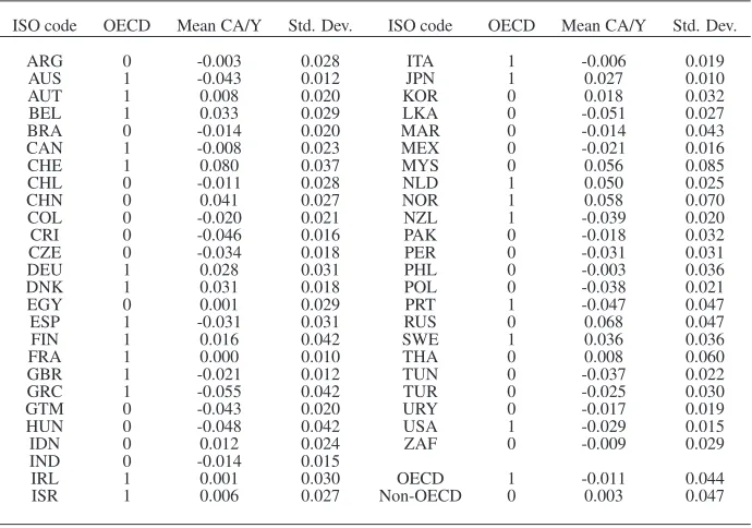
credit to GDP ratio which is taken from the World Bank. Table 2 lists the countries in the sample. There
are 22 rich OECD countries and 27 other countries. All these countries appear to experience large yearly
fluctuations in their CABs. The period covered by the sample is 1986-2013.
Table 3 provides a decomposition of the variation of these variables intheir between and within
com-ponents. Values of CABs are equally driven by average differences across countries and changes within
countries. In line with their classification, structural variables tend to be characterised by high ‘between’
variation and low ‘within’ variation whereas the opposite tends to hold true for cyclical and policy variables.
From an econometric perspective, low variation means difficult identification. It is therefore worthwhile to
consider the estimates obtained using both sources of variation.
[Table 1 about here.]
[Table 2 about here.]
[Table 3 about here.]
4.2
BMA results
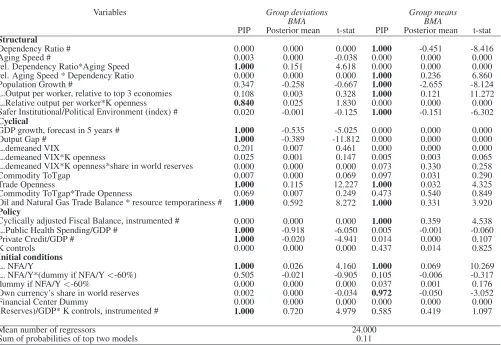
Results are presented in Tables 4-5. Using the full sample, we first assume slope homogeneity across
country groups and, in a second stage, we allow for slope heterogeneity between OECD and non-OECD
countries. At the bottom of each table, in addition to the average number of variables in each model, we
report the sum of the posterior model probabilities (PMPs) of the top two models. These probabilities
correspond to the proportion of draws taken from each model by the MC3 algorithm.
[Table 4 about here.]
[Table 5 about here.]
Table 4 shows that several variables included in the IMF-EBA model are not ‘BMA relevant’, with a
PIP close to zero. The set of relevant variables varies across data dimensions. Within estimates suggest
that changes in CABs are associated with changes in cyclical factors and policies while between estimates
indicate that differences in average CABs across countries tend to be related to structural factors. This
split agrees with economic intuition: transitory factors are associated with short-run movements in CABs
whereas slow-changing factors, such as demographic variables, are associated with durable differences in
CABs across countries. Variables deemed to be relevant have the expected sign (see Table 1).
Table 6 shows what would have happened if we had not decomposed the data into within and between
dimensions by combining BMA with a pooled estimator. A comparison of these results with those given in
Table 4 indicates that these estimates would have reflected the within estimates. In other words, the weight
given to the within estimator in the computation of the OLS estimator is extremely large in the context of
our empirical application. This implies that the pooled model, despite the absence of country fixed effects,
estimates in practice determinants of short-run changes in CABs.9
[Table 6 about here.]
The sum of the PMPs of the top two models is relatively low (0.11), highlighting that there is
con-siderable uncertainty about the right model. It is possible that this poor performance is the outcome of
slope heterogeneity across country groups. In Table 5, we thus allow for slope heterogeneity across country
groups by including interactions between every potential determinant of CABs and an OECD dummy
vari-able. Relative to the results of Table 4, The sum of the PMPs of the top two models is substantially higher
(from 0.11 to 0.20), indicating a reduction in model uncertainty, and we also observe a larger number of
relevant variables, e.g. fiscal balance or capital controls. OECD and non-OECD countries appear to have
many determinants in common. Nevertheless, slope homogeneity is occasionally rejected. For example,
changes in the fiscal balance has little effect on CABs in non-OECD countries but a large impact on the
CABs of OECD countries. Looking across data dimensions, there is again a ‘natural’ split between cyclical
and policy factors having more of a short-run effect and structural factors being associated with variations
in average CABs across countries. In light of the events surrounding the global financial crisis as well as
the Euro crisis, it is worth highlighting the negative impact on CABs of high growth expectations, a positive
output gap, a rising fiscal deficit, or excessive credit.
4.3
Discussion
Our results provide a contrasted perspective on the ‘effectiveness’ of the IMF-EBA model. With the use of a
pooled estimator (Table 6), we would conclude that a large number of variables put forward by the academic
literature and included in the IMF-EBA model are not relevant when alternative models are considered.
Once we allow for heterogenous responses across time horizons (Table 4) and country groups (Table 5),
this conclusion appears to be too harsh. The high model uncertainty highlighted by BMA is often the
outcome of assuming that the effects of a variable are the same across time or across space.
The interpretation of the ‘between’ estimates is difficult because we cannot rule out that unobserved
country heterogeneity generates an omitted variable bias. Two responses can be given to this issue.
First, a distinction ought to be made in the use of a model for ‘explaining’ and for ‘predicting’. Even in
absence of causal interpretation, the ‘between’ estimates remain useful topredict CABs values since they
directly capture the effects of observed variables, and indirectly, the effects of some omitted variables. They
complement the ‘within’ estimates, which have a more causal interpretation, and can therefore be used to
explainthe likely effects of factors such as government policies.
Second, the robustness of the ‘between’ estimates to the inclusion of country fixed effects can be
as-sessed to evaluate their causal nature. In the context of the OLS estimator, this is clearly impossible since
there would be perfect multicollinearity between the fixed effects and the group means. However, this is
possible, at least to a certain extent, using other modelling techniques such as ridge regression.
In the next two sections, we provide empirical applications to illustrate these two responses.
5
Prediction and normative evaluation of current account gaps
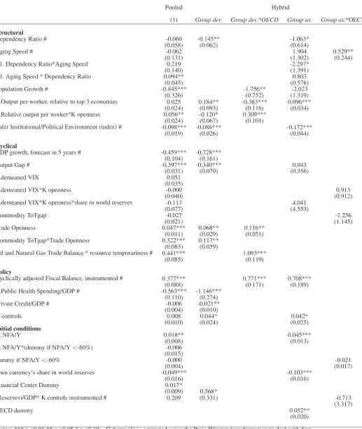
In this section, we explore the usefulness of our BMA exercise for the predictions and evaluations of current
account gaps. In Table 7, we estimate two models. The first model is a pooled model in which all variables
are included and homogeneity across time and space is assumed.10 The second model is our ‘best’ hybrid
10
model in the sense that we include all variables which are considered to be relevant in Table 5. Table 7
shows that the estimates between the two models tend to have the same sign but are often of a very different
order of magnitude. Interestingly, the estimates of the hybrid model tends to be close to those obtained
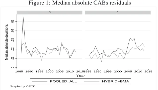
in Table 5. Figure 1 depicts the median absolute differences between observed and predicted values, by
year and country groups. Our hybrid model appears to perform better, in the sense that for most years, the
deviations are smaller than those of the pooled model.
[Table 7 about here.]
[Figure 1 about here.]
The IMF uses the predicted values generated by a pooled model to guide its normative evaluation of
CABs. A pooled model without country fixed effects or lagged dependent variable is estimated because the
IMF does not want to inflate the predictive power of their model by including proxies for unobservables.
The gaps between actual and predicted values are decomposed in an unexplained gap and a policy gap. The
latter, driven by variables which are expected to be under policy control in the short run (fiscal balances,
capital controls, social spending, reserve accumulation, and financial policies), corresponds to the estimated
coefficients times the difference between observed and desirable values of the policy variables. The two
stages of this approach can be refined by using a hybrid model rather than a pooled model while keeping
the spirit of the approach intact. The better fit of the hybrid model means smaller residuals to explain.
This implies that our knowledge of the determinants of CABs, or their surrogates if we believe that the
‘between’ estimates are tainted by an omitted variable bias, is better than what the predictions of the pooled
model would suggest. In addition, focusing on the ‘within’ estimates of policy variables allows for more
robust normative evaluations. These coefficients tend to capture short-run effects and can be given a more
causal interpretation since they are robust to country heterogeneity. Finally, the hybrid model obeys the
self-imposed modelling rules of the IMF which justify their use of a pooled model: no country fixed effects
or lagged dependent variable are included. Nevertheless, the coefficients on group deviations are still those
that we would obtain in a fixed effects model and, as discussed in Section 2, the ‘between’ estimates provide
some indications on long-run effects, as long as one is willing to assume that group means are uncorrelated
Our way of dealing with slope heterogeneity follows the common practice of economists and
practition-ers to decompose the world in OECD and non-OECD countries as these two groups are often expected to
have different behaviours.11 We could have gone one step further and allow for full slope heterogeneity.12
However, that would have created a tension between model flexibility and model operativeness. Assuming
that one wants to use the estimated model to do a normative evaluation similar in spirit to the one carried
out by the IMF in its EBA exercise, some cross-country constraints must be imposed to formulate ‘general’
policy recommendations. This preliminary normative analysis can then be adjusted using additional
infor-mation and the judgement of country experts. This is the iterative approach adopted by the IMF to obtain a
full assessment of external balances.
6
Dealing with unobserved country heterogeneity in a cross-sectional
setting
Our ‘between’ estimates may not truly capture the long-run responses of CABs as we cannot discount
the possibility of an omitted variable bias due to unobserved country heterogeneity. Hence, we wish to
investigate whether our cross-sectional results are robust to the presence of country-specific fixed effects.
This can be done through adding to the between regression in (2) a fixed effect for every country (i.e. adding
a dummy variable for each country). This sounds impossible to do since such a regression would have more
explanatory variables (N+K) than observations (N). Nevertheless, there is an increasing recognition that statistical methods exist to handle such cases.13
We now do BMA over a set of cross-sectional regressions where the set of explanatory variables contains
all those in Table 1 plusN fixed effects. Our BMA methods have to be slightly modified since the OLS
estimator and BIC cannot be applied when the number of regression coefficients is greater than the sample
size (nor can the g-prior, a common choice in BMA literature, be employed). To explain the necessary
modifications, note that BMA requires two things: i) a method for estimating regression coefficients in
11See for example the debate on global imbalances and the ‘savings glut’ initiated by Bernanke. The current account deficits of developed countries, notably the USA, are seen as the manifestation of the current account surpluses of emerging countries. See also Chinn and Prasad (2003) and Chinn and Ito (2007) for classical papers in the literature investigating current account determinants separately for industrial and developing countries.
12See Moral-Benito and Viani (2017) for such an application to the Spanish case.
13See for example this blog post aptly named ‘Fixed effects without panel data’:https://fxdiebold.blogspot.co.
each model; ii) weights for averaging across models. Consider first the estimation with a large number of
explanatory variables question. In the machine learning literature, there are several methods for dealing with
this issue (e.g. the Least absolute shrinkage and selection operator or LASSO). Many of these can be given
a Bayesian interpretation (Korobilis, 2013). In this paper, we apply the commonly used ridge regression
methods (see Hoerl and Kennard (1970)). The Bayesian interpretation of ridge regression methods is that
they amount to the use of a shrinkage prior. If β denotes all the regression coefficients (including the
coefficients on the country-specific dummy variables) and σ2 is the error variance, then ridge regression
amounts to using a N(0, τ×σ2I)prior where τ controls the strength of shrinkage (in this paper we set
τ = 10which is a relatively non-informative choice). This prior is natural conjugate and standard textbook results for Bayesian analysis of the regression model (e.g., chapter 3 in Koop (2003)), and can be used
to produce an estimate of any coefficient (i.e. its posterior mean) and the uncertainty associated with the
estimate (i.e. its posterior variance). Crucially, both of these can be obtained even when the number of
explanatory variables is greater than the number of observations.14 In addition, the marginal likelihood
exists in this case. The marginal likelihood is the standard Bayesian method of model comparison and,
asymptotically, its log converges to the BIC. Accordingly, it can be used to produce weights for the model
averaging.
[Table 8 about here.]
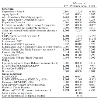
Table 8 presents the results of our BMA-ridge regression estimation. Given that ridge regression
in-volves standardisation of all variables before estimation, the estimated coefficients are not comparable to
those in previous Tables. For this reason, we focus on PIP and sign of the coefficients. It can be seen that
most PIPs are well below our threshold of relevance. This is certainly because we are asking a lot from
the data: we have 49 observations, 55 control variables, and 49 fixed effects. Nevertheless, the variables
with high PIP (above 0.50 here) tend be those with high PIP (above 0.75) in Table 5 and both tend to share
similar signs , e.g. political risk; fiscal balance; international indebtedness. Other variables, like ‘public
health spending’ now appears relevant to explain average differences in CABs across countries. Overall,
these results suggest that some of the ‘between’ estimates in Table 4 may reflect a causal relationship, albeit
with caveats.
7
Conclusion
Looking at the specific examination of the determinants of current account balances, this paper highlights
three features which are likely to be shared by many panel data applications: high model uncertainty,
pres-ence of slope heterogeneity, and potential divergpres-ence in short-run and long-run effects. The methodologies
deployed in this paper provide a response to these various issues. Their use ought to allow for more flexible
References
Aizenman, Joshua and Jinjarak, Yothin (2009) ‘Current account patterns and national real estate markets’,
Journal of Urban Economics, Vol. 66, pp. 75–89.
Avramov, Doron (2002) ‘Stock return predictability and model uncertainty’, Journal of Financial Eco-nomics, Vol. 64, pp. 423–258.
Baltagi, Badi H. and Griffin, James M. (1984) ‘Short and long run effects in pooled models’,International Economic Review, Vol. 25, pp. 631–645.
Bell, Andrew and Jones, Kelvyn (2015) ‘Explaining fixed effects: random effects modeling of time-series cross-sectional and panel data’,Political Science Research and Methods, Vol. 3, pp. 133–153.
Bernanke, Ben (2013) ‘The global saving glut and the current account deficit’,Technical report, Sandridge Lecture, Virginia association of economics, Richmond, Virginia, Federal Reserve Board.
Ca Zorzi, Michele, Chudik, Alexander, and Dieppe, Alistair (2012) ‘Thousands of models, one story: cur-rent account imbalances in the global economy’, Journal of International Money and Finance, Vol. 31, pp. 1319–1338.
Caballero, Ricardo J., Farhi, Emmanuel, and Gourinchas, Pierre-Olivier (2008) ‘An equilibrium model of global imbalances and low interest rates’,American Economic Review, Vol. 98, pp. 358–93.
Chinn, Menzie D., Eichengreen, Barry, and Ito, Hiro (2014) ‘A forensic analysis of global imbalances’,
Oxford Economic Papers, Vol. 66, pp. 465–490.
Chinn, Menzie D. and Ito, Hiro (2007) ‘Current account balances, financial development and institutions: assaying the world ‘saving glut’’,Journal of International Money and Finance, Vol. 26, pp. 546–569.
Chinn, Menzie D. and Prasad, Eswar S. (2003) ‘Medium-term determinants of current accounts in industrial and developing countries: an empirical exploration’, Journal of International Economics, Vol. 59, pp. 47–76.
Ciocyte, Ona and Rojas-Romagosa, Hugo (2015) ‘Literature survey on the theoretical explanations and empirical determinants of current account balances’, CPB Background Paper.
Clark, Tom S. and Linzer, Drew A. (2015) ‘Should I use fixed or random effects?’, Political Science Re-search and Methods, Vol. 3, pp. 399–408.
Cuaresma, Jes´us Crespo and Slacik, Tomas (2009) ‘On the determinants of currency crises: the role of model uncertainty’,Journal of Macroeconomics, Vol. 31, pp. 621–632.
Doppelhofer, Gernot, Miller, Ronald I., and Sala-i Martin, Xavier (2004) ‘Determinants of long-term growth: a Bayesian Averaging of Classical Estimates (BACE) approach’, American Economic Review, Vol. 94, pp. 813–835.
Doppelhofer, Gernot and Weeks, Melvyn (2009) ‘Jointness of growth determinants’, Journal of Applied Econometrics, Vol. 2, pp. 209–244.
Egger, Peter and Pfaffermayr, Michael (2002) ‘Long and Short Run Effects in Static Panel Models’, mimeo.
Eicher, Theo S., Papageorgiou, Chris, and Raftery, Adrian E. (2009) ‘Default priors and predictive per-formance in Bayesian model averaging, with application to growth determinants’, Journal of Applied Econometrics, Vol. 26, pp. 30–55.
Fernandez, Carmen, Ley, Eduardo, and Steel, Mark FJ. (2001) ‘Model uncertainty in cross-country growth regressions’,Journal of Applied Econometrics, Vol. 16, pp. 563–576.
Fogli, Alessandra and Perri, Fabrizio (2006) ‘The great moderation and the U.S. external imbalance’, Mon-etary and Economic Studies, Vol. 24, pp. 209–225.
Fratzscher, Marcel and Straub, Roland (2009) ‘Asset prices and current account fluctuations in G-7 economies’,IMF Staff Papers, Vol. 56, pp. 633–654.
Gourinchas, Pierre-Olivier and Rey, Helene (2014) ‘External adjustment, global imbalances, valuation ef-fects’, in Gita Gopinath, Elhanan Helpman, and Kenneth Rogoff eds. Handbook of International Eco-nomics: Elsevier, Chap. 10, pp. 585–645.
Greene, William (2008)Econometric Analysis: New Jersey: Peason Prentice Hall, 6th edition.
Hoerl, Arthur E. and Kennard, Robert W. (1970) ‘Ridge regression: biased estimation for nonorthogonal problems’,Technometrics, Vol. 12, pp. 55–67.
IMF (2013) ‘External balance assessment (EBA) methodology: technical background’,Technical report, International Monetary Fund.
Koop, Gary (2003)Bayesian Econometrics: Chichester: Wiley.
Koop, Gary and Potter, Simon (2004) ‘Forecasting in dynamic factor models using Bayesian model averag-ing’,The Econometrics Journal, Vol. 7, pp. 550–565.
Korobilis, Dimitris (2013) ‘Hierarchical shrinkage priors for dynamic regressions with many predictors’,
International Journal of Forecasting, Vol. 29, pp. 43–59.
Lane, Philip R. and Milesi-Ferretti, Gian Maria (2012) ‘External adjustment and the global crisis’,Journal of International Economics, Vol. 88, pp. 252–265.
Ley, Eduardo and Steel, Mark FJ. (2009) ‘On the effect of prior assumptions in Bayesian model averaging with applications to growth regression’,Journal of Applied Econometrics, Vol. 24, pp. 651–674.
Madigan, David, York, Jeremy, and Allard, Denis (1995) ‘Bayesian graphical models for discrete data’,
International Statistical Review, Vol. 63, pp. 215–232.
Sala-i Martin, Xavier (1997) ‘I Just Ran Two Million Regressions’,American Economic Review, Vol. 87, pp. 178–183.
Moral-Benito, Enrique (2012) ‘Determinants of economic growth: a Bayesian panel data approach’, The Review of Economics and Statistics, Vol. 94, pp. 566–579.
(2015) ‘Model averaging in economics: an overview’,Journal of Economic Surveys, Vol. 29, pp. 46–75.
Moral-Benito, Enrique and Roehn, Oliver (2016) ‘The impact of financial regulation on current account balances’,European Economic Review, Vol. 81, pp. 148–166.
Obstfeld, Maurice and Rogoff, Kenneth (1995) ‘The intertemporal approach to the current account’, in Gene M. Grossman and Kenneth Rogoff eds.Handbook of International Economics, Vol. 3 of Handbook of International Economics: Elsevier, Chap. 34, pp. 1731–1799.
Pesaran, Hashem M. and Smith, Ron (1995) ‘Estimating long-run relationships from dynamic heteroge-neous panels’,Journal of econometrics, Vol. 68, pp. 79–113.
Pirotte, Alain (1999) ‘Convergence of the static estimation toward the long run effects of dynamic panel data models’,Economics Letters, Vol. 63, pp. 151–158.
(2003) ‘Convergence of the static estimation toward the long run effects of dynamic panel data models: a labour demand illustration’,Applied Economics Letters, Vol. 10, pp. 843–847.
Pirotte, Alain and Mur, Jes´us (2017) ‘Neglected Dynamics and Spatial Dependence on Panel Data: Conse-quences for Convergence of the Usual Static Model Estimators’,Spatial Economic Analysis, Vol. 12, pp. 202–229.
Table 1: Potential determinants of current account balances
Determinants Definitions Expected impact Rationale
Structural
Dependency Ratio # Ratio of population aged over 65 divided by population between 30 and 64 years old.Also
interactedwith Aging Speed
- ; + ↓saving
Aging speed #Ω Projected change in the dependency ratio ratio 20 years out, relative to current level.Also
interactedwith Dependency Ratio
+; + ↑saving
Population Growth # Growth rate of the population - ↓saving
L.Output per worker, relative to top 3 economies
Ratio of PPP GDP to working age population relative to average of Germany, Japan, and U.S., demeaned.Also interactedwith K controls (see below)
-; + Capital flows from high
to low productivity countries Safer Institutional/Political Environment
(index) #
Average of 5 indicators from the International Country Risk Guide: socioeconomic conditions; investment profile; corruption; religious tensions; and democratic accountability. Higher values signify less risk
- ↑investment and↓saving
Cyclical
GDP growth, forecast in 5 years # Projections of the rate of real GDP growth 5 years ahead. Measured relative to the weighted world GDP averaged output gap
- ↑investment /↓saving
Output Gap # Estimated gap between current output and trend output - ↑investment and↓saving
L.demeaned VIXΩ VXO is an index of implied U.S. stock market volatility; it is interacted with K controls (see below). The latter interaction term isalso interactedwith the respective country’s share of its own currency share in world reserves (see below)
+; -; - Capital outflows; capital inflows due to flight to safety
Oil and Natural Gas Trade Balance * resource temporariness #
Positive net exports of oil and natural gas, as percentage of GDP, multiplied by a measure of resource exhaustion
+ ↑saving
Commodity ToTgapΩ* Trade Openness
Ω
Deviations from trend of a trade-weighted commodity terms of trade index.Also
interactedwith trade openness, measured as the ratio of exports and imports in goods and
services in GDP
+; + Better terms of trade
Changes in reserves, instrumented # Change in central bank foreign exchange reserves during the year scaled by nominal GDP, both in U.S. dollars, interacted with capital controls. Instrumented.
+ Reserve accumulation
Policy
Cyclically adjusted Fiscal Balance, instrumented #
Fiscal balance adjusted for the business cycle, instrumented + ↑saving if Ricardian equivalence does not hold
L.Public Health Spending/GDP # Proxy for social protection policy - Precautionary saving↓
Private Credit/GDP # Private credit to GDP ratio - Credit boom:↓saving /↑
investment
Capital controlsΩ Index on overall capital controls on the private sector (no controls to full controls). ?
Initial conditions
Lagged net foreign assets to GDP ratio Previous year’s value of the external net wealth to GDP ratio.Also interactedwith a dummy variable taking the value of one if the net foreign asset position is less than -60% of GDPΩ
+; - Higher investment revenue inflows
Own currency share in world reserves Share of the country’s own currency in total stock of world reserves - Exorbitant privilege Financial centre status Dummy variable that equals 1 for The Netherlands and for Switzerland throughout the
estimation period, and for Belgium also, but only through 2004
+ Ad-hoc.
Notes: ‘L.’: denotes one year lag. Variables followed by # are constructed relative to a (GDP-weighted) country sample average, in each year.Ω: variable not included on its own in the IMF-EBA model.↑: increase
2
Table 2: Countries in the sample
ISO code OECD Mean CA/Y Std. Dev. ISO code OECD Mean CA/Y Std. Dev.
ARG 0 -0.003 0.028 ITA 1 -0.006 0.019
AUS 1 -0.043 0.012 JPN 1 0.027 0.010
AUT 1 0.008 0.020 KOR 0 0.018 0.032
BEL 1 0.033 0.029 LKA 0 -0.051 0.027
BRA 0 -0.014 0.020 MAR 0 -0.014 0.043
CAN 1 -0.008 0.023 MEX 0 -0.021 0.016
CHE 1 0.080 0.037 MYS 0 0.056 0.085
CHL 0 -0.011 0.028 NLD 1 0.050 0.025
CHN 0 0.041 0.027 NOR 1 0.058 0.070
COL 0 -0.020 0.021 NZL 1 -0.039 0.020
CRI 0 -0.046 0.016 PAK 0 -0.018 0.032
CZE 0 -0.034 0.018 PER 0 -0.031 0.031
DEU 1 0.028 0.031 PHL 0 -0.003 0.036
DNK 1 0.031 0.018 POL 0 -0.038 0.021
EGY 0 0.001 0.029 PRT 1 -0.047 0.047
ESP 1 -0.031 0.031 RUS 0 0.068 0.047
FIN 1 0.016 0.042 SWE 1 0.036 0.036
FRA 1 0.000 0.010 THA 0 0.008 0.060
GBR 1 -0.021 0.012 TUN 0 -0.037 0.022
GRC 1 -0.055 0.042 TUR 0 -0.025 0.030
GTM 0 -0.043 0.020 URY 0 -0.017 0.019
HUN 0 -0.048 0.042 USA 1 -0.029 0.015
IDN 0 0.012 0.024 ZAF 0 -0.009 0.029
IND 0 -0.014 0.015
IRL 1 0.001 0.030 OECD 1 -0.011 0.044
Table 3: Decomposition of variables in between and within components
Variable Variation Mean Std. Dev. Min Max Variable Variation Mean Std. Dev. Min Max
Current account balance overall -0.005 0.046 -0.145 0.180 Commodity ToTgap overall -0.001 0.067 -0.334 0.412
between 0.034 -0.055 0.080 between 0.008 -0.030 0.025
within 0.032 -0.158 0.115 within 0.067 -0.349 0.387
Dependency Ratio # overall -0.040 0.094 -0.188 0.235 Trade Openness overall 0.324 0.180 0.041 1.101
between 0.092 -0.179 0.105 between 0.168 0.105 0.871
within 0.020 -0.158 0.125 within 0.069 -0.023 0.554
Aging Speed # overall -0.039 0.057 -0.184 0.185 Commodity ToTgap*Trade Openness overall -0.001 0.019 -0.115 0.118
between 0.050 -0.147 0.136 between 0.003 -0.010 0.008
within 0.027 -0.158 0.070 within 0.019 -0.119 0.110
rel. Dependency Ratio*Aging Speed overall -0.026 0.051 -0.178 0.213 Oil and Natural Gas Trade Balance * resource temporariness # overall 0.003 0.020 -0.005 0.215
between 0.043 -0.113 0.156 between 0.019 -0.004 0.118
within 0.026 -0.153 0.077 within 0.008 -0.062 0.099
rel. Aging Speed * Dependency Ratio overall -0.013 0.067 -0.247 0.257 Cyclically adjusted Fiscal Balance, instrumented # overall 0.005 0.023 -0.080 0.070
between 0.056 -0.168 0.095 between 0.021 -0.042 0.055
within 0.036 -0.351 0.150 within 0.011 -0.038 0.042
Population Growth # overall 0.002 0.007 -0.012 0.022 L.Public Health Spending/GDP # overall -0.012 0.023 -0.057 0.036
between 0.007 -0.009 0.017 between 0.022 -0.051 0.024
within 0.003 -0.009 0.012 within 0.006 -0.042 0.014
L.Output per worker, relative to top 3 economies overall 0.012 0.367 -0.526 1.013 Private Credit/GDP # overall -0.486 0.483 -1.298 0.988
between 0.369 -0.510 0.933 between 0.434 -1.061 0.704
within 0.046 -0.235 0.198 within 0.198 -1.478 0.508
L.Relative output per worker*K openness overall 0.065 0.300 -0.411 1.013 K controls overall 0.231 0.250 0.000 0.875
between 0.297 -0.372 0.857 between 0.216 0.000 0.757
within 0.055 -0.229 0.259 within 0.138 -0.207 0.736
Safer Institutional/Political Environment (index) # overall -0.063 0.145 -0.553 0.195 L. NFA/Y overall -0.221 0.352 -1.447 1.383
between 0.137 -0.414 0.130 between 0.310 -0.963 1.012
within 0.056 -0.257 0.123 within 0.169 -1.391 0.265
GDP growth, forecast in 5 years # overall 0.006 0.016 -0.026 0.060 L. NFA/Y*(dummy if NFA/Y ¡ -60%) overall -0.024 0.094 -0.847 0.000
between 0.015 -0.014 0.048 between 0.068 -0.363 0.000
within 0.008 -0.036 0.037 within 0.069 -0.832 0.193
Output Gap # overall 0.000 0.027 -0.143 0.120 Dummy if NFA/Y ¡ -60% overall 0.099 0.299 0.000 1.000
between 0.006 -0.013 0.022 between 0.222 0.000 1.000
within 0.026 -0.134 0.110 within 0.211 -0.781 1.063
L.demeaned VIX overall -0.003 0.065 -0.093 0.132 Own currency’s share in world reserves overall 0.049 0.122 0.000 0.715
between 0.006 -0.013 0.013 between 0.104 0.000 0.625
within 0.065 -0.110 0.140 within 0.057 -0.130 0.202
L.demeaned VIX*K openness overall -0.002 0.053 -0.093 0.132 Financial Center Dummy overall 0.053 0.224 0.000 1.000
between 0.005 -0.013 0.011 between 0.210 0.000 1.000
within 0.053 -0.107 0.141 within 0.062 -0.447 0.553
L.demeaned VIX*K openness*share in world reserves overall 0.000 0.009 -0.061 0.084 (Reserves)/GDP* K controls, instrumented # overall 0.001 0.009 -0.020 0.082
between 0.001 -0.001 0.002 between 0.008 -0.005 0.042
within 0.009 -0.059 0.085 within 0.006 -0.032 0.040
Notes: Each variable is decomposed into between (xi) and within (xi−xi+x; the global meanxis added back to make results comparable) components.
2
Table 4: Hybrid model: All countries
Variables Group deviations Group means
BMA BMA
PIP Posterior mean t-stat PIP Posterior mean t-stat
Structural
Dependency Ratio # 0.000 0.000 0.000 1.000 -0.451 -8.416
Aging Speed # 0.003 0.000 -0.038 0.000 0.000 0.000
rel. Dependency Ratio*Aging Speed 1.000 0.151 4.618 0.000 0.000 0.000
rel. Aging Speed * Dependency Ratio 0.000 0.000 0.000 1.000 0.236 6.860
Population Growth # 0.347 -0.258 -0.667 1.000 -2.655 -8.124
L.Output per worker, relative to top 3 economies 0.108 0.003 0.328 1.000 0.121 11.272
L.Relative output per worker*K openness 0.840 0.025 1.830 0.000 0.000 0.000
Safer Institutional/Political Environment (index) # 0.020 -0.001 -0.125 1.000 -0.151 -6.302
Cyclical
GDP growth, forecast in 5 years # 1.000 -0.535 -5.025 0.000 0.000 0.000
Output Gap # 1.000 -0.389 -11.812 0.000 0.000 0.000
L.demeaned VIX 0.201 0.007 0.461 0.000 0.000 0.000
L.demeaned VIX*K openness 0.025 0.001 0.147 0.005 0.003 0.065
L.demeaned VIX*K openness*share in world reserves 0.000 0.000 0.000 0.073 0.330 0.258
Commodity ToTgap 0.007 0.000 0.069 0.097 0.031 0.290
Trade Openness 1.000 0.115 12.227 1.000 0.032 4.325
Commodity ToTgap*Trade Openness 0.069 0.007 0.249 0.473 0.540 0.849
Oil and Natural Gas Trade Balance * resource temporariness # 1.000 0.592 8.272 1.000 0.331 3.920
Policy
Cyclically adjusted Fiscal Balance, instrumented # 0.000 0.000 0.000 1.000 0.359 4.538
L.Public Health Spending/GDP # 1.000 -0.918 -6.050 0.005 -0.001 -0.060
Private Credit/GDP # 1.000 -0.020 -4.941 0.014 0.000 0.107
K controls 0.000 0.000 0.000 0.437 0.014 0.825
Initial conditions
L. NFA/Y 1.000 0.026 4.160 1.000 0.069 10.269
L. NFA/Y*(dummy if NFA/Y<-60%) 0.505 -0.021 -0.905 0.105 -0.006 -0.317
dummy if NFA/Y<-60% 0.000 0.000 0.000 0.037 0.001 0.176
Own currency’s share in world reserves 0.002 0.000 -0.034 0.972 -0.050 -3.052
Financial Center Dummy 0.000 0.000 0.000 0.000 0.000 0.000
(Reserves)/GDP* K controls, instrumented # 1.000 0.720 4.979 0.585 0.419 1.097
Mean number of regressors 24.000
Sum of probabilities of top two models 0.11
Table 5: Accounting for slope heterogeneity
Group deviations Group deviations*OECD Group means Group means*OECD
Variables BMA BMA BMA BMA
PIP Posterior mean t-stat PIP Posterior mean t-stat PIP Posterior mean t-stat PIP Posterior mean t-stat
Structural
Dependency Ratio # 1.000 -0.223 -4.126 0.091 0.020 0.289 1.000 -2.146 -12.594 0.000 0.000 0.000
Aging Speed # 0.007 -0.001 -0.081 0.044 0.007 0.196 1.000 3.518 8.440 1.000 0.717 7.479
rel. Dependency Ratio*Aging Speed 0.000 0.000 0.000 0.028 0.003 0.155 1.000 -4.128 -9.492 0.000 0.000 0.000 rel. Aging Speed * Dependency Ratio 0.037 0.002 0.178 0.028 0.002 0.154 1.000 1.604 9.380 0.000 0.000 0.000
Population Growth # 0.000 0.000 0.000 0.998 -1.936 -4.453 1.000 -3.886 -9.454 0.000 0.000 0.000
L.Output per worker, relative to top 3 economies 1.000 0.138 4.053 1.000 -0.386 -5.601 1.000 0.225 12.901 0.000 0.000 0.000 L.Relative output per worker*K openness 0.874 -0.110 -1.984 1.000 0.335 3.574 0.000 0.000 0.000 0.000 0.000 0.000 Safer Institutional/Political Environment (index) # 0.990 -0.067 -4.260 0.019 -0.002 -0.126 1.000 -0.252 -9.034 0.000 0.000 0.000
Cyclical
GDP growth, forecast in 5 years # 1.000 -0.704 -7.063 0.000 0.000 0.000 0.013 0.005 0.099 0.000 0.000 0.000
Output Gap # 1.000 -0.324 -10.393 0.000 0.000 0.000 1.000 0.757 4.157 0.000 0.000 0.000
L.demeaned VIX 0.932 0.039 2.473 0.021 -0.001 -0.129 0.000 0.000 0.000 0.000 0.000 0.000
L.demeaned VIX*K openness 0.059 0.003 0.228 0.017 -0.001 -0.118 0.000 0.000 0.000 1.000 2.064 5.108
L.demeaned VIX*K openness*share in world reserves 0.000 0.000 0.000 0.000 0.000 0.000 1.000 17.289 5.137 0.000 0.000 0.000
Commodity ToTgap 0.020 0.000 -0.009 0.000 0.000 0.000 0.000 0.000 0.000 1.000 -2.626 -8.231
Trade Openness 1.000 0.108 10.451 0.981 0.084 3.136 0.008 0.000 0.069 0.358 0.012 0.678
Commodity ToTgap*Trade Openness 0.927 0.127 2.324 0.030 0.007 0.161 0.000 0.000 0.000 0.000 0.000 0.000
Oil and Natural Gas Trade Balance * resource temporariness # 0.000 0.000 0.000 1.000 1.016 10.493 0.000 0.000 0.000 0.000 0.000 0.000
Policy
Cyclically adjusted Fiscal Balance, instrumented # 0.000 0.000 0.000 1.000 0.689 5.535 1.000 0.813 10.795 0.000 0.000 0.000
L.Public Health Spending/GDP # 1.000 -0.978 -6.790 0.005 0.000 0.009 0.000 0.000 0.000 0.000 0.000 0.000
Private Credit/GDP # 0.994 -0.013 -3.376 0.000 0.000 0.000 0.000 0.000 0.000 0.000 0.000 0.000
K controls 0.980 0.049 3.016 0.011 0.000 -0.089 1.000 0.035 4.337 0.000 0.000 0.000
Initial conditions
L. NFA/Y 0.043 0.001 0.204 0.000 0.000 0.000 1.000 0.062 12.857 0.005 0.000 0.054
L. NFA/Y*(dummy if NFA/Y<-60%) 0.000 0.000 0.000 0.000 0.000 0.000 0.000 0.000 0.000 0.004 0.001 0.052
dummy if NFA/Y<-60% 0.000 0.000 0.000 0.008 0.000 -0.076 0.000 0.000 0.000 1.000 -0.053 -3.701
Own currency’s share in world reserves 0.291 -0.013 -0.597 0.651 -0.031 -1.177 1.000 -0.111 -8.940 0.000 0.000 0.000
Financial Center Dummy 0.000 0.000 0.000 0.000 0.000 0.000 0.000 0.000 0.000 0.000 0.000 0.000
(Reserves)/GDP* K controls, instrumented # 0.963 0.488 2.685 0.046 -0.048 -0.200 0.000 0.000 0.000 1.000 13.749 6.889
OECD dummy 1.000 0.065 7.985
Mean number of regressors 40.000
Sum of probabilities of top two models 0.200
Notes: PIP: Posterior Inclusion Probability. ‘BMA’: Bayesian Model Averaging.t-stat corresponds to posterior mean divided by posterior standard deviation. ‘L.’: denotes one
year lag. Variables followed by # are constructed relative to a (GDP-weighted) country sample average, in each year.
2
Table 6: Determinants of the current account: Pooled OLS estimator
All countries
PIP Posterior mean t-stat
Structural
Dependency Ratio # 0.161 -0.025 -0.388
Aging Speed # 0.040 0.004 0.182
rel. Dependency Ratio*Aging Speed 0.961 0.165 3.482
rel. Aging Speed * Dependency Ratio 0.070 0.006 0.258
Population Growth # 0.001 0.000 -0.020
L.Output per worker, relative to top 3 economies 0.002 0.000 -0.037
L.Relative output per worker*K openness 0.000 0.000 0.010
Safer Institutional/Political Environment (index) # 1.000 -0.057 -3.950
Cyclical
GDP growth, forecast in 5 years # 1.000 -0.631 -6.152
Output Gap # 1.000 -0.349 -11.585
L. demeaned VIX 0.725 0.027 1.408
L.demeaned VIX*K openness 0.237 0.010 0.523
L.demeaned VIX*K openness*share in world reserves 0.001 0.000 -0.015
Oil and Natural Gas Trade Balance * res temp # 1.000 0.553 5.593
Commodity ToTgap 0.014 0.000 0.107
Trade openness 1.000 0.110 9.290
Commodity ToTgap*Trade Openness 0.098 0.009 0.302
Policy
Cyclically adjusted Fiscal Balance, instrumented # 0.001 0.000 0.017
L.Public Health Spending/GDP # 1.000 -1.139 -7.934
Private Credit/GDP # 1.000 -0.028 -6.860
K controls 0.008 0.000 0.081
Initial conditions
L. NFA/GDP 1.000 0.047 7.793
L. NFA/GDP*(dummy if NFA/Y ¡ -60%) 1.000 -0.063 -4.365
Dummy if NFA/GDP ¡ -60% 0.000 0.000 -0.007
Own currency’s share in world reserves 0.002 0.000 -0.031
Financial Center Dummy 1.000 0.058 4.803
(Reserves)/GDP* K controls, instrumented # 0.999 0.595 4.493
Mean number of regressors 14.000
Sum of probabilities of top two models 0.70
Table 7: Predicting current account balances
Pooled Hybrid
(1) Group dev. Group dev.*OECD Group av. Group av.*OECD
Structural
Dependency Ratio # -0.060 -0.145** -1.063*
(0.058) (0.062) (0.614)
Aging Speed # -0.062 1.904 0.529**
(0.131) (1.302) (0.244)
rel. Dependency Ratio*Aging Speed 0.219 -2.297*
(0.140) (1.391)
rel. Aging Speed * Dependency Ratio 0.094** 0.803
(0.045) (0.576)
Population Growth # -0.845*** -1.756** -2.023
(0.326) (0.752) (1.319)
L.Output per worker, relative to top 3 economies 0.025 0.184** -0.383*** 0.096***
(0.024) (0.093) (0.116) (0.034)
L.Relative output per worker*K openness 0.056** -0.120* 0.309***
(0.024) (0.067) (0.101)
Safer Institutional/Political Environment (index) # -0.098*** -0.086*** -0.172***
(0.019) (0.026) (0.044)
Cyclical
GDP growth, forecast in 5 years # -0.459*** -0.728***
(0.104) (0.161)
Output Gap # -0.397*** -0.340*** 0.043
(0.031) (0.079) (0.356)
L.demeaned VIX 0.051
(0.035)
L.demeaned VIX*K openness -0.000 0.913
(0.040) (0.912)
L.demeaned VIX*K openness*share in world reserves -0.113 4.041
(0.077) (4.553)
Commodity ToTgap -0.027 -1.256
(0.021) (1.145)
Trade Openness 0.047*** 0.068** 0.116**
(0.011) (0.029) (0.051)
Commodity ToTgap*Trade Openness 0.322*** 0.117**
(0.083) (0.059)
Oil and Natural Gas Trade Balance * resource temporariness # 0.441*** 1.093***
(0.085) (0.119)
Policy
Cyclically adjusted Fiscal Balance, instrumented # 0.377*** 0.771*** 0.708***
(0.088) (0.171) (0.189)
L.Public Health Spending/GDP # -0.563*** -1.146***
(0.110) (0.274)
Private Credit/GDP # -0.006 -0.021**
(0.004) (0.010)
K controls 0.008 0.044* 0.042*
(0.010) (0.024) (0.025)
Initial conditions
L. NFA/Y 0.018** 0.045***
(0.008) (0.013)
L. NFA/Y*(dummy if NFA/Y<-60%) -0.006
(0.015)
dummy if NFA/Y<-60% -0.000 -0.021
(0.004) (0.017)
Own currency’s share in world reserves -0.049*** -0.103***
(0.016) (0.016)
Financial Center Dummy 0.017*
(0.009) 0.568*
(Reserves)/GDP* K controls instrumented # 0.209 (0.331) -0.713
(3.317)
OECD dummy 0.052**
(0.020)
Notes: *** p<0.01 ** p<0.05 * p<0.10. Column (1) is estimated using the Prais-Winsten transformation to deal with
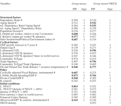
Table 8: Group means when controlling for unobserved country heterogeneity
Variables Group means Group means*OECD
PIP Sign PIP Sign
Structural factors
Dependency Ratio # 0.294 -1 0.310 1
Aging Speed # 0.312 -1 0.542 1
rel. Dependency Ratio*Aging Speed 0.364 -1 0.545 1
rel. Aging Speed * Dependency Ratio 0.296 -1 0.339 1
Population Growth # 0.234 -1 0.277 1
L.Output per worker, relative to top 3 economies 0.600 1 0.426 1
L.Relative output per worker*K openness 0.577 1 0.427 1
Safer Institutional/Political Environment (index) # 0.687 -1 0.319 1
Cyclical factors
GDP growth, forecast in 5 years # 0.365 1 0.343 -1
Output Gap # 0.139 -1 0.271 -1
L.demeaned VIX 0.236 1 0.596 1
L.demeaned VIX*K openness 0.210 -1 0.453 1
L.demeaned VIX*K openness*share in world reserves 0.347 1 0.346 1
Commodity ToTgap 0.474 1 0.414 -1
Trade Openness 0.497 1 0.796 1
Commodity ToTgap*Trade Openness 0.248 -1 0.405 1
Oil and Natural Gas Trade Balance * resource temporariness # 0.940 1 0.777 -1
Policy
Cyclically adjusted Fiscal Balance, instrumented # 0.607 1 0.275 1
L.Public Health Spending/GDP # 0.675 -1 0.766 1
Private Credit/GDP # 0.568 1 0.302 -1
K controls 0.343 1 0.251 -1
Initial conditions
L. NFA/Y 0.863 1 0.352 -1
L. NFA/Y*(dummy if NFA/Y<-60%) 0.261 1 0.273 -1
dummy if NFA/Y<-60% 0.321 -1 0.284 -1
Own currency’s share in world reserves 0.485 -1 0.482 -1
Financial Center Dummy 0.305 1 0.305 1
(Reserves)/GDP* K controls, instrumented # 0.543 1 0.339 1
OECD dummy 0.453 -1
Figure 1: Median absolute CABs residuals
0
.01
.02
.03
.04
.05
1985 1990 1995 2000 2005 2010 20151985 1990 1995 2000 2005 2010 2015
0 1
POOLED_ALL HYBRID−BMA
Median absolute deviations
Year