City, University of London Institutional Repository
Citation:
Kechagias-Stamatis, O. and Aouf, N. ORCID: 0000-0001-9291-4077 (2019). Fusing Deep Learning and Sparse Coding for SAR ATR. IEEE Transactions on Aerospace and Electronic Systems, 55(2), pp. 785-797. doi: 10.1109/TAES.2018.2864809This is the accepted version of the paper.
This version of the publication may differ from the final published
version.
Permanent repository link:
http://openaccess.city.ac.uk/id/eprint/23175/Link to published version:
http://dx.doi.org/10.1109/TAES.2018.2864809Copyright and reuse: City Research Online aims to make research
outputs of City, University of London available to a wider audience.
Copyright and Moral Rights remain with the author(s) and/or copyright
holders. URLs from City Research Online may be freely distributed and
linked to.
City Research Online: http://openaccess.city.ac.uk/ [email protected]
Abstract—We propose a multi-modal and multi-discipline data
fusion strategy appropriate for Automatic Target Recognition (ATR) on Synthetic Aperture Radar imagery. Our architecture fuses a proposed Clustered version of the AlexNet Convolutional Neural Network with Sparse Coding theory that is extended to facilitate an adaptive elastic net optimization concept. Evaluation on the MSTAR dataset yields the highest ATR performance reported yet which is 99.33% and 99.86% for the 3 and 10-class problems respectively.
Index Terms—Automatic Target Recognition, Convolutional
Neural Networks, Data Fusion, Sparse Coding, Synthetic Aperture Radar
I. INTRODUCTION
ODERN warfare requires high performing Automatic Target Recognition (ATR) algorithms to avoid collateral damage and fratricide. During the last decades, both industry and academia have made several ATR attempts in various data domains such as 2D Infrared [1], 3D Light Detection and Ranging (LIDAR) [2]–[4] and 2D Synthetic Aperture Radar [5]–[19] (SAR). Despite each data modality having its own
advantages, SAR imagery is appealing because it can be obtained under all-weather night-and-day conditions extending considerably the operational capabilities in the battlefield. Due to these advantages, SAR ATR has been attempted using various techniques.
Suggested methods include feature-based solutions where the SAR image is described by a set of robust attributes capable of achieving target classification under various nuisance factors. Feature-based solutions may rely on Krawtchouk moments [20] where features are derived from the discrete-defined Krawtchouk polynomials or on biologically inspired features. The latter can rely on episodic and semantic features [21] or sparse robust filters [22] that originate from the human cognition process. Other methods include binary operations [23], using the target’s scattering centers [15], [24] or the azimuth and range target profiles fusion [25].
Another type of SAR ATR algorithms uses a Stacked Autoencoder (SA) that extracts features from SAR imagery and inputs them to an SA type neural network. The latter is an
O. Kechagias-Stamatis and N. Aouf are with the Signals and Autonomy Group, Centre for Electronic Warfare Information and Cyber, Cranfield University, Defense Academy of the UK, Shrivenham, SN6 8LA, UK (e-mail: [email protected])
unsupervised learning structure used in neural networks that can convert the input data into abstract expressions utilizing a non-linear model. SA type SAR ATR suggests either exploiting Local Binary Features [18] or modifying the reconstruction error of the typical autoencoder scheme by adding an Euclidean distance restriction for the hidden layer features [17]. Other autoencoder based solutions are influenced by the human visual cortical system [26] or are combined with a Synergetic neural network concept [27].
Compressive Sensing (CS) has also been used for SAR ATR to recover the SAR signal that has been remapped from the originating domain into a domain where the signal is sparse using a non-adaptive linear projection. Signal recovery is achieved via an l1-norm optimization process. For example,
Multitask CS [28] exploits the statistical correlation among multiple target views to recover the target’s signature that is then used for target recognition under a compressive sensing scheme. Bayesian CS [14] relies on the scattering centers of the SAR image that are used as an input signal to the CS technique.
Sparse Representation Classification (SRC) or Sparse Coding (SC) type of solutions aim at recovering the SAR testing imagery out of a dictionary where the SAR training images are the dictionary’s base elements. SRC aims at identifying the sparsest representation of the testing imagery within the dictionary by employing an l1-norm optimization
scheme. The final classification decision mechanism matches the class that provides the smallest residual error. Joint SRC [29] for example, exploits three target views to increase the completeness of the target’s SAR signature and a mixed l0\l2 -norm. The reasoning of using multiple views is that these are highly correlated sharing the same response pattern within the dictionary and thus this conciseness can enhance the overall ATR performance. In [19] authors suggest the L1/2-NMF
technique that combines the l1/2-norm optimization to identify
the sparsest solution, with a Non-negative Matrix Factorization (NMF) scheme. The NMF features used as input to the SRC technique are the outcome of a NMF process that is applied on the SAR imagery. Dong et al. in [11] use the monogenic signal of a SAR image as an input to the SRC process. This signal comprises of the 2D SAR image signal and its Riesz transformed representation.
Deep Convolutional Neural Networks (CNNs) have also been suggested for SAR ATR. Literature proposes several CNN based solutions that use handcrafted CNNs [5], [8], [12], [13], [30] that are trained on SAR template images. Recently a
Fusing Deep Learning and Sparse Coding for
SAR ATR
Odysseas Kechagias-Stamatis and Nabil Aouf
Recurrent Neural Network is also suggested [31].
In the context of SAR ATR, SC and CNN based methods have individually shown theirs strengths by achieving quite high recognition rates. However, these techniques have not been fused yet such as to complement their strengths and afford an even higher recognition rate. Most important reasons to fuse SC and CNN based ATR are:
a. To extend the search space for the SAR ATR solution as SC and CNN ATR search for an ATR solution in different spaces. Indeed, SC ATR searches for linear projections between the target and the feature spaces while CNN ATR for non-linear projections. Hence, by fusing these two concepts, we essentially span a wider search area aiming a gaining higher ATR rates.
b. Combined classifiers can improve performance, as training a single classifier to work well for all test data is difficult. This multi-classifier strategy might not necessarily out-perform a single best performing classifier, but on average, it will perform better.
Driven by these reasons we fuse CNN and SC. Even though fusion in general, can be at a data, feature or decision level, in this paper we implement a decision level fusion. This is because the data modality for both contributing ATR modules, i.e. CNN and SC, is the SAR and therefore a data fusion scheme is not applicable. Additionally, despite feature-fusion could be an option, we neglected it as this would create an even larger feature encoding every SAR image, increasing the processing time needed to perform feature matching and neglecting it from military applications that require near-real time performance.
Additionally, state-of-the-art CNNs such as AlexNet [32], VGG [33], GoogleNet [34] and ResNet [35] have not been used in the context of SAR ATR. Driven by that, we suggest a novel architecture dubbed l1-2-CCNN that fuses an adaptive
1
l norm, l2norm SC scheme with a modified Clustered AlexNet CNN (CCNN) that uses a multi-class Support Vectors Machine (SVM) structure for final classification. The contributions of this paper can be summarized as:
a. In contrast to current SC based applications that use a fixed lpnorm, we propose a novel adaptive elastic net type
optimization that balances the advantages l1norm and 2
l normdepending on the characteristics of each scene SAR imagery. It is worth noting, that in contrast to current SC SAR ATR solutions, we neglect using the scattering centers of the SAR imagery in order to reduce the additional processing cost. b. We extend the usability of the AlexNet CNN from the visual domain to the SAR by introducing a hidden layer-clustering technique. This modification is combined with a multi-class SVM classification module that bridges the visual-SAR modality gap.
c. We innovatively fuse these two multi-discipline solutions under a decision level scheme that adaptively changes its fusion weights. Fusing these two techniques aims at expanding the search region of the SAR ATR solution and overcome the weaknesses of each of the two techniques.
The rest of the paper is organized in the following sections.
Section II introduces the proposed l1-2-CCNN architecture, while Section III evaluates our method on the MSTAR dataset. Finally, Section IV concludes the paper.
II. SARATRARCHITECTURE
The suggested architecture relies on a weighted SC, a clustered AlexNet variant and a decision level fusion scheme aiming at exploiting the advantages of all three techniques, each of which will be analyzed in the following paragraphs.
A. Sparse Coding
Sparse Representation or Coding aims at recovering a sparse representation x of a measured 1-dimensional signal
y
as a linear combination of a few atoms i.e. entries of a dictionary D [11], [29], [36], [37]:yDx with DM N ,MN Rank D, { }M (1) where xN1 is a coefficient vector whose non-zero entries determine the linear combination of the atoms in D that reconstruct measurement y. Ideally x should be K-sparse with K=1, i.e. all entries to be zero except from the one that associates y with the training sample within D.
Since MN, Eq. (1) is underdetermined and therefore has
infinite solutions. Determining the best solution
x
b is anoptimization problem that is ideally solved using the
0
l norm in order to identify the sparsest vector x0 out of the infinite solutions:
0 arg min
b
x x subject to Dxy (2) where || || : #{ :x 0 i xi 0}N , which counts the number of
non-zero entries in x. Solving Eq. (2) is NP-hard and therefore compressive sensing theory [38] suggests exploiting the sparse nature of the signal
y
(if it fulfills that prerequisite) and recovers the initial signal by solving the optimization problem:1
arg min
b
x x subject to Dxy (3) For 2-dimensional data such as SAR images Ia b , these are first remapped from the original a b image basis to a
e.g. noise.
Then the remapped images are converted into a m1
column vector with M c d [39] and are normalized to have a unit l2norm:
1
a b M sp
I I , M c d a b (4) Finally, the dictionary is defined as D[D D1, 2,...,Dj] where j is the number of training classes and each class is
defined as Do [Ispo_1,...,Ispo k_ ] m k,o j
with k the number of atoms/ entries per class j. Hence, we create an overcomplete dictionary M N
D with base elements the 1D SAR feature vectors of the corresponding SAR training images as created by Eq. (4). In contrast to current SC based SAR ATR methods [8], [11], [14], we do not create the 1D SAR feature vectors from pre-processed grayscale SAR images but from the raw grayscale SAR images. The advantage of using directly the grayscale SAR imagery is relaxing the complexity and thus reducing the processing burden of the proposed SC module without though sacrificing its SAR ATR performance (Section III). It is worth noting that the size of D has a major influence on the performance of the SC algorithm. Specifically, N
purely depends on the available training images, but the value of M, i.e. 1D feature vector length, even though fixed it is user-defined, meeting the constraints presented in Eq. (1). For this work, we examine several feature lengths such as to optimize the SC SAR ATR performance (Section III-B-1).
SC classification relies on the assumption that a new unknown test image '
I from class u that is converted into a 1D feature vector Isp' lies within the same subspace with the
training atoms of the same class. Thus Isp' can be represented
by Eq. (1) and solved with Eq. (3). It is reminded that the test SAR image is not input directly to Eq. (3) but we exploit its corresponding 1D feature vector Isp' that is produced
according to Eq. (4).
Driven by the underlying SAR imagery data structure, we generalize [40] and consider that an l1norm SC is effective for non-Gaussian type 1D SAR feature vectors, whereas
2
l norm for Gaussian type. Therefore, given a test SAR image, we first remap it according to Eq. (4) and then analyze its core structure to identify if it is a Gaussian or a non-Gaussian type. Specifically, we analyze the 1D SAR feature vector Isp' as a combination of a two-component Gaussian
Mixture Model (GMM) [41]:
2
' '
1
( sp) i sp i, i i
p I N I
(5)1 2 1
(6)
'
'
22
1
, exp
2 2
sp i sp i i
i i
I N I
(7)
where i, i and i are the mean, the variance and the
component weight of the ith GMM component of the 1D SAR
feature Isp' .
Then, we substitute Eq. (3) with an elastic net regularization technique [42] that is extended to use an adaptive coefficient estimator such as to optimize the regression problem depending on the GMM 1D SAR feature vector analysis :
2
2 1
arg min 1
b x
x a x a x subject to '
sp DxI (8) where a is the penalty factor that we adaptively define as:
1 max 0.5
a (9) such as a1 when max( ) i 0.5 and a0 when max( i) 1, with a very small constant (in our trials we use 105) and i the GMM component weight. We solve
Eq. (8) using the Least Angle Regression – Elastic Net (LARS-EN) [42], with a convergence threshold of 10-4 for the
cyclical coordinate descent [43] that is computed along the regularization path with 105 maximum iterations. Using the
LARS-EN solver implies the penalty factor to be in the range of (0,1].
It is important to note that in contrast to [40], our extension: a. Does not consider SC classification on 1D data that are affected by Gaussian and non-Gaussian noise. In our architecture, we solve Eq. (5) after analyzing the underlying structure of 2D SAR imagery and determine whether the core of this structure is governed by a Gaussian or a non-Gaussian distribution.
b. Does not involve a fixed value of the parameter α that is determined after a tuning process. Instead of that fixed approach, we adaptively estimate a for each 2D SAR target image that depends on a GMM based analysis of the target image. The advantage of this adaptive estimation is that it fully exploits the capabilities of the elastic net solution of Eq. (5) as it spans a to a range of possible values with a(0,1].
This methodology aims at determining whether a single dominant Gaussian distribution can or cannot describe the 1D feature Isp' of the SAR image
'
I , and accordingly adapt Eq.
(9) such as to optimize the elastic net given by Eq. (8). Fig.1 shows two extreme case examples where the 1D feature Isp' of
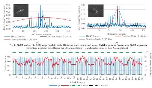
the SAR image I' (blue curve) is analyzed into a two-component GMM (black and red curve show the Gaussian distribution of each model). Depending on the contribution of each GMM, in Fig. 1(a) we show an example of a 1D feature vector that has two equally important Gaussian distributions and thus in Eq.(8) we input a0.922 ( max( ) 0.538), while in Fig. 1(b) an example of one dominant Gaussian distribution and hence in Eq.(8) we input a0.308 (
(a) (b)
[image:5.612.64.562.210.329.2]Fig. 1. GMM analysis of a SAR image (top left) in the 1D feature space showing (a) mutual GMM importance (b) dominant GMM importance (percentage highlights the influence per GMM distribution – GMMs scaled based on their % contribution)
Fig. 2. Dependency of penalty factor a with the dominant GMM distribution i
(dashed lines show pure 1
x for a1 and 2 2
x for a0 solution schemes) Fig. 2 shows the ivariation of the dominant Gaussian
component and the corresponding penalty factor a over a few example SAR images. From Fig. 2 it is evident that the contribution i of the dominant GMM varies based on the
SAR image reflectivity that affects the 1D feature vector Isp,
which in turn adaptively adjusts the penalty factor a (Eq. (9)) and ultimately influences the elastic net regularization of Eq. (8). Fig. 2 also shows the two extreme cases where the 1D SAR feature vector is a perfect balance of two GMMs i.e.
1 2 0.5
and thus a1 and therefore from Eq. (5) the SC ATR problem for that SAR image is solved purely based on l1norm. Fig. 2 also shows a hypothetical perfect imbalance of the two GMMs with 1 1 and 2 0 (or vice versa). In that case, a and from Eq. (5) the SC ATR problem for that SAR image is solved based on a l2norm scheme.
B. Clustered Convolutional Neural Networks
In the context of SAR ATR, literature suggests several CNN based solutions that rely on handcrafted CNNs [5], [7], [8], [12], [13]. A common feature of these CNN architectures is their relatively low depth that varies from six up to nine layers, opposing to the mainstream visual domain CNNs where layers are 23 for AlexNet [32], 16 or 19 for VGG [33] depending on the version, 22 for GoogleNet [34] and 152 for ResNet [35]. This is because visual images have a higher information content per pixel compared to the radar reflections
presented in a SAR image. Unarguably, current mainstream CNNs have an exceptional classification capability in the visual domain. A typical way to deviate these CNNs from the dataset these were trained on, is by exploiting the Transfer Learning technique [44]. Nevertheless, this technique is not always effective in steering the weights of the CNN towards a completely different data modality i.e. from visual to SAR imagery [45]. Additionally, the limited number of publicly available military SAR imagery imposes the SAR ATR CNNs to populate the training images either by creating artificial variants e.g. rotated versions of the existing templates or by sampling patches out of the image. Opposing to that, RGB images are widespread and thus the pre-trained CNNs [32]– [35], [46]–[48] for that domain can exploit a massively larger training set.
Driven by the advantages of the RGB pre-trained CNNs we propose a multi-discipline and multi-modal architecture that combines the concepts of CNN and Multiclass Support Vector Machine (M-SVM) classification [49]. The intention is to transfer the already proven classification capability of the AlexNet [32] from the RGB domain to the X-band SAR without using Transfer Learning [44]. This is because the combination of the completely different data modality between SAR and visual imagery along with the lack of SAR training samples imposes a huge constrain to steer the weights of these CNNs towards SAR data and thus offering a moderate classification performance [45].
AlexNet is a 23-layered network that encapsulates from an RGB image features that vary from low-level corners and blobs, in the initial hidden layers, up to high-level RGB
0 20 40 60 80 100
0 0.2 0.4 0.6 0.8 1
1 6 11 16 21 26 31 36 41 46 51 56 61 66 71 76 81 86 91 96
101 106 111 116 121 126 131 136 141 146 151 156 161 166 171 176 181 186 191 196 201
D
o
mi
na
nnt
G
M
M
φ
i
(%
)
P
ena
lt
y
f
ac
to
r
α
# SAR imagery
φi α l1-norm l2-norm^2
0.00 0.05 0.10 0.15 0.20 0.25
1 101 201 301 401 501
S
A
R
r
ef
le
cti
v
it
y
r
es
po
ns
e
SC feature elements
1D SC feature Gaussian Model 1 (84.6%)
Gaussian Model 2 (15.4%) 0.00
0.05 0.10 0.15 0.20 0.25 0.30 0.35
1 101 201 301 401 501
S
A
R
r
ef
le
cti
v
it
y
r
es
po
ns
e
SC feature elements
1D SC feature Gaussian Model 2 (53.8%)
oriented complex features in the last layers. Although AlexNet is powerful, it has been trained on the RGB images of ImageNet [50] that are completely different to SAR imagery. AlexNet is trained on RGB color bands while SAR images contain radar reflections. Therefore, directly applying AlexNet on SAR imagery is not an optimum solution. Hence, we group the 23 layers of AlexNet into nine clusters l of varying feature description capability, introducing the Clustered-AlexNet (C-Clustered-AlexNet) presented in Table I. Notation l refers to the cluster layer activated with l
1, 2,3, 4,5, 6, 7,8,9
. This means, for instance, l4 activates up to AlexNet’s clustered layer 4 while the remaining layers
5, 6, 7,8,9 are
discarded. C-AlexNet uses the same parameters (stride, padding and convolutional filter sizes) as in the original implementation [32].This specific clustering scheme is directly related to the position of the convolutional layers within AlexNet, which in turn are directly linked to the complexity of the features extracted from each cluster. That is, the deeper the convolutional layer, the more complex and data specific the detected features are. It should be noted that a fully connected layer is a convolutional layer that uses a kernel that has the size of the output of the previous hidden layer [51]. Therefore, the input layer of clusters six to eight is a fully connected rather than a convolutional layer.
Given a SAR image Ia b
, a b, Z and ( , ) {0,1,..., 255}
I s t with 1 s a and 1 t b, we initially remap I into a 3-D tensor to meet the input requirements of AlexNet:
1 ( ) ( ) ( )
I B I B I B I (10)
where B( ) is a bicubic interpolation process and || ( ) is a 3D concatenation of a single SAR image in order to replicate the RGB layers that AlexNet requires as an input.
OnceI1 is input to the C-AlexNet, it is transformed into a
3D tensor l H xW xDl l l
X which propagates through the hidden layers until it becomes the output Yl of the end-layer of
cluster l. Hence, X1
is the input to cluster l1, X2 is the output of cluster l1 and simultaneously the input to l2 etc. Notation Hl, Wl and Dl refer to the height, width and depth of the tensor at clustered layer l and an element belonging to
l
X has an index set of ( , ,l l l)
u v d with 0 l l u H
,
0 l l
v W
, 0 l l
d L
. Network activations are computed by forward propagating input I1 through the CNN architecture
up to the specified layer l. For the feedforward process we use a mini batch size of one i.e. one training instance per iteration to estimate the gradient of the loss function and estimate the response of the CNN network. The reasoning of choosing a mini batch size of one is to increase the accuracy of the response.
3D tensors Xl and Yl are stacks of 2D matrices that highlight features of various complexity in a response map type of representation. As the Xl tensor propagates within the CNN’s activated clusters and ultimately becomes tensor l
Y , the tensor’s size changes based on the size of the convolutional kernel of each layer. That is a kernel size of 11x11x3 for cluster 1, the height and width of which approximately halves for each subsequent convolution till cluster 3 and thereafter it stabilizes at a kernel size of 3x3
(height x width) . Tensors Xl and Yl can be regarded as a generalized scale-space theory [52] concept where the various scales are envisaged via the subsequent shrinking of the convolutional kernel size and the octaves via the kernel weights that are auto-adjusted by the CNN during the training stage. In computer vision, scale-space is an important theory for keypoint detection contributing to the robustness of pattern recognition algorithms. Therefore, by linking tensors Xl,Yl with scale-space theory, we highlight the importance of these tensors and validate their contribution in regards to pattern recognition tasks as examined in this paper.
As noted in Table I, the features that further propagate in our clustered SAR ATR architecture are the ones provided by the end-layer of each clustered layer l that may be a Rectified Linear Unit (ReLU) layer, a Max Pooling layer or a Fully Connected layer. Therefore, it is important to present the operating details of these layers.
1) ReLU
This layer increases the non-linearity of a CNN by applying an individual truncation process on every X u v dl( , ,l l l):
, , max 0, , ,
l l
u v d u v d
Y X (11)
where , ,
l u v d
Y is the output of the l cluster layer. The
advantages of ReLU against the classic tanh activation function are the reduction in training time [32] and incorporating a purely supervised training scheme avoiding the need of unsupervised pre-training [53].
2) Max Pooling
This operation substitutes a sub-region l s
X of size s x s, i.e. pooling size, of the tensor , ,
l u v d
X with its maximum value:
, , max
l l
u v d s
Y X (12)
TABLEI CLUSTERED ALEXNET LAYERS
C-AlexNet layer ID (l)
AlexNet
layer ID Operations involved 1 1-2-3-4-5 Image input – Convolution – ReLU –
Normalization – Max pooling 2 6-7-8-9 Convolution – ReLU – Normalization –
Max pooling 3 10-11 Convolution – ReLU 4 12-13 Convolution – ReLU
5 14-15-16 Convolution – ReLU – Max pooling 6 17-18 Fully connected - ReLU
7 19-20 Fully connected – ReLU 8 21 Fully connected
, ,
l u v d
Y will have a size of 1 /
l l
H H s, 1 /
l l
W W s and 1
l l D D .
3) Fully Connected
Through the fully connected layer, the l( , ,l l l) X u v d input
of size l l l
H W D is remapped to:
, ,
l l l
u v d
Y w X bias (13)
that has size o
l l l
H W D , where , ,
l u v d
w is the weight
parameter that the fully connected layer is aiming at tuning and o
l
H the height of Yl that is defined during the design of the convolutional neural network.
In the suggested architecture, the output tensor , ,
l u v d
Y of the
l cluster layer is remapped into a 1D-feature vector of length
l l l
u v d by undergoing a multi-feature fusion process. The latter is implemented via a multi-dimensional vectorization process defined as:
,
, , 1,1, ,1, 2,1, ,2, 1, , , , 1, 1
: [ ,..., , ,..., , ,..., ]
H W
T d u v d d H d d H d W d H W d u v
a a a a a a a
(14)
over dimension d which is then followed by a vectorization procedure:
, , , 1, 1
H W
l l
u v u v
y vec Y
(15)
where [1,..., ]d . The advantage of this multi-fusion process is encompassing both the feature responses and the topology of the features for the entire tensor depth.
4) Multi-class Support Vector Machines (M-SVM)
The yl feature produced from the C-AlexNet at layer l is then used to train a one-vs-all M-SVM classification scheme. Given j the number of classes, the gth class is trained with all
the examples in the gth class having positive labels and the remaining classes having negative labels. For h training
images, the data yl vs. target class Cl correlation is
1 1
( ,y Cll ),...(y Cllp, p),..., (y Clhl, h) with Clp {1,.., }j being the class of ylp. M-SVM performs multiple binary SVM
classification tasks and labels the yl feature belonging to the class that gains the highest response. For a detailed analysis on SVM classification, the reader is referred to [54].
C. Decision level fusion
The 1D vector xb obtained from Eq. (8) includes responses
from all the atoms within D regardless of the class these belong. Thus, we remap xb to facilitate a single normalized response per target class j given by:
max( )
p SC p
p
x r
x
(16)
with xpa subset of xb that includes only the responses of the
target class p, p j.
Similarly, the output Yl of the activated layer in the
clustered CNN module is converted into rpCNN so that each
target class has a single response:
CNN l p
r y
(17)
Then we normalize the response per target class obtained from the suggested SC and C-AlexNet modules, i.e. rpSCand
CNN p
r respectively, to make them comparable. Normalization
is done via the z-score technique and the SAR ATR decision-making function is based on a weighted winner takes it all concept that is given by:
arg max
CNN CNN SC SC p p p p
CNN SC p
p p r r r r
r r
(18)
where || ( ) is a 1D concatenation process, , ( )r r are the average and standard deviation of the corresponding SAR responses and is a regulating parameter:
1
1.25
template
I template
if S S E S
otherwise
(19)
with SI the target SAR image entropy, E a tuning parameter
while Stemplate and
Stemplate
the average and standard deviation of the entropy of the templates. The role of parameter is to tune finely the decision-making function of Eq. (19) depending on the deviation of the target’s SAR image disorder SI in comparison to the disorder of the templates.The value of λ=1.25 is determined experimentally.
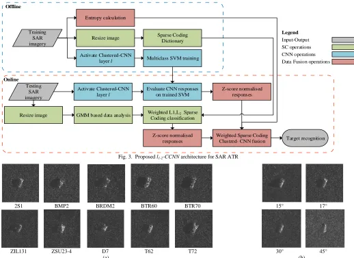
Our proposed Convolutional Neural Network and Sparse Coding data fusion architecture named l1-2-CCNN is presented in Fig. 3.
III. EXPERIMENTS
A. MSTAR dataset
We evaluate the performance of the proposed architecture on the MSTAR database [55], which includes the ground target classes presented in Fig. 4. Each class contains chips of 15° and 17° depression angles using an X-band SAR sensor,
Online Offline
Testing SAR imagery
Weighted L1,L2 Sparse
Coding classification
Z-score normalised responses
Z-score normalised responses Training
SAR imagery
Resize image Sparse Coding
Dictionary
Activate Clustered-CNN
layer l Multiclass SVM training
Evaluate CNN responses on trained SVM
Target recognition Resize image
Activate Clustered-CNN layer l
GMM based data analysis Entropy calculation
Weighted Sparse Coding Clustred- CNN fusion
Legend
[image:8.612.45.563.48.425.2]Input-Output SC operations CNN operations Data Fusion operations
Fig. 3. Proposed l1-2-CCNN architecture for SAR ATR
2S1 BMP2 BRDM2 BTR60 BTR70 15° 17°
ZIL131 ZSU23-4 D7 T62 T72 30° 45°
(a) (b)
Fig. 4. (a) 10 classes of the public MSTAR database at 17° depression angle (b) the 2S1 target at various depression angles while at same azimuth
TABLEII MSTARDATABASE
Target BMP2 BTR70 T72 BTR60 2S1 BRDM2 D7 T62 ZIL131 ZSU23/4 Sum ID 1 2 3 4 5 6 7 8 9 10 11 12 13 14
serial No 9563 9566 c21 c71 132 812 s7 k1 b01 e71 - a51 e12 d08
train 17° 233 232 233 233 232 231 228 256 299 298 299 299 299 299 SOC-1 2747
SOC-2 3671 test 15° 195 196 196 196 196 195 191 195 274 274 274 273 274 274 3203 test 30° - - - 288 287 - - - 288 863 test 45° - - - 288 287 - - - 303 878
B. 3-class problem
We use this experiment to fine-tune the free parameters of our architecture i.e. the modules of SC, C-Alexnet and decision level fusion. The target classes used are the BMP2, T72 and BTR70. For the former two we use all three variants namely the 9563, 9566 and c21, for the T72 the 132, 812 and s7 and for BTR70 the c71 which is the only one included in the dataset. Images captured at 17° depression angle are used as training and images at 15° for testing.
Specifically, our architecture is governed by the feature dimension m of the adaptive l1-2-norm SC (Eq. (8)), the layer l of the C-AlexNet that is activated (Table I) and the entropy boundary E (Eq. (19)) during the fusion stage. During tuning, we set as baseline values m=512, l=2 and E=3, and evaluate the 3-class ATR performance of the suggested technique by
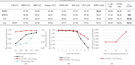
altering consecutively one of these three values. For the given baseline parameters, Table III highlights the performance of our architecture compared to current algorithms. It is evident that fusing the SC and CNN techniques under their suggested modified versions can outperform solutions that rely on a single method only. All trials are performed in MATLAB on an Intel i7 with 16GB RAM and an Nvidia Quadro K2200 GPU processor. MatConvNet [56] is used to implement AlexNet. The value of λ=1.25 in Eq. (19) does not affect the performance of the 3-class ATR problem.
1) Adaptive Lp-norm based SC optimization We create and evaluate a dictionary d1622
TABLEIII 3-CLASS ATR(%)
CM [57] BMO [23] SRF [22] Huang’s [21] DFSS [58] ASC [24] PCA [59] 2DPCA [60] l1-2-SC
only
CCNN only
l1-2
-CCNN
BMP2 - 97.28 94.89 94.38 91.65 97.27 97.44 99.15 94.90 98.30 98.5
BTR70 - 98.98 96.43 98.47 99.48 97.96 99.49 98.47 97.40 98.48 100
T72 - 97.78 96.91 96.91 96.04 97.53 95.92 98.45 96.90 99.14 99.50
Avg. 98.69 97.58 95.98 96.04 95.72 97.58 97.61 98.75 96.40 98.64 99.33
better the classification performance but the greater the processing time. Fig. 5 (a) shows that for the chosen feature length size of m=512, the total processing time for the fused SAR ATR solution we propose is 800ms. This is because by increasing the feature space dimension, the SC based encryption becomes more distinct but Eq. (8) requires more processing time to provide a solution.
2) C-AlexNet activation layer optimization
During this tuning phase, we vary the activating layer of the CCNN according to Table I. Fig. 5 (b) shows that the deeper the activated layer the more RGB specific the feature response becomes and harder to steer the CNN towards the SAR data domain. Thus the less capable the M-SVM is to linearly separate the three target classes in the activated feature space. Optimum performance for the suggested fused scheme is identified at l2 achieving 99.0% target recognition. 3) Decision level fusion optimization
We investigate how the decision level fusion regulating parameter E affects the overall performance of our proposed SAR ATR architecture. From Fig. 5 (c) it is evident that this parameter has a minor role to the overall performance but it can still affect it.
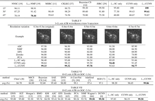
C. Assessment against large depression variation
For this trial, we use three similar targets, namely the 2S1, the BRDM2 and the ZSU 23-4. Images at 17° depression angle are used for training, while the 15°, and 30° and 45°for testing. Table IV shows that the suggested multi-discipline scheme affords a high performing ATR solution.
Depression variation involves a non-linear feature transformation and since our l1-2-norm solution seeks for linear
projections from the image space to the feature space the low performance of the SC module is anticipated [39].
D. Assessment against resolution variation
We challenge the robustness of the l1-2-CCNN to resolution variations from 0.3m×0.3m (original resolution), down to 0.7m×0.7m. Table V shows a target under these resolutions along with the performance of the suggested technique and the performance of current algorithms.
Table V shows that l1-2-CCNN outperforms all competitor solutions, while at the lowest resolution it still manages a 94.77% recognition rate. The robustness of l1-2-CCNN originates from the robustness of its individual modules i.e. the l1-2-SC and CCNN, which rely on the low-level abstract features extracted from the l2 layer of C-AlexNet and adaptive l-norm process of the l1-2-SC as described in Section
II-A.
E. 10-class ATR
Literature suggests various target configurations for the 10-class ATR problem, with commonly used the standard operation conditions 1 (SOC-1) and SOC-2. Although both are 10-class ATR subsets, their difference relates to the variants of BMP2 and T72 used. Specifically, SOC-1 for both training and testing includes only serial number 9563 for BMP2 and only serial number 132 for T72. SOC-2 uses all available serial numbers for both targets, for training and testing. Both SOC-1 and SOC-2 ATR evaluated based on the target’s class and not its serial number. For both target set configurations, the 17° depression angle is used for training and the 15° for testing.
Tables VI and VII compare the ATR performance of l1-2 -CCNN against current literature for the corresponding SOC-1
[image:9.612.40.574.65.323.2](a) (b) (c)
Fig. 5. Tuning parameters (a) SC feature space dimension (b) CCNN activation layer (c) E decision level fusion regulating value
0.00 0.50 1.00 1.50
0.80 0.85 0.90 0.95 1.00
64 128 256 512 1024
P
ro
ce
ss
in
g
ti
me
(
s)
R
ec
o
gni
ti
o
n
pe
rf
o
rma
nc
e
Feature space dimension
SC
CCNN - SC Fusion Processing time
0.50 0.60 0.70 0.80 0.90 1.00
1 2 3 4 5 6 7 8 9
R
ec
o
gni
ti
o
n
pe
rf
o
rma
nc
e
Activation layer l
CCNN
CCNN - SC Fusion
0.987 0.988 0.988 0.989 0.989 0.990 0.990
1σ 2σ 3σ
R
ec
o
gni
ti
o
n
pe
rf
o
rma
nc
e
Fusion regulating parameter E
TABLEIV
3-CLASS ATR WITH LARGE DEPRESSION VARIATION (%)
NNSC [19] L1/2-NMF [19] MSRC [11] CKLR2 [37] Bayesian CS
[14] JSRC [29] l1-2-SC only CCNN only l1-2-CCNN 15° 96.11 98.91 - 99.75 99.20 99.50 95.60 100 100
30° 87.25 91.42 98.49 98.29 89.60 91.80 77.30 99.43 99.61
45° 70.19 78.44 59.63 74.56 70.80 75.30 60.00 68.67 70.87
TABLEV
3-CLASS ATR WITH RESOLUTION VARIATION
Resolution variation 0.3m×0.3m (original) 0.4m×0.4m 0.5m×0.5m 0.6m×0.6m 0.7m×0.7m
Example
ASC 97.58 96.50 93.90 91.50 85.90
NMF 96.00 94.80 92.00 88.00 84.50
EFS 94.00 90.00 84.00 76.00 68.00
Zernike 96.00 92.00 86.00 82.00 74.00
PCA 95.00 94.00 91.00 87.00 84.00
l1-2-SC only 96.40 93.68 94.24 85.05 91.66
CCNN only 98.64 98.22 95.50 94.48 91.45
l1-2-CCNN 99.33 99.32 97.78 93.63 94.77
TABLEVI 10-CLASS ATR ON SOC-1(%) method Chen’s [8] MtCS
[28]
Bayesian CS [14]
SAE [18]
DNN [15]
A-ConvNet [5], [30]
AdaGrad
[7] SGD [7] l1-2-SC only CCNN only l1-2-CCNN
avg (%) 84.70 84.00 92.60 95.40 96.00 99.1 97.4 97.1 98.20 96.65 99.86
TABLEVII 10-CLASS ATR ON SOC-2(%) method DNN
[15] IGT [61]
Morgan’s [13]
BMO [23]
KM [20]
ASC [24]
EFS [62]
Zernike [63]
PCA [59]
NMF [19]
Wagner’s [64]
DCNN
[6] l1-2-SC only CCNN only l1-2-CCNN
avg (%) 95.00 95.00 92.30 95.74 84.58 95.41 94.10 93.46 90.24 93.76 99.50 99.50 97.83 96.19 99.50
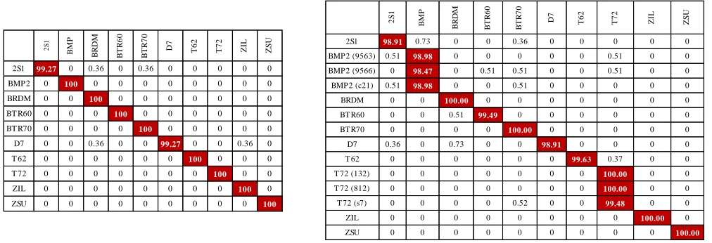
and SOC-2 MSTAR subsets. In both cases, the suggested l1-2 -CCNN achieves top ATR performance, which is 99.86% for SOC-1 and 99.50% for SOC-2. In addition, Fig. 6 shows the corresponding confusion matrix per SOC subset. For better readability, we present only the confusion matrix of l1-2 -CCNN.
F. 10-class ATR at various noise levels
In this trial, we evaluate the robustness of current proposals to various noise levels. Trials are on the SOC-1 subset and the noise simulation is consistent with [5], [11] i.e. we randomly select a percentage of pixels in the target scene and replace their values with samples generated from a uniform distribution. It should be noted that template images both for the SC and CNN module are the original ones. Table VIII presents the performance achieved for noise levels varying from 1% up to 15%. From Table VIII it is evident that the l1-2 -norm SC is extremely robust to noise levels due to its adaptive nature. Therefore, the l1-2-CCNN via its effective decision fusion process takes advantage of the high performing l1-2 -norm SC module and outperforms with a great margin current solutions on SOC-1 with additive noise.
G. Extending to other CNNs
From all trials it can be concluded that l1-2-SC and CCNN perform equally well for the 3-class and 10-class scenarios that do not have nuisance factors. The advantage of the fused
l1-2-CCNN is apparent because it preserves and even increases in quite a few cases, the robustness of CCNN in the depression angle variation scenario and of l1-2-SC in the additive noise scenarios.
Driven by the results achieved, we extend our layer-clustering strategy to VGG-16, GoogleNet and ResNet CNNs by utilizing their MatConvNet [56] implementations. As a reminder, similarly to AlexNet, all three CNNs are pre-trained on ImageNet [50]. The clustering methodology is similar to the one used for C-AlexNet, i.e. we cluster their layers so that the first layer of a cluster is a convolutional and the last layer is either a pooling or a ReLU layer. Based on the tuning process of Section III-B the optimum activation layer for the Clustered-VGG-16 (C-VGG-16) is l=2 that ends with the MaxPool_2 layer, while for the Clustered-GoogleNet (C-GoogleNet) is l=2 that ends with the Pool_2 layer. Finally, the Clustered-ResNet (C-ResNet) is l=3 that ends with the res2a_branch2b layer.
[image:10.612.48.570.67.410.2](a) (b)
Fig. 6. Confusion matrices (%) of l1-2-CCNN (a) SOC-1 (b) SOC-2 (rows are input classes and columns output classes)
TABLEVIII
10-CLASS SOC-1ATR WITH AT VARIOUS NOISE LEVELS
Gaussian noise level 0% 1% 5% 10% 15%
Example
A-ConvNet [5], [30] 99.13 91.76 88.52 75.84 54.68
l1-2-SC only 98.24 95.68 95.38 95.42 94.51
CCNN only 99.65 95.81 92.55 77.78 60.32
l1-2-CCNN 99.86 98.68 96.53 92.01 87.43
TABLEIX
PERFORMANCE ANALYSIS OF CCNNVARIANTS ON 10-CLASS SOC-1ATR
Method C-VGG C-GoogleNet C-AlexNet C-ResNet CCNN storage
(KB/template) 186.6 602.1 43.3 200.1 CCNN time
(ms/image) 6.35 14.65 17.50 45.9 CCNN only (%) 97.86 95.08 96.65 98.07
l1-2-CCNN (%) 99.58 99.53 99.86 99.57
TABLEX
3-CLASS ATR WITH VARIOUS CCNNVARIANTS (%)
Method BMP2 BTR70 T72
CCNN only (avg.)
l1-2-CCNN
C-VGG 22.83 10.71 95.38 52.19 94.32 C-GoogleNet 0.33 44.93 95.72 47.51 89.21 C-AlexNet 98.30 98.48 98.64 98.47 99.33
C-ResNet 10.23 81.12 92.29 61.21 91.71
We continue our trials by evaluating the ATR performance for the 3-class recognition case of Section III. Table X reveals that C-AlexNet outperforms C-VGG, C-GoogleNet and C-ResNet. This can be explained as:
a. Both C-VGG and C-AlexNet have the same internal layer construction up to the activated l=2 cluster but with different parameters i.e. convolutional filter and stride sizes. In fact, C-VGG has two 3x3 convolutional filters with stride one while C-AlexNet a 11x11 filter size with stride four and a 5x5 with stride two. By comparing the performance on the10-class SO1 and 3-class trials, we conclude that the filter size of C-VGG does not capture the intra-class spatial content of the target scenes as it is quite small. Even though the 3x3 convolutional kernel size is sufficient for RGB imagery because it has high-level features (and where VGG is trained for), our trials show that the SAR type data and the capability for intra-class ATR as in the 3-class ATR problem requires larger receptive filters to provide discriminative responses.
GoogleNet mainly uses inception modules rather than a standard deep network construction. The tuning process of C-GoogleNet provided as optimum cluster the l=2 ending with the Pool_2 layer and thus, a quite shallow part of the original GoogleNet is exploited even before the inception modules are applied. For the activated layer l=2, the two convolutional filters involve a 7x7 and a 3x3 kernel size and thus similarly to the C-VGG these are too small to encapsulate the intra-class SAR imagery information and bridge the original training with the testing modality gap i.e. visual vs. SAR imagery.
b. ResNet uses residual blocks. Each residual block encloses a convolutional filter of 3x3, which similarly to the C-VGG and C-GoogleNet, does not encapsulate efficiently the intra-class target variations.
By extending our architecture to facilitate the mainstream CNNs, we can draw the following conclusions. First, our concept is validated since in the SOC-1 ATR problem all CNNs have a similar performance. Second, the size of the convolutional filter plays an important role in the intra-class ATR performance. This is obvious from the 3-class scenario,
2
S1
B
M
P
B
R
D
M
B
T
R
6
0
B
T
R
7
0
D7 T62 T72 ZIL ZS
U
2S1 99.27 0 0.36 0 0.36 0 0 0 0 0
BMP2 0 100 0 0 0 0 0 0 0 0 BRDM 0 0 100 0 0 0 0 0 0 0 BT R60 0 0 0 100 0 0 0 0 0 0 BT R70 0 0 0 0 100 0 0 0 0 0
D7 0 0 0.36 0 0 99.27 0 0 0.36 0
T 62 0 0 0 0 0 0 100 0 0 0 T 72 0 0 0 0 0 0 0 100 0 0 ZIL 0 0 0 0 0 0 0 0 100 0 ZSU 0 0 0 0 0 0 0 0 0 100
2
S
1
B
M
P
B
R
D
M
B
T
R
6
0
B
T
R
7
0
D7 T62 T72 ZIL ZS
U
2S1 98.91 0.73 0 0 0.36 0 0 0 0 0
BMP2 (9563) 0.51 98.98 0 0 0 0 0 0.51 0 0 BMP2 (9566) 0 98.47 0 0.51 0.51 0 0 0.51 0 0 BMP2 (c21) 0.51 98.98 0 0 0.51 0 0 0 0 0
BRDM 0 0 100.00 0 0 0 0 0 0 0
BT R60 0 0 0.51 99.49 0 0 0 0 0 0
BT R70 0 0 0 0 100.00 0 0 0 0 0
D7 0.36 0 0.73 0 0 98.91 0 0 0 0
T 62 0 0 0 0 0 0 99.63 0.37 0 0
T 72 (132) 0 0 0 0 0 0 0 100.00 0 0 T 72 (812) 0 0 0 0 0 0 0 100.00 0 0 T 72 (s7) 0 0 0 0 0.52 0 0 99.48 0 0
ZIL 0 0 0 0 0 0 0 0 100.00 0
which highlights that the CNNs with a small filter size fail to classify correctly the target.
IV. CONCLUSION
Deep learning techniques for ATR of SAR imagery aim at extracting deep features that can uniquely describe a target within a SAR image. Instead of a single-discipline solution, we fuse a Convolutional Neural Network module with a Sparse Coding module. For the former, we extend the effectiveness of the AlexNet CNN to operate from the visual to the SAR domain by introducing a layer-clustering concept. In order to bridge the visual-SAR modality gap, the clustered-CNN is combined with a multi-class SVM classification scheme. The latter module (Sparse Coding), extends Sparse Coding theory to facilitate a proposed adaptive elastic net optimization concept that balances the advantages of
1
l norm and l2normoptimization based on the scene SAR imagery. Finally, the Clustered CNN and the adaptive Sparse Coding module are innovatively fused under a decision level scheme that adaptively alters the fusion weights based on the scene characteristics.
Experimental results on the MSTAR data set under various configurations such as the 10-class ATR problem with and without target variants, the 3-class ATR problem, and affected by several nuisance factors such as noise, large depression angle variation and resolution variation, illustrate the effectiveness of our suggested architecture against current ATR techniques. In fact, on the MSTAR dataset, our architecture yields the highest ATR performance reported yet in the literature, which is 99.33% and 99.86% for the 3 and 10-class problems respectively. Finally, we also demonstrate that among current CNNs used by the computer vision community, AlexNet has the unique characteristics to host this data modality extension.
REFERENCES
[1] Gray, G. J., Aouf, N., Richardson, M. A., Butters, B. and Walmsley, R., “An intelligent tracking algorithm for an imaging infrared anti-ship missile,” in Proc. SPIE 8543, Technologies for Optical Countermeasures IX, 2012, vol. 8543, p. 85430L–85430L. [2] Kechagias-Stamatis, O., Aouf, N., and Richardson, M. A., “3D
automatic target recognition for future LIDAR missiles,” IEEE Trans. Aerosp. Electron. Syst., vol. 52, no. 6, pp. 2662–2675, Dec. 2016.
[3] Kechagias-Stamatis, O., Aouf, N., “Evaluating 3D local descriptors for future LIDAR missiles with automatic target recognition capabilities,” Imaging Sci. J., vol. 65, no. 7, pp. 428–437, Aug. 2017.
[4] Kechagias-Stamatis, O., Aouf, N., Gray, G., Chermak, L., Richardson, M. A, and Oudyi, F., “Local feature based automatic target recognition for future 3D active homing seeker missiles,” Aerosp. Sci. Technol., vol. 73, pp. 309–317, Feb. 2018.
[5] Chen, S., Wang, H., Xu, F., and Jin, Y.-Q., “Target Classification Using the Deep Convolutional Networks for SAR Images,” IEEE Trans. Geosci. Remote Sens., vol. 54, no. 8, pp. 4806–4817, Aug. 2016.
[6] Zhong, Y. and Ettinger, G., “Enlightening Deep Neural Networks with Knowledge of Confounding Factors,” arXiv Prepr. arXiv1607.02397, pp. 1–10, 2016.
[7] Wilmanski, M., Kreucher, C. and Lauer, J., “Modern approaches in deep learning for SAR ATR,” in Proc. SPIE, 2016, vol. 9843, p. 98430N.
[8] Chen S. and Wang, H., “SAR target recognition based on deep learning,” in 2014 International Conference on Data Science and Advanced Analytics (DSAA), 2014, pp. 541–547.
[9] Paladini, R., Martorella, M. and Berizzi, F., “Classification of Man-Made Targets via Invariant Coherency-Matrix Eigenvector Decomposition of Polarimetric SAR/ISAR Images,” IEEE Trans. Geosci. Remote Sens., vol. 49, no. 8, pp. 3022–3034, Aug. 2011. [10] Perissin, D. and Ferretti, A., “Urban-Target Recognition by Means
of Repeated Spaceborne SAR Images,” IEEE Trans. Geosci. Remote Sens., vol. 45, no. 12, pp. 4043–4058, Dec. 2007.
[11] Dong, G., Wang, N. and Kuang, G., “Sparse Representation of Monogenic Signal: With Application to Target Recognition in SAR Images,” IEEE Signal Process. Lett., vol. 21, no. 8, pp. 952–956, Aug. 2014.
[12] Profeta, A., Rodriguez, A. and Clouse, H. S., “Convolutional neural networks for synthetic aperture radar classification,” in In SPIE Defense + Security International Society for Optics and Photonics, 2016, vol. 9843, p. 98430M.
[13] Morgan, D. A. E. “Deep convolutional neural networks for ATR from SAR imagery,” SPIE Def. + Secur., vol. 9475, p. 94750F, 2015.
[14] Zhang, X., Qin, J. and Li, G., “SAR target classification using Bayesian compressive sensing with scattering centers features,” Prog. Electromagn. Res., vol. 136, pp. 385–407, 2013.
[15] Doo, S., Smith, G., Baker, C., Cui, Z., Feng, J., Cao, Z., “Aspect invariant features for radar target recognition,” IET Radar, Sonar Navig., vol. 11, no. 4, pp. 597–604, Apr. 2017.
[16] Darymli, K., McGuire, P., W. Gill, E., Power, D. and Moloney, C., “ Holism-based features for target classification in focused and complex-valued synthetic aperture radar imagery,” IEEE Trans. Aerosp. Electron. Syst., vol. 52, no. 2, pp. 786–808, 2016.
[17] Deng, S., Du, L., Li, C., Ding, J. and Liu, H., “SAR Automatic Target Recognition Based on Euclidean Distance Restricted Autoencoder,” IEEE J. Sel. Top. Appl. Earth Obs. Remote Sens., vol. 10, no. 7, pp. 3323–3333, Jul. 2017.
[18] Kang, M., Ji, K., Leng, X., Xing, X. and Zou, H., “Synthetic Aperture Radar Target Recognition with Feature Fusion Based on a Stacked Autoencoder,” Sensors, vol. 17, no. 12, p. 192, Jan. 2017. [19] Cui, Z., Feng, J., Cao, Z., Ren, H. and Yang, J., “Target recognition
in synthetic aperture radar images via non-negative matrix factorisation,” IET Radar, Sonar Navig., vol. 9, no. 9, pp. 1376– 1385, Dec. 2015.
[20] Clemente, C., Pallotta, L., Gaglione, D., De Maio, A. and Soraghan, J. J., “Automatic Target Recognition of Military Vehicles With Krawtchouk Moments,” IEEE Trans. Aerosp. Electron. Syst., vol. 53, no. 1, pp. 493–500, Feb. 2017.
[21] Huang,, X., Nie, X., Wu, W., Qiao, H. and Zhang, B., “SAR target configuration recognition based on the biologically inspired model,” Neurocomputing, vol. 234, pp. 185–191, Apr. 2017.
[22] Yang, S., Wang, M., Long, H. and Liu, Z., “Sparse Robust Filters for scene classification of Synthetic Aperture Radar (SAR) images,” Neurocomputing, vol. 184, pp. 91–98, Apr. 2016.
[23] Ding, B., Wen, G., Ma, C. and Yang, X., “Target recognition in synthetic aperture radar images using binary morphological operations,” J. Appl. Remote Sens., vol. 10, no. 4, p. 046006, Oct. 2016.
[24] Ding, B., Wen, G., Zhong, J., Ma, C. and Yang, X., “A robust similarity measure for attributed scattering center sets with application to SAR ATR,” Neurocomputing, vol. 219, pp. 130–143, Jan. 2017.
[25] Gorovyi, I. M. and Sharapov, D. S., “Efficient object classification and recognition in SAR imagery,” in 2017 18th International Radar Symposium (IRS), 2017, pp. 1–7.
[26] Ni, J. C. and Xu, Y. L., “SAR automatic target recognition based on a visual cortical system,” in 2013 6th International Congress on Image and Signal Processing (CISP), 2013, vol. 2, pp. 778–782. [27] Sun,, Z., Xue, L. and Xu, Y., “Recognition of SAR target based on
multilayer auto-encoder and SNN,” Int. J. Innov. Comput. Inf. Control, vol. 9, no. 11, pp. 4331–4341, 2013.
[28] Liu, S., Zhan, R., Zhai, Q., Wang, W. and Zhang, J., “Multi-view radar target recognition based on multitask compressive sensing,” J. Electromagn. Waves Appl., vol. 29, no. 14, pp. 1917–1934, 2015. [29] Zhang, H., Nasrabadi, N. M., Zhang, Y. and Huang, T. S.,
2012.
[30] Wang, H., Chen, S., Xu, F. and Jin, Y.-Q., “Application of deep-learning algorithms to MSTAR data,” in 2015 IEEE International Geoscience and Remote Sensing Symposium (IGARSS), 2015, pp. 3743–3745.
[31] Yonel, B., Mason, E. and Yazici, B., “Deep Learning for Passive Synthetic Aperture Radar,” IEEE J. Sel. Top. Signal Process., vol. 12, no. 1, pp. 90–103, Feb. 2018.
[32] Krizhevsky, A., Sutskever, I. and Hinton, G., “Imagenet classification with deep convolutional neural networks,” in Advances in neural information processing systems, 2012, pp. 1097–1105.
[33] Simonyan, K. and Zisserman, A., “Very Deep Convolutional Networks for Large-Scale Image Recognition,” arXiv Prepr. arXiv1409.1556v6, pp. 1–14, Sep. 2014.
[34] Szegedy, C., Wei L., Yangqing J., Sermanet, P., Reed, S., Anguelov, D., Erhan, D., Vanhoucke, V., Rabinovich, A., “Going deeper with convolutions,” in 2015 IEEE Conference on Computer Vision and Pattern Recognition (CVPR), 2015, pp. 1–9.
[35] He, K., Zhang, X., Ren, S. and Sun, J., “Deep Residual Learning for Image Recognition,” in 2016 IEEE Conference on Computer Vision and Pattern Recognition (CVPR), 2016, pp. 770–778.
[36] Baraniuk, R., “Compressive Sensing [Lecture Notes],” IEEE Signal Process. Mag., vol. 24, no. 4, pp. 118–121, Jul. 2007.
[37] Dong, G. and Kuang, G., “Classification on the Monogenic Scale Space: Application to Target Recognition in SAR Image,” IEEE Trans. Image Process., vol. 24, no. 8, pp. 2527–2539, Aug. 2015. [38] Candes, E. J., Romberg, J. and Tao, T., “Robust uncertainty
principles: exact signal reconstruction from highly incomplete frequency information,” IEEE Trans. Inf. Theory, vol. 52, no. 2, pp. 489–509, Feb. 2006.
[39] Wright, J., Yang, A. Y., Ganesh, A., Sastry, S. S. and Ma, Y., “Robust Face Recognition via Sparse Representation,” IEEE Trans. Pattern Anal. Mach. Intell., vol. 31, no. 2, pp. 210–227, Feb. 2009. [40] Barazandeh, B., Bastani, K., Rafieisakhaei, M., Kim, S., Kong, Z.
and Nussbaum, M. A., “Robust Sparse Representation-Based Classification Using Online Sensor Data for Monitoring Manual Material Handling Tasks,” IEEE Trans. Autom. Sci. Eng., pp. 1–12, 2017.
[41] McLachlan, G. and Peel, D., Finite mixture models. New York, USA: John Wiley & Sons, 2004.
[42] Zou, H. and Hastie, T., “Regularization and variable selection via the elastic net,” J. R. Stat. Soc. Ser. B (Statistical Methodol., vol. 67, no. 2, pp. 301–320, Apr. 2005.
[43] Friedman, J., Hastie, T. and Tibshirani, R., “Regularization Paths for Generalized Linear Models via Coordinate Descent,” J. Stat. Softw., vol. 33, no. 1, 2010.
[44] Pan, S. J. and Yang, Q., “A Survey on Transfer Learning,” IEEE Trans. Knowl. Data Eng., vol. 22, no. 10, pp. 1345–1359, Oct. 2010. [45] Kang, C. and He, C., “SAR image classification based on the
multi-layer network and transfer learning of mid-level representations,” in 2016 IEEE International Geoscience and Remote Sensing Symposium (IGARSS), 2016, pp. 1146–1149.
[46] Marmanis, D., Datcu, M., Esch, T. and Stilla, U., “Deep Learning Earth Observation Classification Using ImageNet Pretrained Networks,” IEEE Geosci. Remote Sens. Lett., vol. 13, no. 1, pp. 105–109, Jan. 2016.
[47] Zha, S., Luisier, F., Andrews, W., Srivastava, N. and Salakhutdinov, R., “Exploiting Image-trained CNN Architectures for Unconstrained Video Classification,” in Procedings of the British Machine Vision Conference 2015, 2015, p. 60.1-60.13.
[48] Schwarz, M., Schulz, H. and Behnke, S., “RGB-D object recognition and pose estimation based on pre-trained convolutional neural network features,” in 2015 IEEE International Conference on Robotics and Automation (ICRA), 2015, no. May, pp. 1329–1335. [49] Mayoraz, E. and Alpaydin, E., “Support vector machines for
multi-class multi-classification,” in Engineering Applications of Bio-Inspired Artificial Neural Networks, 1999, pp. 833–842.
[50] “ImageNet.” [Online]. Available: http://www.image-net.org/. [Accessed: 15-Aug-2015].
[51] Wu, J., “Introduction to Convolutional Neural Networks,” Natl. Key Lab Nov. Softw. Technol., pp. 1–28, Nov. 2016.
[52] Lindeberg, T., “Scale-space theory: a basic tool for analyzing structures at different scales,” J. Appl. Stat., vol. 21, no. 1, pp. 225– 270, 1994.
[53] Glorot, X., Bordes, A. and Bengio, Y., “Deep Sparse Rectifier Neural Networks,” in Proceedings of the Fourteenth International Conference on Artificial Intelligence and Statistics, 2011, vol. 15, pp. 315–323.
[54] Wang, Z. and Xue, X., “Multi-Class Support Vector Machine,” in Support Vector Machines Applications, Cham: Springer International Publishing, 2014, pp. 23–48.
[55] Ross, T. D., Worrell, S. W., Velten, V. J., Mossing, J. C. and Bryant, M. L., “Standard SAR ATR Evaluation Experiments using the MSTAR Public Release Data Set,” in SPIE Conference on Algorithms for Synthetic Aperture Radar Imagery V, 1998, vol. 3370, pp. 566–573.
[56] Vedaldi, A. and Lenc, K., “MatConvNet,” in Proceedings of the 23rd ACM international conference on Multimedia - MM ’15, 2015, pp. 689–692.
[57] Bolourchi, P., Demirel, H. and Uysal, S., “Target recognition in SAR images using radial Chebyshev moments,” Signal, Image Video Process., vol. 11, no. 6, pp. 1033–1040, Sep. 2017.
[58] Liu, H. and Li, S., “Decision fusion of sparse representation and support vector machine for SAR image target recognition,” Neurocomputing, vol. 113, pp. 97–104, Aug. 2013.
[59] Zhang, R., Hong, J., Ming, F., Zhang, R., Hong, J. and Ming, F., “An improved PCA based features for SAR ATR,” in IET Conference Publications, 2009, no. 551 CP, pp. 313–313.
[60] Ding, B., Wen, G., Ye, F., Huang, X. and Yang, X., “Feature extraction based on 2D compressive sensing for SAR automatic target recognition,” in 2017 11th European Conference on Antennas and Propagation (EUCAP), 2017, pp. 1219–1223.
[61] Srinivas, U., Monga, V. and Raj, R. G., “SAR Automatic Target Recognition Using Discriminative Graphical Models,” IEEE Trans. Aerosp. Electron. Syst., vol. 50, no. 1, pp. 591–606, Jan. 2014. [62] Anagnostopoulos, G. C., “SVM-based target recognition from
synthetic aperture radar images using target region outline descriptors,” Nonlinear Anal. Theory, Methods Appl., vol. 71, no. 12, pp. 2934–2939, Dec. 2009.
[63] Rezai-rad, G. and Amoon, M., “Automatic target recognition of synthetic aperture radar (SAR) images based on optimal selection of Zernike moments features,” IET Comput. Vis., vol. 8, no. 2, pp. 77– 85, Apr. 2014.
[64] Wagner, S. A., “SAR ATR by a combination of convolutional neural network and support vector machines,” IEEE Trans. Aerosp. Electron. Syst., vol. 52, no. 6, pp. 2861–2872, Dec. 2016.
Odysseas Kechagias-Stamatis
received the MSc degree in Guided Weapon Systems and the PhD degree in 3D ATR for missile platforms from Cranfield University, U.K. in 2011 and 2017 respectively. His research interests include 2D/3D object recognition and tracking, data fusion and autonomy of systems.