Proceedings of the ASME 2019 38th International Conference on Ocean, Offshore and Arctic Engineering
OMAE2019 June 9-14, 2019, Glasgow, Scotland
OMAE2019-95578
A FLUID-STRUCTURE INTERACTION STUDY ON A PASSIVELY DEFORMED FISH FIN
Yang Luo, Qing Xiao1, Guangyu Shi, Zhiming Yuan
Department of Naval Architecture, Ocean and Marine Engineering, University of Strathclyde,
Glasgow, G4 0LZ, United Kingdom
Li Wen
School of Mechanical Engineering and Automation, Beihang University Beijing 100191, People’s Republic of China
1 Contact author: [email protected]
ABSTRACT
In this paper, the propulsive performance of a caudal peduncle-fin swimmer mimicking a bio-inspired robotic fish model is numerically studied using a fully coupled FSI solver. The model consists of a rigid peduncle and a flexible fin which pitches in a uniform flow. The flexible fin is modeled as a thin plate assigned with non-uniformly distributed stiffness. A finite volume method based in-house Navier-Stokes solver is used to solve the fluid equations while the fin deformation is resolved using a finite element code. The effect of the fin flexibility on the propulsive performance is investigated. The numerical results indicate that the compliance has a significant influence on the performance. Under the parameters studied in this paper, the medium flexible fin exhibits remarkable efficiency improvement as well as thrust augment, while the least flexible fin shows no obvious difference from the rigid one. However, for the most flexible fin, although the thrust production decreases sharply, the efficiency reaches the maximum value. It should be noted that by non-uniformly distributing the rigidity across the caudal fin, our model is able to replicate some fin deformation patterns observed in both the live fish and the experimental robotic fish.
INTRODUCTION
Morphologically, median fins and paired fins are two main categories of fish fins. Caudal fin, one type of the median fins, is mainly employed by fishes for thrust generation and maneuverability [1]. The previous studies on the fish swimming behavior for the autonomous underwater vehicle design are mainly focused on either rigid [2, 3] or flexible fins with uniformly distributed structural parameters [4, 5]. However, a
real fish fin is characterized as a composite structure composed of a membrane strengthened by fin rays [6]. Therefore, the simplified fin models with uniformly distributed stiffness may be unable to reflect the real fin’s propulsive performance and its bending pattern.
Some experiments and numerical simulations have been conducted to investigate the correlation between the inhomogeneous distribution of a caudal fin’s rigidity and its propulsion capabilities. For example, four passively-flexing fish-like foil models were designed by Lucas et al. to examine the effects of non-uniform stiffness on the swimming performance [7]. They found that the two foils with anterior regions of high stiffness and posterior regions of low stiffness outperform the foils with uniform distribution of flexibility in terms of self-propelled speeds and thrust production. The stiffness profiles of real fish were measured by Kancharala and Philen using digital image correlation (DIC) techniques [8]. With their experimental data, a chordwise varying stiffness robotic fin was fabricated to study the locomotion performance in a water tunnel. Their results indicated that the fins with varying stiffness generated larger thrusts and higher efficiency compared to the uniform ones. Numerically, Zhu and Bi developed a fully coupled FSI model to study the span-wise deformation on the dynamics of a ray-supported swaying caudal fin, and the performance enhancement through specific non-uniform distribution of rigidity on the fin was reported [9].
results by Esposito et al. [11] suggested that, on account of the existence of rays and thus the different stiffness of fin surface, the deformation of fin is not truly flat. In this work, inspired by the experiment conducted by Ren et al. [12], a model composed of a rigid peduncle and a flexible caudal fin with non-uniform flexibility is built to investigate the impact of three-dimensional deformation on fin’s propulsive performance through a fully coupled FSI numerical solver. Here, the homocercal fin is modeled as an elastic thin plate assigned with inhomogeneous rigidity, in which the rays-surrounding area is strengthened. The main objective of this study is to validate our newly developed FSI solver and then investigate how the compliance affects the propulsion performance of a caudal fin behind a locomotor peduncle.
1. Mathematical model and numerical approach In this section, the governing equations for the fluid and the solid are described. The fluid and structural domains are represented by f with the boundary f and s with s respectively. The fluid-structure interface i f s between the fluids and structures is the common boundary of the two domains.
1.1 Fluid solver
The governing equations of the flow around the caudal peduncle and fin can be expressed in the integral form as
0,f f
f c d f
d d
t
W
F F n (1)where n is the unit normal vector in outward direction,
W represents the conservative variable vector, the vector Fc
is the convective flux, and the diffusion flux is denoted by Fd. The in-house fluid solver solves the viscous, compressible flow using a cell-centered finite volume method based on a multi-block grid system. Using a structured methodology, the fluid domain f is divided into an array of hexahedral cells. The convective term is discretized by central JST scheme with an artificial dissipative term introduced by Jameson [13]. Green's theorem is applied to obtain the first order derivatives calculating the viscous flux tensors. For unsteady simulations, the dual-time stepping algorithm is used for time-integration [14].
Furthermore, the local time-stepping and multigrid method are implemented in the fluid solver to accelerate the convergence and implicit residual smoothing is applied to increase the stability of the solution. Parallelization is achieved via message passing interface (MPI) to enable large-scale computation.
1.2 Structural solver
The basic equation of the finite element method in the weak form of the balance of momentum can be written in the differential form as
2
2 2 ,
s s
D
D t
U P f (2)
where the acceleration of the material point is obtained by the second derivatives of the displacement vector U of the structure. Surface forces are modeled by the second Piola-Kirchoff stress tensor P and body forces of per unit mass such as gravity are represented byf. The solid density is denoted by
s .
The general governing equations of the solid dynamics, i.e. Eq. (2), are discretized using the finite element method. By applying the standard virtual work method, the linear algebraic equation system can be obtained by discretizing Eq. (2) in the whole solid domain as
22
,D Dt
K U M U F (3)
where
K is the global stiffness matrix,
M is the global matrix and
F is the global force vector respectively. By applying Newton's Second Law of Motion, the time domain is discretized using the -method with a second order accuracy here.In the present work, the implementation of finite element method solver is based on CalculiX written by Dhondt [15], in which a variety of element types including the brick element, the tetrahedral element and the wedge element are used to discretize the solid domain and define the shape functions. 1.3. Fluid-structure coupling
Considering the fluid solver [16] and CalculiX [15] are both highly specialized in its specific single-field physical solution and provide some advanced features, a partitioned coupling scheme is thus employed in order to keep the advantages from both solvers. In the present partitioned framework, an implicit scheme is designed to avoid the numerical instability that may be encountered when the mass ratio is low. In the present work, the fluid solver is integrated with CalculiX via preCICE (Precise Code Interaction Coupling Environment), a coupling library for partitioned multi-physics simulations [17].
2. The flexible caudal fin problem formulation
The current peduncle and caudal fin model is inspired by the experiment test conducted by Ren et al. [12], where a robotic fish tail mimicking the locomotion of the Bluegill Sunfish (Lepomis macrochrus) has been experimentally examined. In their experiment, the robot consists of a rigid
peduncle and a flexible caudal fin, and more details for the experimental setup can be found in [12].
Save the flow state intn
Grid deformation (spring-analogy method
+ TFI)
Solution of fluid equations (multistage Runge-Kutta
scheme)
Forces in the interface i
Forces interpolation (conservative mapping +
post-processing )
Solution of structural equations
in CalculiX yields Displacements
interpolation (consistent mapping +
post-processing: ) Convergence in
?
n t
No
Yes Update flow variables Increment totn1
1 0
n n k
Reload the flow state in tn
Sub-iteration loop
n k f
n k s n
k s
1
k k
[image:3.612.108.503.155.366.2]W
Fig. 1. Flow chart of the implicit FSI coupling in a partitioned approach.
Rotation motion
Rigid peduncle
Flexible caudal fin
O
80 mm
37.5
27.5
17.5
7.5
L=47 mm
10 mm
O
H=67 mm
W=5 mm t=0.8 mm
43.6 mm
O
(a) (b)
(c) (d)
A
[image:3.612.128.485.387.678.2]In this work, the geometry and dimensions of the peduncle and caudal fin is depicted in Fig. 2, where the geometrical data of the caudal fin is taken from the experiment [12] which is designed to replicate the shape of its real biological counterpart [22]. However, the peduncle is modified, as displayed in Fig. 2, to present a streamline fashion and a smooth transition from the peduncle to caudal fin, which mimics a real fish tail and also provides the ease for our CFD mesh generation.
The kinematics of the present model is described as follows. The peduncle combined with the caudal fin rotate harmonically around the z axis with the reference point O in a uniform flow in the positive x direction with a velocity of U . The time-dependent pitch motion of the model is described by
t msin 2
ft
, where m is the maximum amplitude and f denotes the oscillating frequency.
The dimensionless parameters are defined as : the Reynolds number ReUc/
, where c is the maximum chord length of the fin at angle 37.5 ; mass ratio m
st/
fc ; the reduced frequency f fc U/ ; the Poisson ratio the s; dimensionless stiffness KEI/
fU c2 3
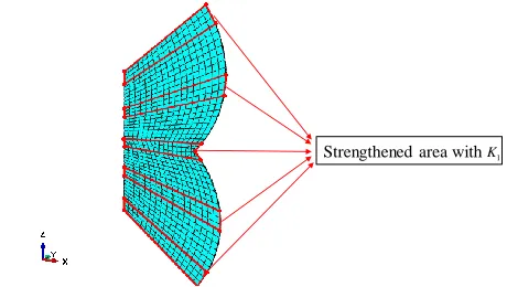
, where E is the Young’s modulus, It3/ 12 is the area moment of inertia of the cross section. [image:4.612.50.280.378.508.2]Strengthened area withK1
Fig. 3. The generated structural finite element mesh with locally strengthened area of the caudal fin.
2.1. Performance metrics
To evaluate the propulsion performance of the caudal fin, the instantaneous thrust and power coefficients are defined as
2
1 2
x T
f
F C
U S
(4)
3 , 1
2 P
f M C
U S
O (5)
where Fx is the total hydrodynamic forces on the caudal fin in x direction, S is the reference area, i.e. the area of the fin in xz surface, MO represents the z-component of the
reaction moment at point O. Meanwhile, the lateral force is defined as the hydrodynamic force in y direction
2 . 1
2 y L
f F C
U S
(6)
The propulsion efficiency is given by ,
T P C C
(7)
where CT and CP are the time-averaged values of CT and CP within one oscillating period.
2.2. Structural model of the caudal fin – the non-uniformity of flexible fins
In the experiment of Ren et al. [23], the fin consists of rigid rays and elastic membrane. The fin membrane is glued with the rays. Since the rays are relatively much smaller compared with the whole fin membrane surface, therefore, to simplify the modeling, the rays are not modeled explicitly in the present simulation. Nevertheless, considering the existence of the rigid rays, the stiffness of the caudal fin is strengthened locally surrounding the glued rays.
To consider the effect of the rays on the fin membrane, non-uniform distribution of Young’s modulus is assigned to the finite element model of the fin, as depicted in Fig. 3. The non-dimensional stiffness around the fin rays area K1 is larger than that K2 away from these areas, and K1rK r2, 1, where r is the stiffness ratio. By referencing the distribution of the material properties of a caudal fin inversely determined by Liu et al. [24] using a finite element analysis method, the stiffness ratio is selected as r2.
3. Validation and verification
3.1. Validation cases
The fluid solver used in the present work has been extensively validated in our previous work [16, 25-27]. Here the following three properly selected cases are used to validate the coupling of the fluid solver with CalculiX via preCICE. 3.1.1. Flow over a flexible cantilever behind a square cylinder
This problem consists of a fixed square bluff body with an elastic cantilever attaching in its wake [28-30]. Previous studies indicated that the flow separated from the leading edge of the square cylinder will induce a periodic oscillation of the flexible cantilever.
In this simulation, ReUd/
330 , the physical properties, i.e., mass ratio m
se/
fl 1.27
, non-dimensional bending stiffness K EI= /
fU l2 3
0.23 and Poisson's ratio s 0.35 are chosen to make the frequency of shedding vortex approximate the first Eigen-frequency of the cantilever, so that a remarkable oscillation can be observed. In the structural part, the left end of cantilever is set as fixed, and the movement of the whole cantilever is limited only in x and y direction.x y
U
d=0.01
l=0.04
e=0.0006
0.06 0.12
0.26
(a)
(b)
[image:5.612.321.580.172.315.2]Fig. 4. (a): Computational domain layout; and (b) generated mesh around the cantilever.
Fig. 5. Vertical tip displacement of the cantilever beam with different time step sizes.
Fig. 5 depicts the displacement of the free end of flexible beam in y direction with two dimensionless time step sizes, which are defined as t tU d/ . As seen, the displacement lies in a range of 0.85~1.30 cm, and the non-dimensional oscillation period T=TU d/ varies around 17.08
corresponding to the frequency f 1 / T 0.0585. It is very close to the theoretical Eigen-frequency of the flexible cantilever, which is 0.0591. Observed from previous published literature [28, 29, 31-33], the displacement amplitude lies between 0.8~1.4 cm, and T ranges between 15.80 and 17.44. Therefore, the current simulation results have good agreement with previous numerical solution.
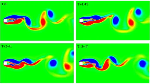
T+0 T+1/4T
[image:5.612.58.272.207.429.2]T+2/4T T+3/4T
Fig. 6. Evolution of vorticity in z direction within one oscillation period around the cantilever.
The vorticity contour in z direction within one oscillation period is represented in Fig. 6. The shedding of vortex can be observed clearly from the contour. During one oscillation cycle, two clockwise vortices form at the upper region while another two counter-clockwise appear at the lower region. It can be observed from the contour that the formed Von Karman vortex street behind the square bluff is dispersed by the oscillating elastic cantilever. Then it seems to be stretched along the downstream direction, but evolves to an independent round-similar shape away from the appendix.
3.1.2. The bending of a 3D flexible plate in uniform flow In this validation test, it involves a flexible plate which is bent while placed in cross flow. The original case derives from an experimental study on flow-induced reconfiguration of flexible aquatic vegetation conducted by Luhar and Nepf [34]. One of their experiment cases was then numerically simulated as a FSI validation by Tian et al. [35]. In their work, they quantitatively compared the results with experiment data in the presence of gravity and buoyancy and performed a series of simulations in the absence of them for a purpose of benchmarks studies. Here, the latter cases are chosen to validate our proposed multi-physics numerical suite.
The configuration of the elastic plate is depicted in Fig. 7. The plate is placed vertically in the cross flow with its bottom end clamp-mounted while the free end can deform under action of fluid forces. The parameters are all dimensionless: length
5
h b, thickness t0.2b, where b is the width, Reynolds nmber ReU h0 / =100 , mass ratio m*=
sb/
ft0.14,2 3 0
/ f 2.39
[image:5.612.61.273.464.613.2]The displacement of the plate center and the drag
coefficient, which is defined as 2
0
/ (0.5 )
d x f
C F
U bh , in the absence of gravity and buoyancy are compared in Table 1. It indicates that the present FSI simulation results match well with the counterparts in [35].0
U
h
b
[image:6.612.98.216.151.334.2]t
[image:6.612.343.554.165.306.2]Fig. 7. Layout of flow over an elastic plate.
Table 1. Comparison of drag coefficient and deformation in the absence of gravity and buoyancy when Re=100.
d
C Dx/b Dy/b
Tian el al. (2014) 1.02 2.34 0.67 Present study 1.06 2.31 0.678
3.1.3. The response of a flexible plate in a forced harmonic heave motion
This numerical validation case involves an experiment study conducted by Paraz et al. [36, 37]. It consists of a horizontal flexible plate which is made of polysiloxane. The plate has a rounded leading edge and a tapered trailing edge. The thickness of plate is 0.004m, chord length is 0.12m and span is 0.12m, giving an aspect ratio of 1. In their experiment, the leading edge was forced into a harmonic heave motion while the trailing edge was set free. The elastic plate deformed under the hydrodynamics forces. More detail about the experiment setup can be found in [37].
The simulation is carried out with a structured fluid domain which contains 57424 hexahedron cells along with 105 structural finite elements [15]. The response of the plate is characterized by the change of the relative displacement of the trailing edge with respect to that of the leading edge ATE/ALE and the phase difference between them. The response of the plate with varied forcing frequency is depicted in Fig. 8.
It can be found from Fig. 8 that the present simulation results match well with the counterparts in the experiment. A sharp peak is observed from the displacement curves of the trailing edge when the forcing frequency approaches the natural
frequency f0. At that point, the trailing edge displacement TE
[image:6.612.29.297.380.417.2]A is 1.5 times larger than theALE. This is the first resonance peak according to the analysis by Paraz et al. [37]. With the increase of forcing frequency, the phase shift experiences a continuous increase, indicating the strong interactions between fluid and structure with a large forcing frequency.
Fig. 8. The relative displacement of the trailing edge of the flexible plate with respect to that of the leading edge, ATE/ALE , and the corresponding phase shift as a function of the normalized frequency
0 /
f f for Re = 6000, ALE= 0.004 m and rigidity B=0.018 N m .
(a)
(b)
Fig. 9. Mode shape of the flexible plate when f /f0=1 obtained from experiment (a) [37] and current numerical simulation (b).
[image:6.612.338.549.381.518.2]3.2. Resolution verification
A resolution study is performed to assess the appropriate mesh and time-step resolution for ReUc/
2500 ,0.02
m , s 0.25, f 1, m 8 degree, and K2 5. Three grids are generated: a coarse grid with 2582214 nodes and minimum spacing of 1.6 10 3c in each direction, a medium grid with 3414712 nodes and minimum spacing of
4
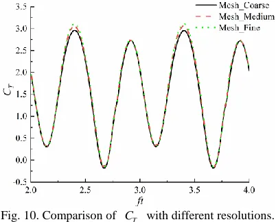
[image:7.612.314.582.94.178.2]1.2 10 c, and a fine grid with 5592570 nodes and minimum spacing of 8 10 4c. Furthermore, the non-dimensional time-step corresponding to the coarse grid is t f t 0.00909, the medium grid is t 0.00667 and the time step size for the fine one is t 0.00556. The results of CT when three different girds and time step sizes are used are shown in Fig. 10, and the mean coefficientsCT, CP as well as efficiency are compared in Table 2. Observed from the comparison, we find that the medium resolution setup is sufficient to simulate the flow filed around the caudal fin. Therefore, the medium grid with a time-step t 0.00667 is used for the following simulations.
[image:7.612.64.265.358.520.2]Fig. 10. Comparison of CT with different resolutions.
Table 2. CFD mesh and time-step resolution study results.
T
C CP
Mesh_Coarse 1.545 8.945 0.173 Mesh_Medium 1.599 9.131 0.175 Mesh_Fine 1.616 9.227 0.175
4. Results & Discussions
With the above code verifications, we applied the developed FSI tool to the rigid and flexible fins study as aforementioned. The Reynolds number under consideration is Re2500, the mass ratio is m 0.02 , the rotation angle
m
is 8 degree, the Poisson ratio s 0.25, and the reduced frequency is f 1. These parameters are chosen to match those in the experiment by Ren et al. [23].
Table 3. Summary of the time-mean thrust, lateral forces, power input coefficients and efficiency.
T
C CL CP
Rigid 0.5995 -0.0003 6.7056 0.0894
2 0.5
K 0.4321 0.3317 1.8952 0.2280
2 3
K 1.7784 0.9102 8.3562 0.2128
2 5
K 1.5992 0.7002 9.1314 0.1751
2 50
K 0.6944 0.00007 7.1918 0.0966
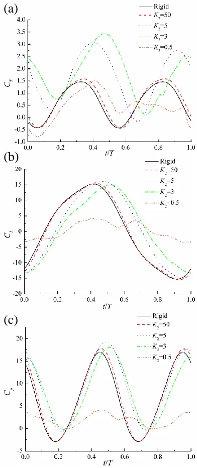
The predicted time-mean thrust, lateral forces, power input coefficients and efficiency of the caudal fin, when flexural stiffness is varied, are summarized in Table 3. As seen from the table, the flexibility of the fin has a significant effect on the propulsion performance of the caudal fin. The CT, CL, CP
and vary remarkably when the caudal fin is assigned with different flexural rigidities. Compared with a rigid caudal fin, mostly, a flexible one is able to generate larger thrust, especially when K2 3 the CT increase by 197%, almost three times as large as that of a rigid one. In fact, when the rigidity reaches a sufficient big level, the thrust and efficiency show no difference with the rigid counterpart. Oppositely, when the fin is too flexible, i.e., K2 0.5 , despite of the pronounced improvement of the efficiency, the thrust is very limited, which is even smaller than that of a rigid fin. These findings are consistent with the results in [38-42].
In terms of a power consumption, for flexible fins, it seems that the more thrust is generated, the more power input is needed. The only exceptional case is K2 3, in which the largest thrust is produced, while its needed power expenditure is not the most. In general, for compliant fins, the increase of power input is not as remarkable as the improvement of thrust, so the overall efficiency is enhanced compared with a rigid fin. The time history of the thrust coefficient, the normalized lateral forces and power input coefficient are demonstrated in Fig. 11. To facilitate description, these cases are categorized into three types: the least flexible cases (rigid find and the fin with K2 50), the medium flexible cases (the fin with K2 3 and K2 5) and a highly flexible case (the fin with K2 0.5), according to their propulsion capability shown in Table 3.
As observed in Fig. 11(a), within one oscillation period, apart from the highly flexible case, the other two patterns both present two thrust peaks, though with different amplitudes. It is noted that the two crests of the rigid fin and the fin with
2=50
[image:7.612.29.297.546.596.2]maneuverability for the fish. In comparison, the CT curves of the least and highly flexible cases have lower peaks and flatter troughs, especially that of the fin with the smallest rigidity only fluctuates in a small range of amplitude in the second half flapping.
(a)
(b)
[image:8.612.69.265.150.616.2](c)
Fig. 11. Instantaneous thrust coefficient CT, lateral forces coefficient L
C and power input coefficient CP over one flapping period when 2
K is 0.5 (orange dash dot dot line), 3 (green dash dot line), 5 (blue dot line), 50 (red dash line) and the fin is rigid (black solid line).
Nevertheless, all the power input coefficient curves almost have a similar fashion except for that of the highly flexible fin. The CP curve of the most compliant fin have a much smaller
[image:8.612.346.555.158.306.2]amplitude throughout most of the flapping cycle, so despite the least mean thrust output, it attains the most efficient propulsion. Interestingly, by comparing Fig. 11(a) with Fig. 11(c), it can be observed that the instantaneous thrust generation and power input almost reach the peaks at the same time, i.e. around the middle of the flapping period, when K2 3.
Fig. 12. Trajectory of the point A over one flapping period when K2 is 0.5 (orange dash dot dot line), 3 (green dash dot line), 5 (blue dot
line), 50 (red dash line) and the fin is rigid (black solid line).
(a)
(b)
Fig. 13. Images from high-speed video of a live Bluegill fish in flat motion adopted from [11] (a) and that of the current caudal
peduncle-fin model (b) when K23 at time t+T.
Like the power input plot, the lateral forces of the highly flexible fin presents a totally different fashion as others, of which all have clear peaks emerging around 2/5~3/5 T. However, owing to a continuous low lateral forces generated by the highly flexible fin, it may benefit to a straight-line cruising swimming for a fish.
[image:8.612.360.537.354.518.2]thus their motion curves are parabolas. However, when the fin is more compliant, their trajectories become figure-eight shapes, which is reminiscent of the typical orbital trajectories of the vortex induced vibration (VIV) of a cylinder [43].
(a)
[image:9.612.79.257.133.340.2](b)
Fig. 14. The fin deformation patterns of the trailing edge of the fin with K23 (a), and posterior view of the robotic caudal fin in [44]
(b).
By comparing the images obtained from a high-speed camera from the experiment of Esposito et al. [11] and that of the present caudal fin model in Fig. 13, it can be found that they appear similar curvatures of the trailing edges. Owing to the reinforcement of the rigidity of the middle part of the caudal fin, it seems that the middle trailing edge have a phase delay compared with the dorsal and ventral parts, which is observed in the bending of fish caudal fin. This distinguishes the current simulation from most of existing numerical studies in which only a uniformly distributed stiffness is considered. It can be further observed clearly in Fig. 14, in which the curvature patterns of the trailing edge of the caudal fin in yz plane during one flapping period is depicted, to demonstrate a highly three-dimensional deformation. Moreover, even though, no active control of fin rays is imposed, a similar bending form to that of the robotic fin in the experiment [44] is observed. As a matter of fact, according to the results of the simulations by Zhu and Bi [9], more complex deformation patterns of caudal fins, e.g. W-shape, can be achieved by imposing specific distribution of the flexibility of fish rays (fin).
The wake flow of the rigid and flexible fins (K2 3) are presented in Fig. 15. Two tip vortices shed from the dorsal- and ventral-most of the trailing edge of the caudal fin are formed parallel and alternatively. They have opposite rotation directions with one in counterclockwise while the other clockwise, and their vortices are approximately equal. These results match with those obtained in the experiments [11] and
[23] using digital particle image velocimetry (DPIV) techniques, and to our knowledge, no similar vorticity patters are reported by previous FSI studies. In comparison, the intensity of the vortices behind the flexible fin outperforms that of a rigid counterpart and it also has farther influence zone in the wake. As a result, the flexible fin generates larger thrust than the rigid one. This may explain the thrust augment shown in Fig. 11 (a).
(a)
(b)
Fig. 15. The wake flows contoured in Y vorticity of the flexible fin with K23 (a) and the rigid fin in the xz plane of y=0.005 m at the
time t+T.
(a)
[image:9.612.363.533.164.415.2](b)
[image:9.612.364.537.464.667.2]The wake structures of the flexible fin with K2 3 and the rigid fin are depicted in Fig. 16. It can be observed that different wake patterns are presented between the two cases. Two trains of vortex rings are formed in their wake with distinct shapes. In comparison, the geometry of the wake of the deformable fin is more complex with some small vortices attached around the main vortex rings, while the wake of the rigid one is more regular. In addition, the wake structure of the rigid fin appear to be compressed in the spanwise direction compared with that of the flexible counterpart, which appears to expand in both dorsal and ventral directions and also along the further wake instead. This is consistent with the Y vorticity contour in Fig. 15 indicating that a three-dimensional deformation of the fin makes the wake pattern more complex. 5. Conclusions
In this work, a fully coupled FSI solver is proposed by combining our in-house fluid solver with a finite element method based code CalculiX via preCICE. Three FSI validations are conducted to verify this multi-physics solver. Beyond that, the developed tool is applied to study the propulsive performance of a caudal peduncle-fin swimmer with non-uniform distribution of stiffness. It is found that the compliance of the caudal fin has a significant impact on its propulsion performance. With the parameters selected in this paper, the flexible fins outperform the rigid counterparts in terms of thrust generation and/or propulsion efficiency. The degree to which is profoundly affected by the assigned inflexibility. Interestingly, via apposing inhomogeneous distribution of the rigidity of fins, some curvature patterns of caudal fin, observed from live fish and bio-inspired experimental robotic fish, are presented from our simulation results.
It must be noted that due to the simplified model for the distribution of caudal fin rigidity, the effect of more complex situation, such as the variations of the flexibility in spanwise direction of fin, is not investigated. In addition, the chordwise distribution of flexural rigidity of a real fish fin is non-uniform while we assumed it is uniform in this study. Obviously, more deep investigations are needed to elucidate the above mentioned effects for a better understanding in this problem .
Acknowledgment
This work used the Cirrus UK National Tier-2 HPC Service at EPCC (http://www.cirrus.ac.uk) funded by the University of Edinburgh and EPSRC (EP/P020267/1). The first author would like to thank Dr. Benjamin Uekermann in Technical University of Munich for his kind suggestions about the coding works of the FSI coupling, and also thank China Scholarship Council (CSC) for the financial support during his study in the UK.
References
[1] R. Salazar, V. Fuentes, A. Abdelkefi, Classification of biological and bioinspired aquatic systems: A review, Ocean Engineering, 148 (2018) 75-114.
[2] G.S. Triantafyllou, M. Triantafyllou, M. Grosenbaugh, Optimal thrust development in oscillating foils with application to fish propulsion, Journal of Fluids and Structures, 7 (1993) 205-224.
[3] H. Dong, R. Mittal, F. Najjar, Wake topology and hydrodynamic performance of low-aspect-ratio flapping foils, Journal of Fluid Mechanics, 566 (2006) 309-343.
[4] S. Heathcote, I. Gursul, Flexible Flapping Airfoil Propulsion at Low Reynolds Numbers, AIAA Journal, 45 (2007) 1066-1079.
[5] D. Longzhen, H. Guowei, Z. Xing, Self-propelled swimming of a flexible plunging foil near a solid wall, Bioinspiration & Biomimetics, 11 (2016) 046005.
[6] G.V. Lauder, Structure and function in the tail of the Pumpkinseed sunfish (Lepomis gibbosus), Journal of Zoology, 197 (1982) 483-495.
[7] N.L. Kelsey, J.M.T. Patrick, J.G. Brad, P.C. Sean, H.C. John, V.L. George, Effects of non-uniform stiffness on the swimming performance of a passively-flexing, fish-like foil model, Bioinspiration & Biomimetics, 10 (2015) 056019. [8] A.K. Kancharala, M.K. Philen, Optimal chordwise stiffness profiles of self-propelled flapping fins, Bioinspiration & Biomimetics, 11 (2016) 056016.
[9] Z. Qiang, B. Xiaobo, Effects of stiffness distribution and spanwise deformation on the dynamics of a ray-supported caudal fin, Bioinspiration & Biomimetics, 12 (2017) 026011. [10] B.C. Jayne, G.V. Lauder, Speed effects on midline kinematics during steady undulatory swimming of largemouth bass, Micropterus salmoides, The Journal of Experimental Biology, 198 (1995) 585-602.
[11] C.J. Esposito, J.L. Tangorra, B.E. Flammang, G.V. Lauder, A robotic fish caudal fin: effects of stiffness and motor program on locomotor performance, The Journal of Experimental Biology, 215 (2012) 56-67.
[12] Z. Ren, X. Yang, T. Wang, L. Wen, Hydrodynamics of a robotic fish tail: effects of the caudal peduncle, fin ray motions and the flow speed, Bioinspiration & biomimetics, 11 (2016) 016008.
[13] A. Jameson, W. Schmidt, E.L.I. Turkel, Numerical solution of the Euler equations by finite volume methods using Runge Kutta time stepping schemes, in: 14th Fluid and Plasma Dynamics Conference, American Institute of Aeronautics and Astronautics, 1981.
[14] J. Alonso, A. Jameson, Fully-implicit time-marching aeroelastic solutions, in: 32nd Aerospace Sciences Meeting and Exhibit, 1994, pp. 56.
11 Copyright © 2019 by ASME [16] W. Liu, Q. Xiao, Q. Zhu, Passive Flexibility Effect on
Oscillating Foil Energy Harvester, AIAA Journal, 54 (2016) 1172-1187.
[17] H.-J. Bungartz, F. Lindner, B. Gatzhammer, M. Mehl, K. Scheufele, A. Shukaev, B. Uekermann, preCICE–a fully parallel library for multi-physics surface coupling, Computers & Fluids, 141 (2016) 250-258.
[18] J. Degroote, K.-J. Bathe, J. Vierendeels, Performance of a new partitioned procedure versus a monolithic procedure in fluid–structure interaction, Computers & Structures, 87 (2009) 793-801.
[19] R. Haelterman, A.E.J. Bogaers, K. Scheufele, B. Uekermann, M. Mehl, Improving the performance of the partitioned QN-ILS procedure for fluid–structure interaction problems: Filtering, Computers & Structures, 171 (2016) 9-17. [20] H.M. Tsai, A.S. F. Wong, J. Cai, Y. Zhu, F. Liu, Unsteady Flow Calculations with a Parallel Multiblock Moving Mesh Algorithm, AIAA Journal, 39 (2001) 1021-1029.
[21] F. Lindner, M. Mehl, B. Uekermann, Radial basis function interpolation for black-box multi-physics simulations, in: VII International Conference on Computational Methods for Coupled Problems in Science and Engineering, 2017, pp. 1-12. [22] B.E. Flammang, G.V. Lauder, Speed-dependent intrinsic caudal fin muscle recruitment during steady swimming in bluegill sunfish, Lepomis macrochirus, Journal of Experimental Biology, 211 (2008) 587-598.
[23] Z. Ren, K. Hu, T. Wang, L. Wen, Investigation of Fish Caudal Fin Locomotion Using a Bio-Inspired Robotic Model, International Journal of Advanced Robotic Systems, 13 (2016) 87.
[24] G. Liu, B. Geng, X. Zheng, Q. Xue, J. Wang, H. Dong, An Integrated High-fidelity Approach for Modeling Flow-structure Interaction in Biological Propulsion and its Strong Validation, in: 2018 AIAA Aerospace Sciences Meeting, American Institute of Aeronautics and Astronautics, 2018.
[25] Q. Xiao, W. Liao, Numerical investigation of angle of attack profile on propulsion performance of an oscillating foil, Computers & Fluids, 39 (2010) 1366-1380.
[26] Q. Xiao, W. Liao, S. Yang, Y. Peng, How motion trajectory affects energy extraction performance of a biomimic energy generator with an oscillating foil?, Renewable Energy, 37 (2012) 61-75.
[27] W. Liu, Q. Xiao, F. Cheng, A bio-inspired study on tidal energy extraction with flexible flapping wings, Bioinspiration & biomimetics, 8 (2013) 036011.
[28] M. Olivier, J.-F. Morissette, G. Dumas, A Fluid-Structure Interaction Solver for Nano-Air-Vehicle Flapping Wings, in: 19th AIAA Computational Fluid Dynamics, American Institute of Aeronautics and Astronautics, 2009.
[29] C. Wood, A.J. Gil, O. Hassan, J. Bonet, Partitioned block-Gauss–Seidel coupling for dynamic fluid–structure interaction, Computers & Structures, 88 (2010) 1367-1382.
[30] T. Nakata, H. Liu, A fluid–structure interaction model of insect flight with flexible wings, Journal of Computational Physics, 231 (2012) 1822-1847.
[31] C. Habchi, S. Russeil, D. Bougeard, J.-L. Harion, T. Lemenand, A. Ghanem, D.D. Valle, H. Peerhossaini, Partitioned solver for strongly coupled fluid–structure interaction, Computers & Fluids, 71 (2013) 306-319.
[32] W. Dettmer, D. Perić, A computational framework for fluid–structure interaction: finite element formulation and applications, Computer Methods in Applied Mechanics and Engineering, 195 (2006) 5754-5779.
[33] H.G. Matthies, J. Steindorf, Partitioned strong coupling algorithms for fluid–structure interaction, Computers & Structures, 81 (2003) 805-812.
[34] M. Luhar, H.M. Nepf, Flow-induced reconfiguration of buoyant and flexible aquatic vegetation, Limnology and Oceanography, 56 (2011) 2003-2017.
[35] F.-B. Tian, H. Dai, H. Luo, J.F. Doyle, B. Rousseau, Fluid–structure interaction involving large deformations: 3D simulations and applications to biological systems, Journal of Computational Physics, 258 (2014) 451-469.
[36] F. Paraz, L. Schouveiler, C. Eloy, Thrust generation by a heaving flexible foil: Resonance, nonlinearities, and optimality, Physics of Fluids, 28 (2016) 011903.
[37] F. Paraz, C. Eloy, L. Schouveiler, Experimental study of the response of a flexible plate to a harmonic forcing in a flow, Comptes Rendus Mécanique, 342 (2014) 532-538.
[38] H. Dai, H. Luo, P.J.S.A.F.d. Sousa, J.F. Doyle, Thrust performance of a flexible low-aspect-ratio pitching plate, Physics of Fluids, 24 (2012) 101903.
[39] M. Olivier, G. Dumas, A parametric investigation of the propulsion of 2D chordwise-flexible flapping wings at low Reynolds number using numerical simulations, Journal of Fluids and Structures, 63 (2016) 210-237.
[40] Y. Zhang, C. Zhou, H. Luo, Effect of mass ratio on thrust production of an elastic panel pitching or heaving near resonance, Journal of Fluids and Structures, 74 (2017) 385-400. [41] G. Shi, Q. Xiao, Q. Zhu, A Study of 3D Flexible Caudal Fin for Fish Propulsion, in: ASME 2017 36th International Conference on Ocean, Offshore and Arctic Engineering, American Society of Mechanical Engineers, 2017, pp. V07AT06A052-V007AT006A052.
[42] G. Shi, Q. Xiao, Q. Zhu, W. Liao, Fluid-structure interaction modeling on a three-dimensional ray-strengthened caudal fin, Bioinspiration & Biomimetics, (2019) in press
https://doi.org/10.1088/1748-3190/ab1080fbe.

![Fig. 9. Mode shape of the flexible plate when f/f0=1 obtained from experiment (a) [37] and current numerical simulation (b)](https://thumb-us.123doks.com/thumbv2/123dok_us/1344504.88148/6.612.98.216.151.334/mode-shape-flexible-obtained-experiment-current-numerical-simulation.webp)
![Fig. 14. The fin deformation patterns of the trailing edge of the fin with K 23 (a), and posterior view of the robotic caudal fin in [44] (b)](https://thumb-us.123doks.com/thumbv2/123dok_us/1344504.88148/9.612.364.537.464.667/fig-deformation-patterns-trailing-edge-posterior-robotic-caudal.webp)