Paper ID APEN-MIT-2019_xxx Applied Energy Symposium: MIT A+B May 22-24, 2019 • Boston, USA
Increasing the Accuracy of Initial Feasibility
Studies - Utilising Numerical Models to Estimate
the LCoE of Floating Tidal Energy Platforms
John McDowell IDCORE
Sustainable Marine Energy Ltd. Edinburgh, UK john.mcdowell@ sustainablemarine.com
Tom Bruce IDCORE University of Edinburgh
Edinburgh, UK [email protected]
Penny Jeffcoate Research & Engineering Sustainable Marine Energy Ltd.
Edinburgh, UK penny.jeffcoate@ sustainablemarine.com
Weichao Shi IDCORE University of Strathclyde
Glasgow, UK [email protected]
Lars Johanning IDCORE University of Exeter
Penryn, UK [email protected]
Abstract - Upon completion, this paper will utilize numerical modelling techniques to estimate the MetOcean conditions at sites with potential for tidal energy development. Understanding and incorporating these MetOcean site characteristics into the initial stages of a feasibility study, will increase the accuracy of economic viability predictions. A more comprehensive approach will assist in building investor confidence, as the previously overlooked or unknown lifetime costs can be estimated and included in the choice of ultimate deployment location.
Freely available astronomic, bathymetric and meteorological data was input into a Delft3D-FM simulation of the Bay of Fundy. Spatially and temporally varying estimates of tidal height, flow velocity and significant wave height were output, and will be validated against several sets of tide gauge, flowmeter and wave buoy data respectively.
Initial results suggest areas of highest resource are the most profitable, but sheltered areas with lower flow speeds are also highly economically viable. For an emerging technology sector with relatively limited amounts of operational experience, it is these areas of “low-hanging fruit” that should be targeted by tidal energy developers.
Keywords—Floating Tidal Energy, Site Selection, Weather Windows, Numerical Modelling
I. INTRODUCTION
The tidal stream sector is on the cusp of technological maturity, with clear convergence of design towards flow-aligning floating and bed-mounted three-bladed horizontal-axis turbines. The challenge is now to achieve commercial maturity, through a combination of technological improvements for increased efficiency, and procedural improvements for increased economic viability. It is the latter that this paper will focus upon.
Tidal deployment sites are often selected based purely on their potential for power output [1], [2], with the idea being that a large financial return will offset the relatively high Operations and Maintenance (O&M) lifetime costs. However, the impact of MetOcean site characteristics on these lifetime costs is rarely considered. This generates falsely favourable Levelized Cost of Energy (LCoE) values for high resource sites during initial feasibility studies.
Temporally and spatially varying data is therefore required for an accurate approximation of the constraining effects of MetOcean conditions on marine operation success rates, and the subsequent impact upon project costs. Unfortunately, comprehensive MetOcean data is difficult and costly to attain. This paper builds upon existing work by the authors [3], to further investigate utilizing freely available data and numerical modelling techniques to provide accurate representations of environmental conditions during the early project stages. An improved site selection methodology that incorporates this data into feasibility studies will not only help to minimise early stage project costs, such as superfluous additional resource assessments [4], but also provide quantifiable estimates of lifetime costs between several locations.
All the models and sources of data used to generate the results for this study are freely available. The Delft3D-FM suite was selected as a well-documented and user-friendly piece of software, that is capable of accurately modelling tidal flows, winds and waves concurrently [5], [6]. This ethos mimics the initial position of an informed, but financially restricted tidal energy developer. The resource data for a proposed deployment site may be unavailable, costly, or simply non-existent, and therefore models that require a high degree of user input and calibration are not of use at an early project stage.
data [8] was used to generate approximations of tidal heights and flow velocities. Wind velocity data was extracted from the DHI MetOcean Data Portal and was used to generate approximations of significant wave heights (Hs).
A Dijkstra’s Algorithm (DA) was utilised to calculate the optimum route between suitable port locations and potential deployment sites within the domain [9]. For each grid cell along the route, Weibull Persistence Statistics were utilised to estimate probabilities operational MetOcean limit exceedance for the expected duration of the transit and operation. This allowed for an estimation of the occurrence of weather windows of a required duration, and the statistically likely waiting times for these weather windows [10]. Costs have been assigned to these waiting times based on previous operational experience at SME and through consultation with marine contractors.
With revenue calculated from annual energy production, and the aforementioned estimates of operational expenditures, it is possible to generate spatially varying LCoE approximations. This will allow a developer to make an informed decision on the optimum deployment location for a tidal energy device, and consequently will facilitate the
sector’s transition towards commercial maturity.
II. METHODOLOGY
A. Case Study Device and Location
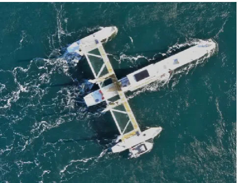
[image:2.595.307.551.51.170.2]The Sustainable Marine Energy Ltd. (SME) floating tidal energy device, PLAT-I (PLATform-Inshore), was used as a case study device in terms of power extraction and operational constraints. PLAT-I is attached to the seabed with SME rock anchors and catenary mooring lines leading to a flow aligning turret on the bow (Figure 1). It houses 4 in-stream turbines, each with a rated power of 70kW.
Figure 1. Operational PLAT-I tidal energy device.
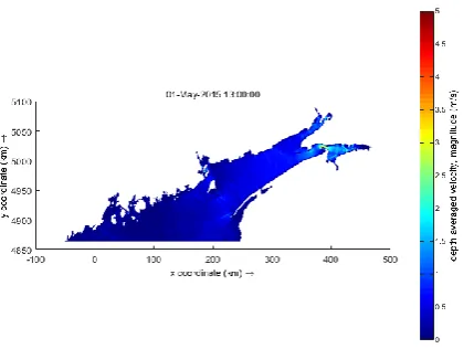
[image:2.595.46.289.458.644.2]The wider Bay of Fundy in Eastern Canada (Figure 2) was selected as a case study location, due to known hotspots of tidal energy and data availability for model validation.
Figure 2. Wider Bay of Fundy area, Eastern Canada.
The numerical modelling techniques utilised for this paper are not designed to be a perfect recreation of complex natural phenomena. Their purpose is to allow a tidal developer to make an informed initial choice between potential deployment locations; providing quantifiable inputs to a decision that was previously either not considered or burdened with a lack of data and high uncertainties. This is particularly important when targeting remote or lesser known sites.
B. Model Setup 1) Domain
The GEBCO bathymetry data is a continuous high-resolution terrain model generated from the interpolation of multiple databases of satellite data and ship-track soundings. The GEBCO dataset gives up to 20m resolution, which is sufficiently detailed for an initial site assessment, but is also limited in accuracy in areas that are not frequented by vessels, or areas of complex bathymetry. The data was loaded into the Delft3D-FM model using the WGS ‘84 (World Geodetic System) coordinate and a UTM (Universal Transverse Mercator) Zone 20T chart datum.
A single depth-layer computational grid of 1000x600x1 400m grid cells was generated over the bathymetry, with a time step of 15 seconds used to satisfy the Courant condition [11]. The water density was set to 1025kg/m3 to represent seawater, and a Chezy friction regime of 55 m1/2/s was
applied uniformly to represent a generally deep, rocky bed [12]. Horizontal eddy viscosity and diffusivity were uniformly set to 40m/s and 10m/s respectively, as values appropriate for the grid cell size [5]. All other physical and numerical parameters were left as default.
Historic Wind Velocity (W10) data for the duration of the
Figure 3. Wind Velocity input to Delft3D-FM domain.
Due to computational constraints, the simulation was initially run for the month of May 2015, but with the objective of modelling an annual cycle for the full paper submission.
2) Boundary Conditions
The Southern open boundary of the hydrodynamic simulation was forced astronomically using the TPXO 7.2 Global Inverse Tidal Model. This model provides gridded estimates of tidal coefficients by interpolating between constituents confirmed by active tide gauge stations. This boundary provides the driving force [14] to generate VD, the
depth-averaged flow velocities (Figure 4).
Figure 4. Delft3D-FM FLOW output of VD.
The Southern open boundary of the phase-averaging SWAN (Simulating WAves Nearshore) simulation was set to HS = 1m, Period (T) = 5.5s and Wave Direction (from) (Hd)
= 180°. This represents a moderately developed sea state in a deep area, that is not limited by fetch to the South [15]. Along with the wind inputs, this boundary generates the HS
outputs (Figure 5).
Figure 5. Delft3D-FM WAVE (SWAN) output of HS.
C. Calculating Operational Windows 1) Vessel Characteristics
[image:3.595.316.535.56.207.2]In order to calculate an approximation for weather window occurrences and durations, it is necessary to input transit, safe working conditions and other operational constraints into the calculations. Table 1 shows example constraints for a maintenance operation, based on SME operational experience with work boats and marine contractors.
Table 1. Maintenance Vessel Characteristics
2) Path to Port
For maintenance operations an appropriate port is also required. Within the domain designated in the smaller grid, several suitable ports have been identified. In order to estimate the transit distance and time for a marine operation, as well as the likely MetOcean conditions encountered, it is necessary to designate an efficient route from the nearest port to each point within the domain.
A Dijkstra's Algorithm was employed to find the shortest weighted path between two valid points on the grid. In this instance, valid criteria are designated as a) not land, and b) deep enough to transit through (5m depth). The weighting, or mobility, of the DA is the ease with which the algorithm will progress to the next point. At this juncture, depth alone was used as a mobility parameter to ensure the vessel kept to a shallow and typically sheltered route.
At each grid cell node along the algorithm path, the flow speed and significant wave height were output for every hour of the simulation. The probability of the transit limits being exceeded at any single node along the transit route, and the operational limits being exceeded at the deployment site node, can then be estimated.
The impacts of MetOcean conditions on transit time (travelling against flow/waves) is not included at this juncture but is planned for future iterations.
Limiting Parameter Transit Operation
Tidal Flow Speed (m/s) 3 1
Wind Speed (m/s) 15 15
[image:3.595.61.276.396.554.2]3) Neap Tide Identification
In areas with potential for tidal energy development, an ever-present constriction upon marine operations is the flow of the tide. Utilizing Table 1, vessels will be unable to operate in flow speeds of more than 1m/s, and it will be unsafe to transit through flow speeds of 3m/s. During fortnightly Spring (stronger) tides, the daily period of accessibility is relatively short, as the flow speed must remain below the vessel threshold for the duration of the marine operation. Lengthy O&M is often targeted to slack periods and planned to occur during neap (weaker) tides [16].
While this does not leave many available hours within a month for O&M, the tides are a highly predictable resource [17]. This means that the length and timing of the neap slack periods can be predicted months, or even years in advance through harmonic analysis (if historic data is available), or through the numerical modeling techniques discussed within this paper.
For use with Weibull Persistence Statistics (detailed in the following section), this effectively means that the model Duration (D) is reduced from 744 hours (in a month) to the number of hours during the fortnightly neap periods where the flow speed remains below the operational threshold for the length of the required O&M.
4) Weibull Persistence Statistics
Extracting time-varying MetOcean parameters at each node along the transit route, allows for the probability of operational thresholds being exceeded at any point during the journey to be calculated through a Weibull Persistence Method [9], [10]. By applying a Weibull Fit to the probability of exceedance of the MetOcean data, it is possible to identify the shape (k), scale (b) and location (X0)
parameters. The k parameter alters the shape of the distribution, such that it could take on the appearance of a bell curve, or exponentially tend towards zero or one. The scale parameter b focuses the density of the probability distribution into a smaller area. Finally, the location parameter shifts the distribution along the x-axis. It is defaulted to 0 and is only altered to provide a better fit to the raw probability of exceedance data. Having identified the Weibull Parameters k and b, the Weibull Probability of Exceedance (PW) can then be calculated (Equation 1).
(1) Where M is a MetOcean parameter such as HS, and MAcc
is the threshold operational limit for said parameter (Table 1). PW allows for the calculation of the average length of an
accessible weather window with designated operational
constraints (τAcc) (Equation 2).
(2) Where D is the model duration and Nω is the number of
weather windows within the modelled duration. For example, if a threshold operational limit was only exceeded twice separately during a month, then Nω= 3. The probability
that a normalised accessible weather window (Xi) will persist
as the Probability of Persistence (Equation 3). Xi is defined
as the operational length requirement divided by τAcc.
(3)
Where CAcc is the occurrence of accessible conditions as
derived from the Weibull distribution shape (Equation 4) and
αAcc is the relationship between the mean MetOcean value M ̅
and the threshold operation value MAcc (Equation 5),
assuming a linear correlation characteristic [18].
(4)
(5)
The γ coefficient (Equation 6) and M ̅ (Equation 7) are both derived from the Weibull distribution shape, scale and location parameters.
(6)
(7)
Combining the probabilities of Weibull Exceedance and Persistence allows for calculation of the occurrence of a weather window with both specified MetOcean limits and required duration (Equation 8).
(8)
D. Levelised Cost of Energy 1) Access & Waiting Hours
The Weibull distribution can be utilised to not only estimate the likelihood of a weather window occurring, but also the number of access hours (NAcc) in a given duration
that such windows will occur for (Equation 9), and how long it is likely that an operation will have to wait (NWait) before a
weather window occurs (Equation 10).
(9)
(10)
2) Power Generation & Electrical Losses
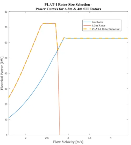
Power Generated (PG) will be calculated by utilising
numerically modelled flow velocities at the hub height of the PLAT-I turbines and the power curves [21] of the PLAT-I 6.3 and 4m turbines (Figure 6). An estimate of flow velocity at this depth was calculated from VD by splitting the depth at
[image:5.595.64.278.176.412.2]each point in the domain into 1m bins and assuming a 1/7th Law profile [22].
Figure 6. PLAT-I power curves for two rotor options.
Electrical Power Losses (PL) will be calculated as a
function of distance, PG and transmission parameters [23]
given below in Table 2. Grid connection points will be designated as moderately sized coastal towns within the domain.
Table 2. Electrical Transmission Parameters
Transmission Parameter Value
Generation Voltage (V) 400 Export Cable Voltage (V) 3300
Grid Voltage (V) 13800 PLAT-I Rated Power (kW) 280 Export Cable Cross Section (mm2) 10
Export Cable Resistance (ohm/km) 0.99 Water Temperature (°C) 8
De-rating (%) 107
Power Factor (%) 95
Transformer Efficiency (%) 96 Switchgear Efficiency (%) 99
3) Downtime
The completed paper will explore the monthly and annual loss of power extraction due to downtime, upon completion of the longer Delft3D-FM model runs. Total downtime during the deployment will be approximated as a total of three calculation processes:
1. Downtime due to planned marine operations. This is expected to be negligible, as if the maintenance is not essential, then rearranging the operation for a few days or even a month is unlikely to incur much loss of power generation. 2. Downtime due to non-completion of unplanned
marine operations. This will be highly sensitive to the selected deployment location. If faults/damage occurs, or if an unexpected but urgent repair is required, then there will be a period of downtime until the corrective O&M can be completed. MetOcean conditions will affect the viability of marine operations.
3. Downtime due to extreme MetOcean conditions. Again, this will be highly sensitive to the deployment location, and thus will vary spatially. If for safety or to prevent damage to components, power generation must be ceased repeatedly, then this will have an impact upon the downtime and total amount of power that can be exported. 4) Cost Assignment
A successful marine operation will incur all the cost estimates (A-E) given in Table 3. However, due to MetOcean constraints, planned marine operations rarely occur without delay or re-arrangement.
Table 3. Maintenance Operation Costs
Aspect of Operation Cost ($ USD)
A: Vessel Hire (per day) 4500 B: 2x Specialist Staff (per day) 1000 C: Vessel Standby (per day) 2500 D: Vessel Running (per hour) 500
E: Vessel Transit (per km) 100
The overall cost of re-scheduled operations can be calculated through four distinct methods, each of which is employed by marine contractors and professionals depending upon circumstance:
1. Decreasing Weather Window Contract – Early Decision. In this instance, if for example long-term weather forecasts initiate a decision to cancel an operation a week/fortnight before, then the operation can be rescheduled without added vessel costs. The only additional costs incurred are potentially the specialist staff costs (B) but has the risk of unnecessarily cancelling a vital operation.
[image:5.595.60.281.541.682.2]except that there is the option to incur a vessel standby (C) and staff costs (B) each day until the operation is successful. For infrequent but essential marine operations, this option is the most prevalent, despite the risk of a potentially prolonged and costly standby period. In this paper, the standby period will be calculated through the Weibull Persistence Method for waiting hours/days.
4. Permanent Standby Contract. This very different instance is most suited to a situation where many operations are required during the deployment period. A fixed monthly, quarterly, or even year-long contracted price is applied. Because vessel hire and standby costs are incorporated into the price, only the staff (B), vessel running (D) and transit (E) costs are incurred during each required operation.
Each of these methods will be costed for every potential deployment position within the Bay of Fundy. By applying several options for the number of O&M action required, it will be possible to identify an optimum operational regime, which will itself contribute to the selection of an optimum for a floating tidal energy converter in terms of LCoE.
ACKNOWLEDGMENTS
The authors wish to acknowledge the companies and funding bodies who have enabled the collection and interrogation of the data used in this paper, as well as allowing for its publication. Sustainable Marine Energy Ltd. have provided invaluable case study data and expertise. The software developers at Delft Deltares, GEBCO and DHI have developed vital modelling tools and data. The Industrial Doctoral Centre for Offshore Renewable Energy (IDCORE) and its contributing funding bodies have provided the authors with the facilities and financial backing to produce this paper.
REFERENCES
[1] R. Vennell, “Estimating the power potential of tidal currents and the impact of power extraction on flow speeds,”Renew. Energy, vol. 36, no. 12, pp. 3558–3565, 2011.
[2] R. Ahmadian and R. A. Falconer, “Assessment of array shape of tidal stream turbines on hydro-environmental impacts and power output,”Renew. Energy, vol. 44, pp. 318–327, 2012.
[3] J. Mcdowell, P. Jeffcoate, T. Bruce, and L. Johanning, “Numerically Modelling the Spatial Distribution of Weather Windows : Improving the Site Selection Methodology for Floating Tidal Platforms,” 2018.
[4] P. Jeffcoate, J. Mcdowell, and N. Cresswell, “Floating Tidal Energy Site Assessment Techniques for Coastal and Island Communities,” 2018.
[5] Deltares systems, “Delft3D-FLOW, User Manual,” pp. 1–684, 2014.
Cycle, p. 126, 2009.
[7] G. Egbert and L. Erofeeva, “TPXO global and local models,” pp. 2–3.
[8] J. D. H. Wiseman and C. D. Ovey, “The general bathymetric chart of the oceans,”Deep Sea Res., vol. 2, no. 4, pp. 269–273, 2008.
[9] C. Frost, D. Findlay, E. Macpherson, P. Sayer, and L. Johanning, “A model to map levelised cost of energy for wave energy projects,”Ocean Eng., vol. 149, no. January 2017, pp. 438–451, 2017.
[10] R. T. Walker, J. Van Nieuwkoop-Mccall, L. Johanning, and R. J. Parkinson, “Calculating weather windows: Application to transit, installation and the implications on deployment success,”Ocean Eng., vol. 68, pp. 88–101, 2013.
[11] F. Achete, “Morphodynamics of the Ameland Bornrif,” 2011. [12] T. A. D. Davey, V. Venugopal, F. Girard, H. C. M. Smith, G. H.
Smith, J. Lawrence, L. Cavaleri, L. Bertotti, M. Prevosto, and B. Holmes, “D2.7 Protocols for wave and tidal resource assessment,”EquiMar Protoc., 2010.
[13] F. Schlütter, O. S. Petersen, and L. Nyborg, “Resource Mapping of Wave Energy Production in Europe,” pp. 1–9, 2015.
[14] G. D. Egbert and S. Y. Erofeeva, “Efficient inverse modeling of barotropic ocean tides,”J. Atmos. Ocean. Technol., vol. 19, no. 2, pp. 183–204, 2002.
[15] A. Cooper and R. Mulligan, “Application of a Spectral Wave Model to Assess Breakwater Configurations at a Small Craft Harbour on Lake Ontario,”J. Mar. Sci. Eng., vol. 4, no. 3, p. 46, 2016.
[16] M. Morandeau, R. T. Walker, R. Argall, and R. F. Nicholls-Lee, “Optimisation of marine energy installation operations,”Int. J. Mar. Energy, vol. 3–4, pp. 14–26, 2013.
[17] Daniel Codiga, “"UTide" Unified Tidal Analysis and Prediction Functions - File Exchange - MATLAB Central,” 2017. [18] T. Stallard, J. F. Dhedin, S. Saviot, and C. Noguera, “D7.4.1 Procedures for estimating sit accessibility & D7.4.2 Appraisal of implications of site accessibility,”EquiMar Protoc., 2010. [19] T. Stallard and P. K. Stansby, “D7.3.1 Support Structures for
Arrays of Wave Energy Devices,”EquiMar Protoc., 2009. [20] J. Mcdowell, T. Bruce, and P. L. Johanning, “Numerical
Modelling of the Spatial Distribution of Revenue and O & M Costs for Floating Tidal Platforms,” 2017.
[21] P. Jeffcoate, R. Starzmann, B. Elsaesser, S. Scholl, and S. Bischoff, “Field measurements of a full scale tidal turbine,”Int. J. Mar. Energy, vol. 12, pp. 3–20, 2015.
[22] C. Legrand, Black and Veatch, and Emec, Assessment of Tidal Energy Resource. 2009.