City, University of London Institutional Repository
Citation
: Broom, M. & Rychtar, J. (2016). Nonlinear and Multiplayer Evolutionary Games.
Annals of the International Society of Dynamic Games, 14, pp. 95-115. doi:
10.1007/978-3-319-28014-1_5
This is the accepted version of the paper.
This version of the publication may differ from the final published
version.
Permanent repository link:
http://openaccess.city.ac.uk/15851/
Link to published version
: http://dx.doi.org/10.1007/978-3-319-28014-1_5
Copyright and reuse:
City Research Online aims to make research
outputs of City, University of London available to a wider audience.
Copyright and Moral Rights remain with the author(s) and/or copyright
holders. URLs from City Research Online may be freely distributed and
linked to.
City Research Online: http://openaccess.city.ac.uk/ [email protected]
Nonlinear and multiplayer evolutionary games
Mark Broom and Jan Rycht´aˇr
AbstractClassical evolutionary game theory has typically considered populations within which randomly selected pairs of individuals play games against each other, and the resulting payoff functions are linear. These simple functions have led to a number of pleasing results for the dynamic theory, the static theory of evolutionar-ily stable strategies, and the relationship between them. We discuss such games, to-gether with a basic introduction to evolutionary game theory, in Section 1. Realistic populations, however, will generally not have these nice properties, and the payoffs will be nonlinear. In Section 2 we discuss various ways in which nonlinearity can appear in evolutionary games, including pairwise games with strategy-dependent interaction rates, and playing the field games, where payoffs depend upon the en-tire population composition, and not on individual games. In Section 3 we consider multiplayer games, where payoffs are the result of interactions between groups of size greater than two, which again leads to nonlinearity, and a breakdown of some of the classical results of Section 1. Finally in Section 4 we summarise and discuss the previous sections.
Key words: ESS; payoffs; matrix games; nonlinearity; multi-player games
MSC codes:91A22; 91A06; 91A80; 92B05
Mark Broom
Department of Mathematics, City University London, Northampton Square, London, EC1V 0HB, UK, e-mail:[email protected]
Jan Rycht´aˇr
Department of Mathematics and Statistics, The University of North Carolina at Greensboro, Greensboro, NC 27412, USA, e-mail:[email protected]
1 Introduction
In this paper we consider nonlinear and multiplayer evolutionary games. We start in Section 1 with an introduction to evolutionary games for those not familiar with them, focusing on matrix games, which are linear in character, and discussing a number of the key results. We then move on to consider the general idea of non-linear evolutionary games, including some specific types of such games in Section 2. We believe that these results, and those in the following section, will generally be less familiar to the audience. In Section 3 we consider multiplayer games. The specific type that we consider, and the most commonly used, is multiplayer matrix games, which can be though of as a special type of the nonlinear games in Section 2, although we note that multiplayer games in general do not simply reduce to this type. The text in significant part follows a tutorial talk given by MB at the Interna-tional Society on Dynamic Games Symposium in Amsterdam in July 2014, which in turn followed aspects of the book Broom and Rycht´aˇr (2013).
1.1
What is evolutionary game theory?
Evolutionary game theory as we know it today began in the 1960s, in particular with the consideration of the sex-ratio problem (Hamilton, 1967), although similar reasoning on this problem goes back much earlier to Dusing (see Edwards, 2000) and Fisher (Fisher, 1930). The most influential work on our modern understand-ing is that of Maynard Smith and collaborators (Maynard Smith and Price, 1973; Maynard Smith, 1982).
In (non-cooperative) game theory, a game is comprised of three key elements, the players, thestrategiesavailable to be employed by the players, and thepayoffsto the players, which are functions of the strategies chosen. For an evolutionary game we also need apopulation, and a way for our population to evolve through time, an evolutionary dynamics.
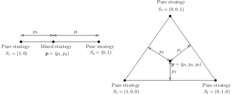
Apure strategyis a choice of what to play in a given interaction. Supposing that the pure strategies comprise the finite set{S1,S2, . . . ,Sn}, then a mixed strategy is
defined as a probability vectorp= (p1,p2, . . . ,pn),pibeing the probability that the
player will play pure strategySi. Thus a pure strategy can be written in this way, e.g.
Siis(0, . . . ,0,1,0, . . . ,0)with 1 at theithplace, and a mixed strategy can be written
as a convex combination of pure strategies,
p= (p1,p2, . . . ,pn) = n
∑
i=1
piSi. (1)
The set of all mixed strategies can be represented by a simplex inRnwith vertices at{S1,S2, . . . ,Sn}. TheSupport ofp,S(p), is defined byS(p) ={i:pi>0}, so that
it is the set of pure strategies which have a positive probability of being played by a
the set of pure strategies is infinite, as in the “war of attrition” game, for example Bishop and Cannings (1978).
Pure strategy Mixed strategy Pure strategy S1= (1,0) p= (p1, p2) S2= (0,1)
p2 p1
Pure strategy Pure strategy Pure strategy
S1= (1,0,0) S2= (0,1,0)
S3= (0,0,1)
p1
p3
p2
p= (p1, p2, p3)
Fig. 1 Visualization of pure and mixed strategies for games with two or three strategies.
Payoffs for a game played by two players with each having a finite number of pure strategies can be represented by two matrices. For example, if player 1 has the strategy setS={S1, . . . ,Sn}and player 2 has the strategy setT={T1, . . . ,Tm}, then
the payoffs in this game are written as
A= (ai j)i=1,...,n;j=1,...,m,B= (bi j)i=1,...,m;j=1,...,n, (2)
whereai j(bji) is the reward to players 1 (2) after player 1 (2) chooses pure strategy
Si(Tj). We thus have the payoffs written as a pair ofn×mmatricesAandBT, which
is known as a bimatrix representation. This is often written as a single matrix whose entries are ordered pairs of values.
Note that here we write the payoffs from the point of view of the player receiving the reward (i.e. the index of their strategy comes first). It is often the case in other works that the index of player 1 is written first.
Often in evolutionary games, the choice of which player is player 1 is arbitrary, and thus the strategies available to the two players are identical. In this case,n=m and (after a possible renumbering)Si=Tifor alli. Since the ordering of players is
arbitrary, if we swap them their payoffs are unchanged, so thatbi j=ai j, i.e.A=B.
This means that all payoffs can be written as a singlen×nmatrix
A= (ai j)i,j=1,...,n, (3)
where in this case,ai j is the payoff to a player playing pure strategySi when its
opponent plays strategySj. Such a game is called amatrix game.
Consider a game with payoffs given by a matrixA. If player 1 playspand player 2 playsq, then the proportion of games involving the first player playingSiand the
second player playingSj is simply piqj. The expected reward to player 1 is thus
given by
E[p,q] =
∑
i,j
[image:4.612.183.422.140.237.2]Note that, when comparing payoffs, we can ignore difficult cases involving
equal-ities by assuming our games aregeneric(Samuelson, 1997; Broom and Rycht´aˇr,
2013). In most of the following we will make this assumption.
In the above, we have considered a single game between two individuals. How-ever, evolutionary games consist of populations, and individuals are not (usually) involved in only a single contest. They may play many different contest, against many different opponents, with each contributing a relatively small contribution to the total reward.
We consider a functionE[σ;Π], the fitness of an individual using a strategyσin
a population represented byΠ. The termδpis used to represent a population where
the probability of a randomly selected player being a p-player is 1. The term δi
similarly denotes a population consisting only of individuals playing pure strategySi
(with probability 1). The term∑ipiδithus means a population where the proportion
ofSi-playing individuals ispi.
1.2
Two approaches to game analysis
1.2.1 Dynamic analysis
In all that follows we assume a very large (effectively infinite) population, with overlapping generations and asexual reproduction, where offspring are direct copies of their parent. The evolution of a population can be modelled using evolutionary dynamics, where the proportion of individuals playing a given strategy changes ac-cording to their fitness.
In the following we shall assume a population consisting only of pure strategists. Thus we consider a population represented bypT=∑ipiδi, i.e. where the frequency
ofSi-playing individuals ispi. We denote the fitness of individuals playingSiin this
population to be fi(p). The birth rate of individuals in the population is proportional
to their fitness.
We assume that the composition of the population changes according to the dif-ferential equation
d dtpi=pi
fi p(t)
−f¯(p(t)). (5) This is thecontinuous replicator dynamics, the most commonly used evolutionary dynamics, originating in Taylor and Jonker (1978) (see also Hofbauer and Sigmund, 1998). For a derivation see Broom and Rycht´aˇr (2013). We also note the existence of the discrete replicator dynamics, the equivalent dynamics for non-overlapping generations (see Bishop and Cannings, 1978).
For matrix games the continuous replicator dynamics (5) becomes
d dtpi=pi
A p(t)T
i−p(t)A p(t)
T
1.2.2 Static analysis
An alternative methodology is to use a static analysis, which does not consider how the population reached a particular point in the strategy space, but assuming that the population is at that point, asks whether other strategies can do better within the population?
Consider a population where the vast majority of individuals play strategy S, while a very small proportion ε>0 of “mutants” play strategy M. The
strate-gies S andM thus compete within the population (1−ε)δS+ε δM. A strategyS
isevolutionarily stable against strategyMif there isεM>0 such that
E[S;(1−ε)δS+ε δM]>E[M;(1−ε)δS+ε δM] (7)
for all ε<εM.S is an evolutionarily stable strategy (ESS)if it isevolutionarily
stable againstM for every other strategyM6=S (Maynard Smith and Price, 1973; Maynard Smith, 1982).
For matrix games, the linearity of the payoffs gives
E[p;(1−ε)δp+ε δq] =E[p,(1−ε)p+εq] = (8)
pA((1−ε)p+εq)T= (1−ε)pApT+εpAqT. (9)
It is easy to show that this means a strategypis anEvolutionarily Stable Strategy (ESS)for a matrix game, if and only if for any mixed strategyq6=p
E[p,p]≥E[q,p], (10)
IfE[p,p] =E[q,p], thenE[p,q]>E[q,q], (11) (see e.g. Broom and Rycht´aˇr, 2013).
We note that inequality (10) is the Nash equilibrium condition, but that, while necessary, it is not sufficient for stability. If (11) does not hold, thenpmay be in-vaded by a mutant that does equally well against the majority of individuals in the population (that playp) but gets a (tiny) advantage against them by outperforming them in the (rare) contests with other mutants (playingq).
Alternatively there is the possibility that the mutant and the residents do equally well against the mutants too. In this latter case invasion can occur by “drift”; both types do equally well, so in the absence of selective advantage random chance de-cides whether the frequency of mutants increases or decreases.
We defineT(p)as the set of pure strategies with equal payoffs againstp, i.e. T(p) ={i:E[Si,p] =E[p,p]}. (12) Theorem 1 (Bishop Cannings Theorem).Ifpis an ESS of the matrix game A and
1.2.3 Dynamic versus static analysis
Dynamic and static analyses are mainly complementary, however the relationship between the two is not straightforward, and there is some apparent inconsistency between the theories. Comparing the static ESS analysis and replicator dynamics, we see that the information required for each type of analysis is different. To
deter-mine whetherpis an ESS, we need the minimum of a function
q→E[p;(1−ε)δp+ε δq]−E[q;(1−ε)δp+ε δq] (13)
to be attained forq=pfor all sufficiently smallε>0.
To understand the replicator dynamics, however, we needE[Si;pT]for alliand
allp. Thus a major difference between the two methods is that the static analysis considers monomorphic populationsδpwhile the dynamic analysis considers mixed
populationspT=∑ipiδi.
The analyses can thus produce the same (or at least similar) results only if there is an identification betweenδpandpT, as in the case of matrix games, and we note that
most of the comparative analysis between the methods has assumed matrix games.
Theorem 2 (Folk theorem of evolutionary game theory, Hofbauer and Sigmund (2003)).For a matrix game with payoffs given by matrix A, we have:
1) Ifpis a Nash equilibrium, and so an ESS, of a matrix game, thenpT is a rest point of the dynamics , i.e. the population does not evolve further from the state
pT=
∑ipiδi.
2) Ifpis a strict Nash equilibrium, thenpis locally asymptotically stable.
3) If the rest pointp∗of the dynamics is also the limit of an interior orbit, then it is a Nash equilibrium.
4) If the rest pointpis Lyapunov stable, thenpis a Nash equilibrium.
An ESS is an attractor of the replicator dynamics, and the population converges to the ESS for every strategy sufficiently close to it. Ifp is an internal ESS, then global convergence topis assured (Zeeman, 1980).
It is also true that if the replicator dynamics has a unique internal rest pointp∗, under certain conditions (satisfied for matrix games)
lim
t→∞ 1 T
Z T
0
pi(t)dt=p∗i, (14)
so that the long-term average strategy is given by this rest point, even if there is considerable variation at any given time.
Thus for matrix games, identifying ESSs and Nash equilibria of a game gives a lot of important information about the dynamics. For example, ifp is an internal ESS, then global convergence topis assured.
0 1 −1
−2 0 2
2 −1 0
. (15)
(see Hofbauer and Sigmund, 1998). The replicator dynamics for this game has a unique internal attractor, but this attractor is not an ESS. This happens because we can find an invading mixture forpwhere the dynamics effectively forces the mixture into a combination that no longer invades. Thus if the invading group is comprised of mixed strategists it can invade, whereas if it is comprised of a mixture of pure strategists it cannot. Note that for the discrete dynamics the situation is even more complex, since then it is not guaranteed that an ESS is an attractor (Cannings, 1990).
1.3
Two classic matrix games
Two well-known examples of matrix games are the Hawk-Dove game (Maynard Smith and Price, 1973) and the prisoner’s dilemma (Tucker, 1980). These both represent important biological/ social scenarios.
1.3.1 The Hawk Dove game
For the Hawk-Dove game, individual compete against other randomly chosen indi-viduals for a reward (e.g. a territory) of valueV >0. Each of the contestants has two pure strategies available, Hawk (H) and Dove (D). Hawks fight, whereas Doves merely display. Doves divide the reward, a Hawk always beats a Dove, whereas two Hawks fight, with the loser incurring a cost C. This gives the payoff matrix as
Hawk Dove
Hawk V−C
2 V
Dove 0 V
2
. (16)
Denoting a mixed strategyp= (p,1−p)to mean to play Hawk with probability p and to play Dove otherwise, it is easy to show that pure Dove is never an ESS, pure Hawk is an ESS ifV ≥C. ForV<C,p= (V/C,1−V/C)is the unique ESS (see e.g. Broom and Rycht´aˇr, 2013).
1.3.2 The prisoner’s dilemma
Cooperate De f ect
Cooperate R S
De f ect T P
. (17)
Whilst the individual numbers are not important, for the classical dilemma we need T>R>P>S. We also need the additional condition 2R>S+Twhich is necessary for the evolution of cooperation. In this game Defect is the unique ESS, although if both players cooperated they would do better. The game is widely used to consider the issue of (especially human cooperation), and of how it can be established against cheating. Many variants of the above game, usually using multiple interactions of some kind, have been developed to this end (see e.g. Axelrod, 1981; Nowak, 2006).
2 Nonlinear games
2.1
Overview and general theory
In the previous section we considered matrix games, where
E[p;qT] =pAqT. (18)
The above payoffs can alternatively be written in the form∑ipi(AqT)ior∑j(pA)jqj,
and so payoffs are linear in both the strategy of the focal individual and the strategy of the population and, as we have seen, this has nice static and dynamic properties. More generally, we say thatE islinear on the leftif it is linear in the strategy of the focal player, i.e.
E
"
∑
i αipi;Π
#
=
∑
i
αiE[pi;Π] (19)
for every populationΠ, everym−tuple of individual strategiesp1, . . . ,pmand every
collection of constantsαi≥0 such that∑iαi=1 (Broom and Rycht´aˇr, 2013).
We say thatE islinear on the rightif it is linear in the strategy of the population, i.e.
E
"
p;
∑
i αiδqi
#
=
∑
i
αiE[p;δqi] (20) for every individual strategyp, everym−tupleq1, . . . ,qm and every collection of αi’s from[0,1]such that∑iαi=1 (Broom and Rycht´aˇr, 2013).
Recall that for matrix games, the payoff to an individual is the same whether it faces opponents playing a polymorphic mixture of pure strategies or a monomorphic
population. We say that a game haspolymorphic-monomorphic equivalenceif for
E
"
p;
∑
i αiδqi
#
=Ep;δ∑iαiqi
, (21)
(Broom and Rycht´aˇr, 2013). Note that he concept of polymorphic-monomorphic equivalence holds only in respect of static analyses, and there is no such concept in terms of dynamics.
The payoff is linear on the left for many evolutionary games becauseE[p;Π]is
often defined to be the average of the payoffs to players of pure strategySi, weighted
by the selection probability pi, for alli. It is common, however, that the payoff is
nonlinear on the right, which occurs whenever the game does not involve pairwise contests against randomly selected opponents.
The payoff function can be nonlinear on the left, if a strategy is a pure strategy drawn from a continuum, but that the payoff is nonlinear as a function of this pure strategy, such as in the tree height game from Kokko (2007) that we consider in Section 2.4. Nearly all real situations feature nonlinearity of some type, and when models of real behaviours are developed, the payoffs involved are indeed generally nonlinear in some way.
Some results for linear games can be generalized and reformulated for nonlinear games. The conditions (10) and (11) can be generalized as follows:
Theorem 3.For games with generic payoffs, if the incentive function
hp,q,u=E[p;(1−u)δp+uδq]−E[q;(1−u)δp+uδq] (22)
is differentiable (from the right) at u=0for everypandq, thenpis an ESS if and only if for everyq6=p;
1.E[p;δp]≥E[q;δp]and
2. ifE[p;δp] =E[q;δp], then ∂∂u
(u=0)hp,q,u>0. For a proof, see (Broom and Rycht´aˇr, 2013).
Theorem 4.Let E be linear in the focal player strategy, i.e. (19) holds, and let the function hp,q,ube differentiable w.r.t u at u=0. Letp= (pi)be an ESS. Then
E[p;δp] =E[Si;δp]for any pure strategy Sisuch that i∈S(p) ={j;pj>0}.
For a proof see Broom and Rycht´aˇr (2013). We note that it is enough to assume hp,q,uto be continuous.
If the payoff is not linear but strictly convex so that, for allqand allpwith at least two elements inS(p),
∑
i
piE[Si;δq]>E[p;δq], (23)
Lemma 1 below shows that the payoffs of games that are linear in the focal player strategy and satisfy polymorphic monomorphic equivalence (21) must be of a special form. These games are calledpopulation games, orplaying the field games.
Lemma 1.If the payoffs of the game are linear in the focal player strategy (i.e. satisfy (19)) and satisfy polymorphic monomorphic equivalence (21), then for every
x,y,zand everyε∈[0,1]
E[x;(1−ε)δy+ε δz] =
∑
i
xifi (1−ε)y+εz (24)
where fi(q) =E[Si;δq].
Below we write payoffs in the formE[p;δq] =∑ipifi(q)for some functions fi,
and this indicates that payoffs are linear in the focal player strategy and also satisfy polymorphic monomorphic equivalence.
Theorem 5.Let the payoffs be such thatE[p;δq] =∑ipifi(q)for some continuous
functions fi. Then the strategypis an ESS if and only if it is locally superior, i.e.
there is U(p)a neighbourhood ofpsuch that
E[p;δq]>E[q;δq], for allq(6=p)∈U(p). (25)
For a proof, see Palm (1984).
2.2
Playing the field
In this section we consider payoff functions of the form
E[p;Π] =
∑
pifi(Π) (26)where the fi’s are (in general nonlinear) functions of the population strategy Π.
Such playing the field games are the most natural way of incorporating nonlinearity into a game model, since the fitness function automatically includes the population frequencies of the different strategies.
An example is the sex ratio game, one of the classical models of evolutionary game theory (Hamilton, 1967). The model considers the question of why the sex ratio in most animals is close to a half? At first sight there needs to be far less males than females, since often the only male contribution is in mating; in many species most offspring are fathered by a small number of males and the rest make no contribution.
one mother and one father, if generation sizes remain constant it is easy to show that the fitness of an individual with strategypis given by
E[p;δm] =
p m+
1−p
1−m (27)
so that in the notation of equation (26) we have
f1(m) = 1
m,f2(m) = 1
1−m. (28)
The unique ESS of this game ism=1/2, i.e. an equal sex ratio. The sex ratio game is in fact effectively just a special case of the following foraging problem (with N=2 andr1=r2).
Consider a population of animals foraging on N food patches, with resources
ri>0 per unit time fori=1, . . . ,N, equally shared by all individuals on the patch
(Parker, 1978).
The game hasNpure strategies for this game, each corresponding to foraging on a given patch, and a mixed strategyx= (xi)means to forage at patchiwith
prob-abilityxi. The payoff to an individual using strategyx= (xi)against a population
playingy= (yi)is
E[x;δy] =
∞, ifxi>0 for someisuch thatyi=0, N
∑
i;xi>0 xi
ri
yi
otherwise. (29)
It is clear from (29) that any ESSpmust havepi>0 for alli=1, . . . ,N. Thus any
potential problems with infinite payoffs do not need to be considered. In particular Theorem 3 holds despite the discontinuities in the fitness functions, since they are continuous in the vicinity of any potential ESS.
The unique ESSp= (pi)is given bypi=ri/∑Ni=1ri. This solution can
alterna-tively be written as
pi
pj
= ri
rj
. (30)
This is calledParker’s matching principle.
We can show this as follows. It is clear thatE[q;δp] =E[p;δp]for allq.
More-over, since this game satisfies polymorphic monomorphic equivalence (21) then
E[x;(1−u)δy+uδz] =E[x;δ(1−u)y+uz] (31)
and so
hp,q,u=E[p;(1−u)δp+uδq]−E[q;(1−u)δp+uδq] = (32)
N
∑
i=1
(pi−qi)
ri
pi+u(qi−pi)
N
∑
i=1 pi−qi
pi
ri
1−uqi−pi pi
+. . .
. (34)
This implies that
∂
∂u
u=0hp,q,u=
N
∑
i=1 ri
pi−qi
pi
2
>0. (35)
So from Theorem 3,pis an ESS.
2.3
Nonlinearity due to non-constant interaction rates
Another way for nonlinear games to occur is where the strategies employed by the players affect the frequency of their interactions. The pairwise interactions may be simple, but if the strategy affects the interaction rate, then the overall payoff function can be complicated.
The simplest non-trivial scenario is a two player contest with two pure strategies S1andS2, with payoffs given by the usual payoff matrix
a b c d
, (36)
but where the three types of interaction happen with probabilities not proportional to their frequencies.
Assume that each pair ofS1individuals meet at rater11, each pair ofS1andS2 individuals meet at rate r12 and each pair of S2 individuals meet at rater22 (see Taylor and Nowak, 2006). This yields the following nonlinear payoff function
E[S1;pT] =arr11p1+br12p2
11p1+r12p2 , (37)
E[S2;pT] = crr12p1+dr22p2
12p1+r22p2 . (38)
This reduces to the standard payoffs for a matrix game for the caser11=r12=r22. In the standard game with uniform interaction rates, ifa<candb>dthere is a mixed ESS, and this is also true for non-uniform interaction rates, although the ESS proportions change. Ifa>candb<dthen there are two ESSs in the uniform case, and this is also true for non-uniform interactions, although we note that the location of the unstable equilibrium between the pure strategies changes.
Otherwise for the uniform case there is a unique ESS. For non-uniform interac-tion rates, there is always a single pure ESS, but sometimes there is a mixed ESS too. Forc>a>d>b, and settingr12=1, this occurs if
r11r22>
p
(a−b)(c−d) +p(a−c)(b−d)
d−a
!2
The Prisoner’s Dilemma is an example wherec>a>d>b. Settingr11=r22=r and lettingr→∞the proportion of cooperators in the mixture tends to 1 and the basin of attraction of the proportion of cooperatorspin the replicator dynamics in-creases, tends top∈(0,1]. Thus in extreme cases, the eventual outcome of the game can be effectively the opposite to that implied by the game with uniform interaction rates.
2.4
Nonlinearity in the strategy of the focal player
Here we consider a third case, involving games where the strategy of an individual is described by a single number (or a vector) that does not represent the probability of playing a given pure strategy, but rather represents a unique behaviour such as the intensity of a signal. We note that this is also the scenario generally considered in Adaptive Dynamics (see e.g. Metz et al, 1992; Metz, 2008), though in practice stronger assumptions are generally made than we use here.
Consider the following game-theoretical model of tree growth Koch et al (2004); Kokko (2007). We assume that a tree has to grow large enough in order to get sun-light and not get overshadowed by neighbours; yet the more the tree grows the more of its energy has to be devoted to “standing” rather than photosynthesis.
Let h∈[0,1]be the normalized height of the tree, so that 1 is the maximum possible height of a tree. In Kokko (2007), the fitness of a tree of heighthin a forest where all other trees are of heightHwas given by
E[h;δH] = (1−h3)· 1+exp(H−h)
−1
, (40)
wheref(h) =1−h3represents the proportion of leaf tissue of a tree of heighthand g(h−H) = 1+exp(H−h)−1
represents the advantage or disadvantage of being taller/ shorter than neighbouring trees.
What are the ESSs for the tree, i.e. the evolutionarily stable heights? Differenti-ating (40) with respect tohobtains the unique maximum forh, i.e. the best response to a givenH in the population. Any ESS must be a best response to itself, and so settingh=Hafter the above differentiation yields
1
4 −6H
2+ (1−H3)
=0. (41)
3 Multi-player games
In the previous sections we have considered games with two individuals only, or games played against “the population”. We shall now consider situations with con-tests involving groups of individuals which are of size three or larger, selected ran-domly from a large population. We shall only consider multi-player matrix games (Broom et al, 1997) here. Note that another important example of a multi-player game is the multi-player war of attrition (Haigh and Cannings, 1989). For an exten-sive review of multiplayer evolutionary games, see Gokhale and Traulsen (2014).
3.1
Introduction to multi-player matrix games
Consider an infinite population, from which groups of m players are selected at random to play a game. The expected payoff to an individual is obtained by simply averaging over the rewards for all possible cases, weighted by their probabilities, as for matrix games.
In general where the ordering of individuals matter, extending the bimatrix game case tomplayers, the payoff to each individual in positionkis governed by an m-dimensional payoff matrix. However, as in matrix games, as opposed to bimatrix games, we assume that there is no significance to the ordering of the players. Thus an individual’s payoff depends only upon its strategy and the combination of its op-ponents’ strategies. We will call such gamessymmetric, and we have the following symmetry conditions:
ai1...im=ai1σ(i2)...σ(im) (42) for any permutationσ of the indicesi2, . . . ,im. For the three player case, these are
simply
apqr=aprq, for allp,q,r=1,2, . . . ,n. (43)
The payoff to an individual playing p in a contest with individuals playing
p1,p2, . . . ,pm−1respectively is written asE[p;p1,p2, . . . ,pm−1]. As the ordering is irrelevant, for convenience when some strategies are identical we use a power nota-tion, for exampleE[p;p1,p2,p3m−3].
The payoffs function is given as follows
E[p;p1,p2, . . . ,pm−1] =
n
∑
i=1 pi
n
∑
i1=1
· · ·
n
∑
im−1=1
aii1i2...i(m−1)
k−1
∏
j=1
pj,ij, (44)
wherepj= (pj,1,pj,2, . . . ,pj,n).
of the ordered positions. In particular the termai jkhas identical weighting toaik jin
the payoff to ani-player, so that the sum of these two can be replaced by twice their average.
A multi-player matrix is super-symmetric if
ai1...im =aσ(i1)...σ(im) (45) for any permutationσ of the indicesi1, . . . ,im.
For example, for super-symmetric three-player three strategy games, there are ten distinct payoffs. Without loss of generality we can define the three payoffsa111= a222=a333=0, and this leaves seven distinct payoffs to considera112,a113,a221,a223, a331,a332anda123. Broom et al (1997) considers the replicator dynamics for such games in detail, including every case where the last seven payoffs above take values of either 1 or -1. We will only discuss the simpler two strategy games here.
3.2
ESSs in multi-player matrix games
A strategypin anm-player game is calledevolutionarily stable against a strategy
qif there is anεq∈(0,1]such that for allε∈(0,εq]
E[p;(1−ε)δp+ε δq]>E[q;(1−ε)δp+ε δq], (46)
where
E[x;(1−ε)δy+ε δz] =
m−1
∑
l=0
m−1 l
(1−ε)lεm−1−lE[x;yl,zm−1−l]. (47)
p is anESS for the game if for everyq6=p, there is εq>0 such that (46) is
satisfied for allε∈(0,εq](Broom et al, 1997).
Similarly as in inequalities (10) and (11), we have the following:
Theorem 6.For an m-player matrix game, the mixed strategyp is evolutionarily stable againstqif and only if there is a j∈ {0,1, . . . ,m−1}such that
E[p;pm−1−j,qj]>E[q;pm−1−j,qj], (48) E[p;pm−1−i,qi] =E[q;pm−1−j,qi]for all i<j. (49) For a proof see Broom et al (1997) or Bukowski and Mie¸kisz (2004).
A strategypis anESS at level Jif, for everyq6=p, the conditions (48-49) of Theorem 6 are satisfied for some j≤Jand there is at least oneq6=pfor which the conditions are met for j=Jprecisely.
Ifpis an ESS, then by Theorem 6, for allq,
The payoffs are linear on the left so that
E[p;pm−1] =E[q;pm−1], for allqwithS(q)⊆S(p). (51) We note that in the generic case, any pure ESS is of level 0. A mixed ESS cannot be of level 0, but in the generic case, any mixed ESS must be of level 1.
Analogues of the strong restrictions on possible combinations of ESSs for ma-trix games do not hold for multi-player games. In particular, the Bishop-Cannings Theorem fails already form=3. Form>3, there can be more than one ESS with the same support as we shall see in Section 3.3. On the other hand, we still have the following form=3.
Theorem 7.It is not possible to have two ESSs with the same support in a three player matrix game.
For a proof, see Broom et al (1997) or Broom and Rycht´aˇr (2013).
3.3
Two-strategy multi-player games
We shall now consider games with only two pure strategies. The possible situations for a given individual are thus all combinations of that individual playing pure strat-egyi=1,2 againstm−1 players, jof which play strategyS1(and the otherm−1−j play strategyS2), for any 0≤j≤m−1. We shall denote these payoffs byαi j.
We consider an individual playing strategyxin a population playingy. A group ofm−1 opponents is chosen and each one of them chooses to play strategyS1with probabilityy1( and so strategyS2with probabilityy2=1−y1). We obtain
E[x;δy] =
m−1
∑
l=0
m−1
l
yl1ym2−1−lE[x;Sl1Sm2−1−l], (52)
where
E[x;Sl1,Sm2−1−l] =
2
∑
i=1
xiαil. (53)
Note that it does not matter whether the population is polymorphic or monomor-phic and playing the mean strategy; thus multi-player matrix games have the polymorphic-monomorphic equivalence property.
Recalling that the payoffs of them-player two strategy matrix game areαil for
i=1,2 andl=0,1, . . . ,m−1, we defineβl=α1l−α2l and consider the incentive
function
h(p) =E[S1;δ(p,1−p)]−E[S2;δ(p,1−p)] (54)
=∑ml=0−1
m−1
l
The functionh quantifies the benefits of using strategyS1over strategyS2in a population where all other players use strategyp= (p,1−p). Note thathis differ-entiable, and that the replicator dynamics now becomes
dq
dt =q(1−q)h(q). (56)
Theorem 8.In a generic two strategy m-player matrix game
1. pure strategy S1is an ESS (level 0) if and only ifβm−1>0, 2. pure strategy S2is an ESS (level 0) if and only ifβ0<0, 3. an internal strategyp= (p,1−p)is an ESS, if and only if 1. h(p) =0, and
2. h0(p)<0.
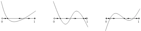
It is shown in Broom et al (1997) that the possible sets of ESSs are the following:
1. 0 pure ESSs, andlinternal ESSs withl≤ bm
2c; 2. 1 pure ESS, andlinternal ESSs withl≤ bm
2−1c;
3. 2 pure ESSs, andlinternal ESSs withl≤ bm
2−2c.
0 1 0 1 0 1
Fig. 2 The incentive function and ESSs in multiplayer games. The full dots show equilibrium
points and the arrows show the direction of the evolution under the replicator dynamics.
There can be more than one ESS with the same support in a 4-player game as shown in the example below.
Consider an example with the following payoffs (Bukowski and Mie¸kisz, 2004): withα11=α22=−1396,α13=α20=−323 andα10=α12=α21=α23=0. Thus
β0=3/32,β1=−13/96,β2=13/96,β3=−3/32 giving
h(p) =−3
32p
3+13
32p
2(1−p)−13
32p(1−p)
2+ 3
32(1−p)
3= (57)
−
p−1
4 p−
1
2 p−
3 4
. (58)
[image:18.612.183.418.372.424.2]4 Discussion
In this paper we have considered two main recent developments in the theory of evo-lutionary games. In particular the extension from linear matrix games to nonlinear games, and from two player to multiplayer games.
Nonlinearity within evolutionary games is introduced in its most natural way by considering games played against the population as a whole, so-called playing the field games. These can be generally expressed in the form of equation 26. They often result from situations where individuals do not interact directly, but where their behaviours have a direct effect on the environment, which then affects the payoffs of individuals. Thus in foraging models, the value of food patches depends directly on the intensity of their use by foragers within the population, as we saw from (Parker, 1978). More recent and realistic models of this phenomenon are given in Cressman et al (2004); Kˇrivan et al (2008) for example.
Even when games are pairwise, linearity only occurs because opponents are cho-sen at random, with equal probability. If some opponents are more likely than oth-ers and this is in any way related to the strategy of those involved, either through individuals directly being more likely to interact with those choosing a particular strategy or because evolution has led to different strategy distributions in differ-ent geographical locations, then nonlinearity will result, as we saw in Taylor and Nowak (2006). An example of this phenomenon occurs in food-stealing games, see e.g. Broom et al (2004, 2008).
The above games are linear in the strategy of the focal player, as its strategy is a probabilistic weighting of distinct choices. When its strategy is a single trait chosen from a continuum, such as the height of a tree as in Koch et al (2004); Kokko (2007), then there is nonlinearity in the focal player strategy too. Another example is the sperm allocation games of Parker et al (1997); Ball and Parker (2007). We also note that this idea is central to the related concept of adaptive dynamics, where populations evolve by successive small mutations, see Kisdi and Mesz´ena (1993); Geritz et al (1998).
Multiplayer games have been, and continue to be, common in Economics, for instance see Kim (1996),Wooders et al (2006), Ganzfried and Sandholm (2009). However until recently they have been less common in evolutionary games. An extension of the classical idea of well-mixed populations of pairwise games to con-sider such populations with multiplayer games was first introduced with the work of Palm (1984) and followed by Haigh and Cannings (1989); Broom et al (1997); Bukowski and Mie¸kisz (2004). More recently Hauert et al (2006), Gokhale and Traulsen (2010), Han et al (2012), Gokhale and Traulsen (2014) have developed the theory further.
As for nonlinear games above, multiplayer games can occur from non-independent pairwise games, for example within the formation of dominance hierarchies, where the results of a contest directly dictate who an individual will face next (if anybody). This was the focus of the games from Broom et al (2000a,b).
to deal with the stochastics effects which are not present in infinite populations, and where the single most important concept is that of the fixation probability of a rare mutant (equivalent to a small fraction of mutants within an infinite population, whose establishment within a population is either certain or impossible), impor-tant examples include Fogel et al (1998); Nowak et al (2004); Taylor et al (2004); Traulsen et al (2005); Nowak (2006). Within this general theory, there have also been developments based upon multiplayer games, and these are well-reviewed in Gokhale and Traulsen (2014).
Interesting new work on multiplayer games in each of the above areas continues to appear. For example the theory of adaptive dynamics is continually expanding, and the nonlinearity that appeared in the food stealing games of Broom et al (2008), which was due to the effect of time constraints, os being considered more widely, for instance in Cressman et al (2014). The work on finite populations including its multiplayer variants continues to be developed. In particular the modelling of structured populations from evolutionary graph theory Lieberman et al (2005) has been extended to incorporate multiplayer games Broom and Rycht´aˇr (2012). This area is at the relatively early stages of development, and there are many possibilities for further research.
References
Axelrod R (1981) The emergences of cooperation among egoists. The American Political Science Review 75:306–318
Ball M, Parker G (2007) Sperm competition games: the risk model can gener-ate higher sperm allocation to virgin females. Journal of Evolutionary Biology 20(2):767–779
Bishop D, Cannings C (1976) Models of animal conflict. Adv Appl Probl 8:616–621 Bishop D, Cannings C (1978) A generalized war of attrition. Journal of Theoretical
Biology 70:85–124
Broom M, Rycht´aˇr J (2012) A general framework for analyzing multiplayer games in networks using territorial interactions as a case study. Journal of Theoretical Biology 302:70–80
Broom M, Rycht´aˇr J (2013) Game-theoretical models in biology. CRC Press, Boca Raton, FL
Broom M, Cannings C, Vickers G (1997) Multi-player matrix games. Bulletin of Mathematical Biology 59(5):931–952
Broom M, Cannings C, Vickers G (2000a) Evolution in knockout conflicts: The fixed strategy case. Bulletin of Mathematical Biology 62(3):451–466
Broom M, Cannings M, Vickers G (2000b) Evolution in knockout contests: the variable strategy case. Selection 1(1):5–22
Broom M, Luther R, Ruxton G, Rycht´aˇr J (2008) A game-theoretic model of klep-toparasitic behavior in polymorphic populations. Journal of Theoretical Biology 255(1):81–91
Bukowski M, Mie¸kisz J (2004) Evolutionary and asymptotic stability in symmetric multi-player games. International Journal of Game Theory 33(1):41–54
Cannings C (1990) Topics in the theory of ESS’s. In: S. Lessard (ed.): Mathemat-ical and StatistMathemat-ical Developments of Evolutionary Theory, Kluwer Acad. Publ., Lecture Notes in Mathematics, pp 95–119
Cressman R, Kˇrivan V, Garay J (2004) Ideal free distributions, evolutionary games, and population dynamics in multiple-species environments. The American Natu-ralist 164(4):473–489
Cressman R, Kˇrivan V, Brown J, Garay G (2014) Game-Theoretic Methods for Functional Response and Optimal Foraging Behavior. PLoS One 9(2):e88,773, DOI 10.1371/journal.pone.0088773
Edwards A (2000) Foundations of mathematical genetics. Cambridge University Press
Fisher R (1930) The Genetical Theory of Natural Selection. Clarendon Press, Ox-ford
Fogel GB, Andrews PC, Fogel DB (1998) On the instability of evolutionary stable strategies in small populations. Ecological Modelling 109(3):283–294
Ganzfried S, Sandholm TW (2009) Computing equilibria in multiplayer stochas-tic games of imperfect information. Proceedings of the 21st International Joint Conferenceon Artificial Intelligence (IJCAI)
Geritz S, Kisdi E, Mesz´ena G, Metz J (1998) Evolutionary singular strategies and the adaptive growth and branching of the evolutionary tree. Evolutionary Ecology 12:35–57
Gokhale C, Traulsen A (2010) Evolutionary games in the multiverse. Proceedings of the National Academy of Sciences 107(12):5500–5504
Gokhale CS, Traulsen A (2014) Evolutionary multiplayer games. Dynamic Games and Applications 4(4):468–488
Haigh J, Cannings C (1989) The n-person war of attrition. Acta Applicandae Math-ematicae 14(1):59–74
Hamilton W (1967) Extraordinary sex ratios. Science 156:477–488
Han TA, Traulsen A, Gokhale CS (2012) On equilibrium properties of evolutionary multi-player games with random payoff matrices. Theoretical Population Biology 81(4):264–272
Hauert C, Michor F, Nowak MA, Doebeli M (2006) Synergy and discounting of cooperation in social dilemmas. Journal of Theoretical Biology 239(2):195–202 Hofbauer J, Sigmund K (1998) Evolutionary Games and Population Dynamics.
Cambridge University Press
Hofbauer J, Sigmund K (2003) Evolutionarily game dynamics. Bulletin of the American Mathematical Society 40(4):479–519
Kim Y (1996) Equilibrium selection in n-person coordination games. Games and
Kisdi ´E, Mesz´ena G (1993) Density dependent life history evolution in fluctuating environments. Lecture Notes in biomathematics 98:26–62
Koch G, Sillett S, Jennings G, Davis S (2004) The limits to tree height. Nature 428(6985):851–854
Kokko H (2007) Modelling for Field Biologists and other interesting people. Cam-bridge University Press
Kˇrivan V, Cressman R, Schneider C (2008) The ideal free distribution: a review and synthesis of the game-theoretic perspective. Theoretical Population Biology 73(3):403–425
Lieberman E, Hauert C, Nowak M (2005) Evolutionary dynamics on graphs. Nature 433(7023):312–316
Maynard Smith J (1982) Evolution and the theory of games. Cambridge University Press
Maynard Smith J, Price G (1973) The logic of animal conflict. Nature 246:15–18 Metz J (2008) Fitness. Encyclopedia of Ecology (Eds SE Jørgensen and BD Fath)
pp 1599–1612
Metz J, Nisbet R, Geritz S (1992) How should we define fitness for general ecolog-ical scenarios? Trends in Ecology & Evolution 7(6):198–202
Moran P (1962) The statistical processes of evolutionary theory. Clarendon Press; Oxford University Press.
Nowak M (2006) Evolutionary dynamics, exploring the equations of life
Nowak MA, Sasaki A, Taylor C, Fudenberg D (2004) Emergence of cooperation and evolutionary stability in finite populations. Nature 428(6983):646–650 Palm G (1984) Evolutionary stable strategies and game dynamics for n-person
games. Journal of Mathematical Biology 19(3):329–334 Parker G (1978) Searching for mates pp 214–244
Parker G, Ball M, Stockley P, Gage M (1997) Sperm competition games: a prospec-tive analysis of risk assessment. Proceedings of the Royal Society of London Series B: Biological Sciences 264(1389):1793–1802
Samuelson L (1997) Evolutionary Games and Equilibrium Selection. MIT Press, Cambridge, Mass.
Taylor C, Nowak M (2006) Evolutionary game dynamics with non-uniform interac-tion rates. Theoretical Populainterac-tion Biology 69(3):243–252
Taylor C, Fudenberg D, Sasaki A, Nowak M (2004) Evolutionary game dynamics in finite populations. Bulletin of Mathematical Biology 66(6):1621–1644 Taylor P, Jonker L (1978) Evolutionarily stable strategies and game dynamics.
Math-ematical Biosciences 40:145–156
Traulsen A, Claussen JC, Hauert C (2005) Coevolutionary dynamics: from finite to infinite populations. Physical Review Letters 95(23):238,701
Tucker A (1980) On Jargon: The Prisoner’s Dilemma. UMAP Journal 1(101) Wooders M, Cartwright E, Selten R (2006) Behavioral conformity in games with
many players. Games and Economic Behavior 57(2):347–360