Stabilisation of Highly Nonlinear Hybrid Systems
by Feedback Control Based on Discrete-Time State
Observations
Chen Fei, Weiyin Fei, Xuerong Mao, Dengfeng Xia, Litan Yan
Abstract— Given an unstable hybrid stochastic differential equation (SDE), can we design a feedback control, based on the discrete-time observations of the state at times 0, τ,2τ,· · ·, so that the controlled hybrid SDE becomes asymptotically stable? It has been proved that this is possible if the drift and diffusion coefficients of the given hybrid SDE satisfy the linear growth condition. However, many hybrid SDEs in the real world do not satisfy this condition (namely, they are highly nonlinear) and there is no answer to the question yet if the given SDE is highly nonlinear. The aim of this paper is to tackle the stabilization problem for a class of highly nonlinear hybrid SDEs. Under some reasonable conditions on the drift and diffusion coefficients, we show how to design the feedback control function and give an explicit bound onτ (the time duration between two consecutive state observations), whence the new theory established in this paper is implementable.
Index Terms—Highly nonlinear; Itˆo formula; Markov chain; Asymptotic stability; Lyapunov functional.
I. INTRODUCTION
Many systems in the real word may experience abrupt changes in their structures and parameters due to sudden changes of system factors, for example, a failure of a power station in a network, a change of interest rate in an economic system, an environmental change in an ecological system. Hybrid stochastic differential equations (SDEs; also known as SDEs with Markovian switching) have been widely used to model these systems (see, e.g., [2], [10], [20], [21], [22]).
Hybrid SDEs are in general described by
dx(t) =f(x(t), r(t), t)dt+g(x(t), r(t), t)dB(t). (1)
Here the state x(t) takes values in Rn and the mode r(t)
is a Markov chain taking values in a finite space S = {1,2,· · · , N}, B(t) is a Brownian motion and f and g are referred to as the drift and diffusion coefficient, respectively. One of the important issues in the study of hybrid SDEs is the analysis of stability (see, e.g., [7], [22], [20], [26], [27], [28], [29], [31]).
C. Fei is with the Glorious Sun School of Business and Management, Donghua University, Shanghai, 200051, China. [email protected]
W. Fei is with the School of Mathematics and Physics, Anhui Polytechnic University, Wuhu, Anhui 241000, China.Corresponding author. [email protected]
X. Mao is with the Department of Mathematics and Statistics, University of Strathclyde, Glasgow G1 1XH, [email protected]
D. Xia is with the School of Mathematics and Physics, Anhui Polytechnic University, Wuhu, Anhui 241000, [email protected]
L. Yan is with the Glorious Sun School of Business and Management, Donghua University, Shanghai, 200051, [email protected]
In the case when a given hybrid SDE is unstable, can we design a feedback control u(x([t/τ]τ), r(t), t), based on the discrete-time observations of the state x(t) at times 0, τ,2τ,· · ·, so that the controlled system
dx(t) = f(x(t), r(t), t) +u(x([t/τ]τ), r(t), t)
dt
+g(x(t), r(t), t)dB(t) (2)
becomes stable? Here τ > 0 is a constant which stands for the duration between two consecutive state observations, and [t/τ] is the integer part of t/τ. This is significantly different from the stabilisation by a continuous-time (regular) feedback control u(x(t), r(t), t), because the regular feedback control requires the continuous observations of the state x(t) for all t ≥ 0, while the feedback control u(x([t/τ]τ), r(t), t) needs only the discrete observations of the statex(t)at times 0, τ,2τ,· · ·. The latter is clearly more realistic and costs less in practice. Moreover, a larger of τ means a less frequent observations to be made. It is therefore more desirable in practice to choose largerτ whenever possible. Our aims here are therefore not only to design the control functionubut also give an explicit bound, say τ∗ on τ in the sense whenever
τ≤τ∗ the controlled system is stable.
The answer to the stabilization question above is yes when both drift and diffusion coefficients of the given hybrid SDE satisfy the linear growth condition (see, e.g., [16], [17], [18], [25], [30]). However, many hybrid SDEs in the real world do not satisfy this linear growth condition (namely, they are highly nonlinear), for example, the SDEs discussed in Examples 6.1 and 6.2 later ((see, e.g., [2], [10], [4] for more on highly nonlinear hybrid SDEs). Unfortunately, there is so far no answer to the question if the given SDE is highly nonlinear. It is therefore necessary and important to establish a new theory which shows how to design the feedback controls based on the discrete-time state observations in order to stabilise highly nonlinear hybrid SDEs.
these papers/books are not applicable to the design of feedback controls based on the discrete-time state observations for highly nonlinear SDEs. Comparing with the existing papers, we highlight a number of main contributions of this paper:
(i) This is the first paper that studies the design of a feedback control based on the discrete-time state observations in order to stabilize a given unstable highly nonlinear hybrid SDE.
(ii) In order to make the new theory established in this paper implementable, we propose three conditions on the control function. In particular, one key condition is in terms of M-matrices and hence it can be verified easily. We also explain how to design the control function step by step to meet these conditions.
(iii) Under some mild conditions which guarantee the boundedness of the unique solution of the given SDE, we show that the discrete-time feedback control can preserve the boundedness as long as the control function satisfies the Lipschitz condition. This does not only form the foundation of the paper but also makes the design of the control function become much easier.
(iv) A number of new techniques are developed to overcome the difficulties arisen from the high nonlinearity and discrete-time control. For example, the technique used in the proof of the boundedness of the solution to the controlled system is significantly different from that when the continuous-time feedback control is used.
The paper is organised as follows. We will give the pre-liminaries on the highly nonlinear hybrid SDEs and impose some standing hypotheses which guarantee the boundedness of the unique solution of the given SDE in Section 2. We will show the discrete-time feedback control can preserve the boundedness as long as the control function satisfies the Lipschitz condition in Section 3. We will in Section 4 propose three conditions and explain, one by one, there are many available controls functions which can meet these conditions, and then show such a discrete-time feedback control can stabilize the given SDE asymptotically. In Section 5 we will further discuss the exponential stabilization. Our theory is illustrated by two examples in Section 6 wile the paper is conclude in Section 7.
II. CONTROLLEDSYSTEM ANDSTANDINGHYPOTHESES
Throughout this paper, unless otherwise specified, we use the following notation. IfAis a vector or matrix, its transpose is denoted by AT. For x ∈ Rn, |x| denotes its Euclidean norm. If A is a matrix, we let |A| = ptrace(ATA) be its
trace norm. IfAis a symmetric real-valued matrix (A=AT),
denote by λmin(A) and λmax(A) its smallest and largest
eigenvalue, respectively. By A ≤0 and A < 0, we mean A
is non-positive and negative definite, respectively. Let R+ =
[0,∞). For h > 0, denote by C([−h,0];Rn) the family of
continuous functions ϕ from [−h,0] → Rn with the norm
kϕk= sup−h≤u≤0|ϕ(u)|. If botha, b are real numbers, then
a∧b= min{a, b}anda∨b= max{a, b}. IfAis a subset of Ω, denote by IA its indicator function; that is, IA(ω) = 1 if
ω∈Aand0otherwise.
Let(Ω,F,{Ft}t≥0,P)be a complete probability space with
a filtration {Ft}t≥0 satisfying the usual conditions (i.e., it is
increasing and right continuous whileF0 contains allP-null
sets). LetB(t) = (B1(t),· · ·, Bm(t))T be anm-dimensional
Brownian motion defined on the probability space. Let r(t),
t≥0, be a right-continuous Markov chain on the probability space taking values in a finite state spaceS ={1,2,· · · , N} with generatorΓ = (γij)N×N given by
P{r(t+ ∆) =j|r(t) =i}=
(
γij∆ +o(∆) ifi6=j,
1 +γii∆ +o(∆) ifi=j,
where∆>0. Hereγij ≥0 is the transition rate from ito j
ifi6=j while
γii =−X
j6=i γij.
We assume that the Markov chainr(·) is independent of the Brownian motionB(·). It is well known that almost all sample paths ofr(t)are piecewise constant except for a finite number of simple jumps in any finite subinterval ofR+. We stress that
almost all sample paths ofr(t)are right continuous.
Suppose that the underlying system is described by a nonlinear hybrid SDE
dx(t) =f(x(t), r(t), t)dt+g(x(t), r(t), t)dB(t) (3)
ont≥0 with the initial value x(0) =x0∈Rn, where
f :Rn×S×R+→Rn and g:Rn×S×R+→Rn×m
are Borel measurable functions. As mentioned in the last section, we consider the situation in this paper where either
f or g does not satisfy the linear growth condition (namely not bounded by a linear function). The following assumption describes this situation.
Assumption 2.1: Assume that for any real number b > 0,
there exists a positive constantKb such that
|f(x, i, t)−f(¯x, i, t)| ∨ |g(x, i, t)−g(¯x, i, t)| ≤Kb(|x−x¯|) (4) for allx,¯x∈Rn with |x| ∨ |x¯| ≤b and all (i, t)∈S×R
+.
Assume also that there exist three constants K >0, q1 >1
andq2≥1 such that
|f(x, i, t)| ≤K(|x|+|x|q1) and |g(x, i, t)| ≤K(|x|+|x|q2) (5) for all(x, i, t)∈Rn×S×R
+.
Condition (5) forces that f(0, i, t) ≡0 and g(0, i, t) ≡0, which are required for the stability purpose of this paper. Of course, ifq1=q2= 1then condition (5) is the familiar linear
growth condition. However, let us stress once again that we are here interested in the hybrid SDEs without the linear growth condition and we will always assume that q1 > 1 in this
paper. We will refer to condition (5) as the polynomial growth condition. For the hybrid SDE (71), we see easily thatq1= 3
and q2 = 1.5. This assumption is of course not sufficient to
guarantee the existence of the unique global solution of the hybrid SDE (3). We therefore impose another Khasminskii-type condition.
Assumption 2.2: Assume that there exist positive constants
p, q, α, β such that
(whereq1andq2have been specified in Assumption 2.1) while
xTf(x, i, t) +q−1
2 |g(x, i, t)|
2≤ −α|x|p+β|x|2 (7)
for all(x, i, t)∈Rn×S×R
+.
In many hybrid SDEs, p and q are different. In fact, q
could be arbitrarily large sometimes. For example, consider the hybrid SDE (71) and let qbe arbitrarily large. Then
xTf(x, i, t) +q−1
2 |g(x, i, t)|
2
=
x2−3x4+ 0.5(q−1)|x|3 ifi= 1,
x2−2x4+ 0.125(q−1)|x|3 ifi= 2. (8)
But
(q−1)|x|3≤ |x|4+ 0.25(q−1)2x2.
Hence
xTf(x, i, t) +q−1
2 |g(x, i, t)|
2
≤ −1.875x4+ (1 + 0.125(q−1)2)x2. (9)
That is, the hybrid SDE (71) satisfies Assumption 2.2 with any large q and p= 4, α = 1.875, β = 1 + 0.125(q−1)2
(recalling q1= 3 andq2= 1.5).
It is well known (see, e.g., [21, Theorem 5.3 on page 159]) that under Assumptions 2.1 and 2.2, the hybrid SDE (3) with any initial value x(0) = x0 ∈ Rn has a unique
global solution such that sup0≤t<∞E|x(t)|q <∞. Although
the qth moment of solution is bounded, the SDE (3) may not be stable. In the case when the given SDE (3) is unstable, we are required to design a feedback controlu(x([t/τ]τ), r(t), t), based on the discrete-time observations of the state x(t) at times0, τ,2τ,· · ·, in the drift part so that the controlled system
dx(t) =[f(x(t), r(t), t) +u(x(δt), r(t), t)]dt
+g(x(t), r(t), t)dB(t), t≥0, (10)
becomes stable, where δt = [t/τ]τ and the control function u:Rn×S×R
+→Rn is a Borel measurable. In this paper,
we will design the control function to satisfy the following assumption.
Assumption 2.3: Assume that there exists a positive number
κsuch that
|u(x, i, t)−u(y, i, t)| ≤κ|x−y| (11)
for allx, y∈Rn,i∈S andt≥0. Moreover, for the stability purpose, assume that u(0, i, t)≡0.
This assumption implies
|u(x, i, t)| ≤κ|x|, ∀(x, i, t)∈Rn×S×R+. (12)
.
III. BOUNDEDNESS
As pointed out, theqth moment of the solution of the given SDE (3) is bounded. The following theorem, which forms the foundation of this paper, shows that the controlled SDE (10) preserves this nice property.
Theorem 3.1: Under Assumptions 2.1, 2.2 and 2.3, the
controlled system (10) with any initial valuex(0) =x0∈Rn
has a unique global solution x(t) on t ≥0 and the solution has the property that
sup
0≤t<∞E
|x(t)|q <∞. (13)
Proof. We observe that the controlled system (10) is in fact
a hybrid stochastic differential delay equation (SDDE) with a bounded variable delay. In fact, if we define the bounded variable delay ζ:R+→[0, τ]by
ζ(t) =t−kτ for kτ≤t <(k+ 1)τ, k= 0,1,2,· · ·,
then the controlled system (10) can be written as
dx(t) = f(x(t), r(t), t) +u(x(t−ζ(t)), r(t), t)
dt
+g(x(t), r(t), t)dB(t) (14)
ont≥0 with the initial valuex(0) =x0∈Rn. LetU¯(x) =
|x|q. By the Itˆo formula,
dU¯(x(t)) = ¯LU¯(x(t), x(t−ζ(t)), r(t), t)dt
+q|x|q−2xT(t)g(x(t), r(t), t)dB(t),
where the functionL¯U¯ :Rn×Rn×S×R
+→R is defined
by
¯
LU¯(x, y, i, t) =
q|x|q−2xT[f(x, i, t) +u(y, i, t)] +q
2|x|
q−2|g(x, i, t)|2
+q(q−2) 2 |x|
q−4|xTg(x, i, t)|2
≤q|x|q−2hxT[f(x, i, t) +u(y, i, t)] +q−1
2 |g(x, i, t)|
2i.
By Assumptions 2.2 and 2.3,
¯
LU¯(x, y, i, t)≤ −qα|x|q+p−2+qβ|x|q+qκ|x|q−1|y|.
Let us now choose a constantε∈(0,1)sufficiently small for
e−τ+ετ <1. (15)
By the well-known Young inequality,
qκ|x|q−1|y|=(qκ)
q/(q−1)
(qε)1/(q−1)|x|
q(q−1)/q qε|y|q1/q
≤ (q−1)(qκ)
q/(q−1)
q(qε)1/(q−1) |x|
q+ε|y|q.
Hence
¯
LU¯(x, y, i, t)
≤ −qα|x|q+p−2+qβ+(q−1)(qκ)
q/(q−1)
q(qε)1/(q−1)
|x|q+ε|y|q
≤C−U¯(x) +εU¯(y), (16)
where
C:= sup
u≥0 h
−qαuq+p−2+1 +qβ+(q−1)(qκ)
q/(q−1)
q(qε)1/(q−1)
uqi.
By [21, Theorem 7.13 on page 280], we can hence conclude that the SDDE (14), namely the controlled system (10) with any initial valuex(0) =x0∈Rnhas a unique global solution
x(t)ont≥0and the solution has the property thatE|x(t)|q <
In the remaining proof, we will show the stronger result (13). Set tk =kτ for k= 0,1,2· · ·. By the Itˆo formula, we
can show that for t∈[tk, tk+1],
etEU¯(x(t)) =etkEU¯(x(tk))
+E
Z t
tk
es[ ¯U(x(s)) + ¯LU¯(x(s), x(s−ζ(s)), r(s), s)]ds.
Using (16), we see
etEU¯(x(t))
≤etk
EU¯(x(tk)) +E
Z t
tk
es[C+εU¯(x(s−ζ(s)))]ds
=etk
EU¯(x(tk)) +E
Z t
tk
es[C+εU¯(x(tk))]ds
=etk
EU¯(x(tk)) + (et−etk)[C+εEU¯(x(tk))]. (17)
In particular,
etk+1
EU¯(x(tk+1))
≤etk
EU¯(x(tk)) + (etk+1−etk)[C+εEU¯(x(tk))].
This implies
EU¯(x(tk+1))≤e−τEU¯(x(tk)) + (1−e−τ)[C+εEU¯(x(tk))]
≤Cτ+ (e−τ+ετ)EU¯(x(tk)). (18)
Consequently
EU¯(x(tk+1))
≤Cτ+ (e−τ+ετ)[Cτ+ (e−τ+ετ)EU¯(x(tk−1))]
≤Cτ[1 + (e−τ+ετ) +· · ·+ (e−τ+ετ)k]
+ (e−τ+ετ)k+1U¯(x(0))
≤ Cτ
1−(e−τ+ετ)+|x(0)|
q. (19)
Furthermore, it follows from (17) that
sup
tk≤t≤tk+1
etEU¯(x(t))
≤etk
EU¯(x(tk)) + (etk+1−etk)[C+εEU¯(x(tk))].
This, together with (19), yields
sup
tk≤t≤tk+1
EU¯(x(t))
≤EU¯(x(tk)) + (eτ−1)[C+εEU¯(x(tk))]
≤C(eτ−1) + [1 +ε(eτ−1)]EU¯(x(tk))]
≤C(eτ−1) + [1 +ε(eτ−1)] Cτ
1−(e−τ+ετ)+|x(0)| q.
(20)
As this holds for any k≥0, the required assertion (13) must hold. The proof is complete. 2
This theorem implies a number of nice properties of the solution. For example, for anyt≥0,x(t)is bounded inLq¯for any q¯∈ (0, q] while both f(x(t), r(t), t) andg(x(t), r(t), t) are in L2. These properties will play their fundamental roles when we discuss the stabilisation of the SDDE (10) in the next section.
IV. ASYMPTOTICSTABILISATION
We have just shown that the controlled system (10) pre-serves the boundedness of the given SDE (3) as long as the control function satisfies Assumption 2.3. However, such a control may not be able to stabilise the given SDE. We need more carefully design the control function in order for the controlled system (10) to be stable. In this section, we will step by step explain how to design the control function to meet a number of conditions under our standing Assumptions 2.1-2.3, and then show such designed control function will indeed guarantee the asymptotic stability of the controlled system (10). Let us begin to state our first condition.
Condition 4.1: Design the control function u: Rn×S×
R+ →Rn so that we can find constantsαi>0,α¯i>0 and βi,β¯i ∈R(i∈S) for both
xT[f(x, i, t) +u(x, i, t)] +1
2|g(x, i, t)|
2≤ −αi|x|p+βi|x|2
(21)
and
xT[f(x, i, t) +u(x, i, t)] +q1
2|g(x, i, t)|
2≤ −αi¯ |x|p+ ¯βi|x|2
(22)
to hold for all(x, i, t)∈Rn×S×R
+ and for both
A1:=−2diag(β1,· · ·, βN)−Γ,
A2:=−(q1+ 1)diag( ¯β1,· · · ,β¯N)−Γ (23)
to be nonsingular M-matrices.
Regarding the theory on M-matrices we refer the reader to [21, Section 2.6]. Let us explain that there are lots of such control functions available under Assumption 2.2. For example, in the case when the state x(t) of the given SDE (3) is observable in any mode i ∈ S (otherwise it is more complicated and we will explain later), we could, for example, design the control function u(x, i, t) = Ax, where A is a symmetricn×nreal-valued matrix such thatλmax(A)≤ −2β.
Then
xTu(x, i, t)≤ −2β|x|2, ∀(x, i, t)∈Rn×S×R
+.
By Assumption 2.2, we further have
xT[f(x, i, t) +u(x, i, t)] +1
2|g(x, i, t)|
2≤ −α|x|p−β|x|2
as well as
xT[f(x, i, t) +u(x, i, t)] +q1
2 |g(x, i, t)|
2≤ −α|x|p−β|x|2
while
A1= 2diag(β,· · · , β)−Γ and A2= (q1+1)diag(β,· · ·, β)−Γ
To state our second condition, we set
(θ1,· · ·, θN)T :=A−11(1,· · · ,1)
T,
(¯θ1,· · ·,θN¯ )T :=A−21(1,· · · ,1)
T. (24)
As A1 andA2 are nonsingular M-matrices, all θi andθi¯ are
positive. Define a function U :Rn×S→R+ by
U(x, i) =θi|x|2+ ¯θi|x|q1+1, (x, i)∈Rn×S (25)
while define a function LU :Rn×S×R
+ →Rby
LU(x, i, t)
= 2θi
h
xT[f(x, i, t) +u(x, i, t)] +1
2|g(x, i, t)|
2i
+ (q1+ 1)¯θi|x|q1−1
h
xT[f(x, i, t) +u(x, i, t)] +q1
2|g(x, i, t)|
2i
+
N
X
j=1
γij(θj|x|2+ ¯θj|x|q1+1). (26)
Please note that LU is a single function (notLacting onU). By (21)-(24), we observe
LU(x, i, t)
≤2θi(−αi|x|p+βi|x|2) + N
X
j=1
γijθj|x|2
+ (q1+ 1)¯θi|x|q1−1(−α¯i|x|p+ ¯βi|x|2) + N
X
j=1
γijθ¯j|x|q1+1
≤ −2θiαi|x|p− |x|2−(q
1+ 1)¯θiαi¯ |x|p+q1−1− |x|q1+1.
(27)
This observation makes the following condition possible.
Condition 4.2: Find four positive constants γj, j =
1,2,3,4, such that
LU(x, i, t) +γ1 2θi|x|+ (q1+ 1)¯θi|x|q1 2
+γ2|f(x, i, t)|2+γ3|g(x, i, t)|2≤ −γ4|x|2 (28)
for all(x, i, t)∈Rn×S×R
+.
Let us explain why it is always possible to meet this condition. In fact, by Assumption 2.1 and (27), we have
LU(x, i, t) +γ1 2θi|x|+ (q1+ 1)¯θi|x|q1 2
+γ2|f(x, i, t)|2+γ3|g(x, i, t)|2
≤ −|x|q1+1− |x|2−(q
1+ 1)¯θiα¯i|x|p+q1−1
+ 8γ1θi2|x|
2+ 2γ
1(q1+ 1)2θ¯2i|x|
2q1
+ 2γ2K2(|x|2+|x|2q1) + 2γ3K2(|x|2+|x|2q2). (29)
Recalling (6), we have p+q1−1≥2(q1∨q2)and hence
|x|2q1∨ |x|2q2≤ |x|2+|x|p+q1−1.
It then follows from (29) that
LU(x, i, t) +γ1 2θi|x|+ (q1+ 1)¯θi|x|q1 2
+γ2|f(x, i, t)|2+γ3|g(x, i, t)|2
≤ −|x|q1+1−(q
1+ 1)¯θiαi¯
−2γ1(q1+ 1)2θ¯2i −2K
2(γ 2+γ3)
|x|p+q1−1 −
1−8γ1θi2−2γ1(q1+ 1)2θ¯i2−4K
2(γ
2+γ3)|x|2.
(30)
If we choose positive constantsγ1-γ3 sufficiently small for
(q1+ 1) min
i∈S
¯
θiαi¯ ≥2γ1(q1+ 1)2max
i∈S
¯
θi2+ 2K2(γ2+γ3)
and
0.5≥8γ1max
i∈S θ
2
i + 2γ1(q1+ 1)2max
i∈S
¯
θ2i + 4K2(γ2+γ3)
then
LU(x, i, t) +γ1 2θi|x|+ (q1+ 1)¯θi|x|q1
2
+γ2|f(x, i, t)|2+γ3|g(x, i, t)|2
≤ −0.5|x|2− |x|q1+1, (31)
namely we can haveγ4= 0.5. (Please note that (31) is stronger
than (28) but it will illustrate Condition 4.6) later.) Of course, in application, we need to make full use of the special forms of both coefficients f and g to choose γ1 - γ4 more wisely
in order to have a larger bound on τ, which is the duration between the two consecutive state observations, as stated in our third condition.
Condition 4.3: Make sure the duration between the two
consecutive state observations satisfies
τ <
√
γ4γ1
2κ2 and τ ≤
√
γ1γ2
√ 2κ ∧
γ1γ3
κ2 ∧
1
4κ. (32)
In the introduction, we have explained that a larger of τ
means a less frequent observations to be made so is more desirable in practice. However, a large τ could also mean information received via discrete-time state observations is not enough for the feedback control to stabilize the given unstable system. There is hence a balance on τ. Condition 4.3 means that the feedback control can certainly stabilize the given system as long as the discrete-time observations are frequently enough.
We can now state our first stabilisation result in this paper.
Theorem 4.4: Under Assumptions 2.1, 2.2 and 2.3, we can
design the control function u to satisfy Condition 4.1 and then choose four positive constantsγj,j = 1,2,3,4, to meet
condition 4.2. If we further make sure τ to be sufficiently small for Condition 4.3 to hold, then the solution of the controlled system (10) has the property that for any initial valuex(0) =x0∈Rn,
Z ∞
0
E|x(t)|2dt <∞. (33)
That is, the controlled system (10) isH∞-stable inL2.
Proof. To make the proof more understandable, we divide it
into three steps.
Step 1. We will use the method of Lyapunov functionals to
prove the theorem. For this purpose, we define two segments ˆ
xt := {x(t+s) : −2τ ≤ s ≤ 0} and ˆrt := {r(t+s) : −2τ≤s≤0}fort≥0. Forxtˆ andˆrtto be well defined for 0≤t <2τ, we setx(s) =x0andr(s) =r0fors∈[−2τ,0).
The Lyapunov functional used in this proof will be of the form
V(ˆxt,ˆrt, t) =U(x(t), r(t))
+c
Z 0
−τ
Z t
t+s
h
τ|f(x(v), r(v), v) +u(x(δv), r(v), v)|2
fort≥0, whereUhas been defined by (25) andcis a positive constant to be determined later while we set
f(x, i, v) =f(x, i,0), g(x, i, v) =g(x, , i,0),
u(x, i, v) =u(x, i,0)
for(x, i, v)∈Rn×S×[−2τ,0). We claim thatV(ˆxt,ˆrt, t)is
an Itˆo process ont≥0. In fact, by the generalised Itˆo formula (see, e.g., [21]), we have
dU(x(t), r(t)) =LU(x(t), x(δt), r(t), t)dt+dM(t) (35)
for t ≥0, where M(t) is a continuous local martingale with
M(0) = 0(the explicit form ofM(t)is of no use in this paper so we do not state it here but it can be found in [21, Theorem 1.45 on page 48]) and LU : Rn×Rn ×S×R+ → R is
defined by
LU(x, y, i, t)
= 2θihxT[f(x, i, t) +u(y, i, t)] +1
2|g(x, i, t)|
2i
+ (q1+ 1)¯θi|x|q1−1 h
xT[f(x, i, t) +u(y, i, t)] +1
2|g(x, i, t)|
2i
+(q1+ 1)(q1−1) 2
¯
θi|x|q1−3|xTg(x, i, t)|2
+
N
X
j=1
γij(θj|x|2+ ¯θj|x|q1+1).
On the other hand, the fundamental theory of calculus shows
dc
Z 0
−τ
Z t
t+s
h
τ|f(x(v), r(v), v) +u(x(δv), r(v), v)|2
+|g(x(v), r(v), v)|2idvds
=cτhτ|f(x(t), r(t), t) +u(x(δv), r(v), v)|2
+|g(x(t), r(t), t)|2i
−c
Z t
t−τ
h
τ|f(x(v), r(v), v) +u(x(δv), r(v), v)|2
+|g(x(v), r(v), v)|2idvdt.
(36)
Summing (35) and (36) yields
dV(ˆxt,rˆt, t) =LU(x(t), x(δt), r(t), t)dt+dM(t)
+cτhτ|f(x(t), r(t), t) +u(x(δv), r(v), v)|2
+|g(x(t), r(t), t)|2i
−c
Z t
t−τ
h
τ|f(x(v), r(v), v) +u(x(δv), r(v), v)|2
+|g(x(v), r(v), v)|2idvdt. (37)
That is,V(ˆxt,ˆrt, t)is an Itˆo process as claimed. Furthermore, it is easy to see that
LU(x, y, i, t)≤
LU(x, i, t) + [2θi+ (qi+ 1)¯θi|x|q1−1]xT[u(y, i, t)−u(x, i, t)],
where the function LU has been defined by (26). It then follows from (37) that
dV(ˆxt,rt, tˆ )≤LV(ˆxt,rt, tˆ )dt+dM(t), (38)
where
LV(ˆxt,ˆrt, t) =LU(x(t), r(t), t)
+ [2θr(t)+ (q1+ 1)¯θr(t)|x(t)|q1−1]xT(t)[u(x(δt), r(t), t)
−u(x(t), r(t), t)]
+cτhτ|f(x(t), r(t), t) +u(x(δt), r(t), t)|2
+|g(x(t), r(t), t)|2i
−c
Z t
t−τ
h
τ|f(x(v), r(v), v) +u(x(δv), r(v), v)|2
+|g(x(v), r(v), v)|2idv. (39)
Moreover, by Theorem 3.1 and Assumptions 2.1 and 2.3, it is straightforward to see that
sup
0≤t<∞E
|LV(ˆxt,ˆrt, t)|<∞. (40)
Step 2. Let us now estimateLV(ˆxt,ˆrt, t). Let c =κ2/γ1.
(Please recall thatcis a free parameter in the definition of the Lyapunov functional.) By Assumption 2.3, we have
[2θr(t)+ (q1+ 1)¯θr(t)|x(t)|q1−1]xT(t)[u(x(δt), r(t), t)
−u(x(t), r(t), t)]
≤γ1
2θr(t)|x(t)|+ (q1+ 1)¯θr(t)|x(t)|q1 2
+ κ
2
4γ1
|x(t)−x(δt)|2. (41)
By Condition (4.3), we also have
2cτ2≤γ2 and cτ ≤γ3. (42)
It then follows from (39) along with Condition 4.2 and inequality (12) that
LV(ˆxs,rs, sˆ )≤LU(x(s), r(s), s)
+γ1
2θr(s)|x(s)|+ (q1+ 1)¯θr(s)|x(s)|q1 2
+γ2|f(x(s), r(s), s)|2+γ3|g(x(s), r(s), s)|2
+2κ
4τ2
γ1
|x(δs)|2+ κ2
4γ1
|x(s)−x(δs)|2
−κ
2
γ1 Z s
s−τ
h
τ|f(x(v), r(v), v) +u(x(δv), r(v), v)|2
+|g(x(v), r(v), v)|2idv
≤ −γ4|x(s)|2+
2τ2κ4
γ1
|x(δs)|2+ κ2
4γ1
|x(s)−x(δs)|2
−κ
2
γ1 Z s
s−τ
h
τ|f(x(v), r(v), v) +u(x(δv), r(v), v)|2
+|g(x(v), r(v), v)|2idv.
But, notingκτ ≤1/4from Condition 4.3, we have
2τ2κ4
γ1
|x(δs)|2≤
4τ2κ4
γ1
|x(s)|2+ κ2
4γ1
Consequently,
LV(ˆxs,ˆrs, s)≤ −
γ4−
4τ2κ4
γ1
|x(s)|2+ κ2
2γ1
|x(s)−x(δs)|2
−κ
2
γ1 Z s
s−τ
h
τ|f(x(v), r(v), v) +u(x(δv), r(v), v)|2
+|g(x(v), r(v), v)|2idv. (43)
Step 3. Fix the initial value x0 arbitrarily. Letk0>0 be a
sufficiently large integer such that|x0|< k0. For each integer
k≥k0, define the stopping time
ζk = inf{t≥0 :|x(t)| ≥k},
where throughout this paper we set inf∅ = ∞ (as usual ∅ denotes the empty set). By Theorem 3.1, we see that ζk is
increasing to infinity with probability 1 as k → ∞. By the generalised Itˆo formula (see, e.g., [21, Lemma 1.9 on page 49]), we obtain from (38) that
EV(ˆxt∧ζk,rˆt∧ζk, t∧ζk)
=V(ˆx0,ˆr0,0) +E
Z t∧ζk
0
LV(ˆxs,rˆs, s)ds (44)
for any t≥0andk≥k0. Recalling (40), we can letk→ ∞
and then apply the dominated convergence theorem as well as the Fubini theorem to get
EV(ˆxt,rt, tˆ ) =V(ˆx0,ˆr0,0) + Z t
0
ELV(ˆxs,rs, sˆ )ds (45)
for any t≥0. By (43), we have
ELV(ˆxs,rˆs, s)≤
−γ4−
4τ2κ4
γ1
E|x(s)|2+ κ2
2γ1E
|x(s)−x(δs)|2
−κ
2
γ1E Z s
s−τ
h
τ|f(x(v), r(v), v) +u(x(δv), r(v), v)|2
+|g(x(v), r(v), v)|2idv. (46)
On the other hand, it follows from the SDDE (10) that
E|x(s)−x(δs)|2
=E
Z s
δs
[f(x(v), r(v), v) +u(x(δv), r(v), v)]dv
+
Z s
δs
g(x(v), r(v), v)dB(v)
2
≤2E
Z s
δs
τ|f(x(v), r(v), v) +u(x(δv), r(v), v)|2
+|g(x(v), r(v), v)|2dv
≤2E
Z s
s−τ
τ|f(x(v), r(v), v) +u(x(δv), r(v), v)|2
+|g(x(v), r(v), v)|2dv. (47)
Substituting (43) into (45) yields
EV(ˆxt,ˆrt, t)≤V(ˆx0,rˆ0,0)−
γ4−
4τ2κ4
γ1 Z t
0
E|x(s)|2ds.
(48)
By Condition (4.3),γ4−4τ2κ4/γ1>0. Hence
Z t
0
E|x(s)|2ds≤γ1V(ˆx0,rˆ0,0) γ4γ1−4τ2κ4
.
Lettingt→ ∞we obtain that
Z ∞
0
E|x(s)|2ds≤ γ1V(ˆx0,rˆ0,0) γ4γ1−4τ2κ4
(49)
as required. The proof is therefore complete. 2
In general, it does not follow from (33) that limt→∞E|x(t)|2 = 0. However, in our case, this is
possible. In fact, we can show a stronger result that limt→∞E|x(t)|q¯= 0 for any q¯∈[2, q). We state this as our
second theorem in this section.
Theorem 4.5: Under the same conditions of Theorem 4.4,
the solution of the controlled hybrid SDDE (10) has the property that for anyq¯∈[2, q)and any initial valuex0∈Rn,
lim
t→∞E|x(t)|
¯
q= 0. (50)
That is, the controlled system (10) is asymptotically stable in
Lq¯.
Proof. Fix the initial vale x0 ∈ Rn arbitrarily. By Theorem
3.1,
C1:= sup 0≤t<∞E
|x(t)|q <∞. (51)
For any0≤t1< t2<∞, the Itˆo formula shows
E|x(t2)|2−E|x(t1)|2
=E
Z t2
t1
2xT(t)[f(x(t), r(t), t) +u(x(δt), r(t), t)]
+|g(x(t), r(t), t)|2dt.
By conditions (5) and (12), we see
E|x(t2)|2−E|x(t1)|2
≤E
Z t2
t1
2|x(t)|
K(|x(t)|+|x(t)|q1)
+κ|x(δt)|
+K2|x(t)|+|x(t)|q22dt
≤
Z t2
t1
C2 1 +E|x(t)|q+E|x(δt)|qdt,
whereC2is a constant independent oft1andt2. This, together
with (51), implies
E|x(t2)|2−E|x(t1)|2
≤C2(1 + 2C1)(t2−t1).
That is, E|x(t)|2 is uniformly continuous int onR+. It then
follows from (33) that
lim
t→∞E|x(t)|
2
= 0. (52)
That is, the assertion (50) holds when q¯= 2. Let us now fix anyq¯∈(2, q). For a constantσ∈(0,1), the H¨older inequality shows
E|x(t)|q¯=E |x(t)|2σ|x(t)|q¯−2σ
In particular, lettingσ= (q−q¯)/(q−2), we get
E|x(t)|q¯≤ E|x(t)|2(q−q¯)/(q−2) E|x(t)|q(¯q−2)/(q−2)
≤C1(¯q−2)/(q−2) E|x(t)|2(q−q¯)/(q−2). (53)
This, along with (52), implies the required assertion (50). 2 Theorem 4.4 shows that it is possible to design a control function for the controlled system (10) to becomeH∞-stable
inL2. We now show it is also possible to make the controlled
system become H∞-stable in Lq¯ for some q >¯ 2. For this
purpose, we will replace Condition 4.2 by the following one.
Condition 4.6: Find five positive constants γj, j =
1,· · ·,5, such that
LU(x, i, t) +γ1 2θi|x|+ (q1+ 1)¯θi|x|q1
2
+γ2|f(x, i, t)|2+γ3|g(x, i, t)|2
≤ −γ4|x|2−γ5|x|q1+1 (54)
for all(x, i, t)∈Rn×S×R
+.
Recalling the paragraph below Condition 4.2, in particular, inequality (31), we see it is always possible to find such five positive constants provided the control function umeets condition 4.1 under our standing Assumptions 2.1–2.3.
Theorem 4.7: Under Assumptions 2.1, 2.2 and 2.3, we can
design the control function u to satisfy Condition 4.1 and then choose five positive constants γj,j = 1,· · ·,5, to meet condition 4.6. If we further make sureτto be sufficiently small for Condition 4.3 to hold, then the solution of the controlled system (10) has the property that for any q¯∈[2, q1+ 1]and
any initial valuex(0) =x0∈Rn,
Z ∞
0
E|x(t)|q¯dt <∞. (55)
That is, the controlled system (10) isH∞-stable inLq¯for any
¯
q∈[2, q1+ 1].
Proof. We use the same notation as in the proof of Theorem
4.4. Bearing in mind of our new Condition 4.6, we can see from the proof there that
LV(ˆxs,rs, sˆ )≤ −γ5|x(s)|q1+1
−γ4−
4τ2κ4
γ1
|x(s)|2− κ2
2γ1
|x(s)−x(δs)|2
−κ
2
γ1 Z s
s−τ
h
τ|f(x(v), r(v), v) +u(x(δv), r(v), v)|2
+|g(x(v), r(v), v)|2idv (56)
instead of (43). We can then further have
EV(ˆxt,ˆrt, t)≤V(ˆx0,rˆ0,0)−γ5 Z t
0
E|x(s)|q1+1ds
−γ4−
4τ2κ4
γ1 Z t
0
E|x(s)|2ds (57)
instead of (48). It then follows easily that
Z ∞
0
E(|x(s)|2+|x(s)|q1+1)ds <∞.
But for any q¯∈ [2, q1+ 1], |x(s)|q¯ ≤ |x(s)|2+|x(s)|q1+1.
We hence obtain the required assertion (55). The proof is complete.2
V. EXPONENTIALSTABILISATION
In the previous section we have shown that under Assump-tions 2.1-2.3, it is possible to design a feedback control based on the discrete-time state observations to make the controlled system (10) become H∞-stable in Lq¯ (¯q ∈ [2, q1 + 1] or
asymptotic stable inLq¯(¯q∈[2, q)). Although both stabilities
are important and widely used in applications, they do not reveal the rate at which the solution tends to zero. In this section, we will further show that it is also possible to design a feedback control based on the discrete-time state observations to make the controlled system (10) become exponentially stable either in Lq¯ (¯q ∈ [2, q)) or almost surely. For this
purpose, we need to replace Conditions 4.2 and 4.3 by stronger conditions.
Condition 5.1: Find five positive constants γj, j =
1,2,3,4,5, such that
LU(x, i, t) +γ1 2θi|x|+ (q1+ 1)¯θi|x|q1 2
+γ2|f(x, i, t)|2+γ3|g(x, i, t)|2
≤ −γ4|x|2−γ5|x|p+q1−1 (58)
for all(x, i, t)∈Rn×S×R
+.
Condition 5.2: Make sure the duration between the two
consecutive state observations satisfies
τ <
√
γ4γ1
2κ2 and τ ≤
√
γ1γ2
√ 2κ ∧
γ1γ3
κ2 ∧
1
4√2κ. (59)
We should point out that the last term1/4κin (32) is now replaced by1/4√2κin (59) so the bound onτ here could be smaller than before. We should also point out that it is always possible to meet Condition 5.1 under Assumption 2.1 - 2.3. For example, if we choose positive constantsγ1-γ3sufficiently
small for
0.5(q1+ 1) min
i∈S
¯
θiα¯i≥2γ1(q1+ 1)2max
i∈S
¯
θ2i + 2K2(γ2+γ3)
and
0.5≥4γ1max
i∈S θ
2
i + 2γ1(q1+ 1)2max
i∈S
¯
θ2i + 4K2(γ2+γ3),
it then follows from (30) that
LU(x, i, t) +γ1 2θi|x|+ (q1+ 1)¯θi|x|q1 2
+γ2|f(x, i, t)|2+γ3|g(x, i, t)|2
≤ −0.5|x|2− 0.5(q
1+ 1) min
i∈S
¯
θiαi¯
|x|p+q1−1,
namely we can have γ4 = 0.5 and γ5 = 0.5(q1 +
1) mini∈Sθi¯αi¯ . In application, we naturally need to make full
use of the special forms of both coefficientsf andgto choose
γ1 -γ5 more wisely.
Theorem 5.3: Under Assumptions 2.1,2.2 and 2.3, we can
design the control functionuto satisfy Condition 4.1 and then choose five positive constants γj, j = 1,2,3,4,5, to meet
condition 5.1. If we further make sureτto be sufficiently small for Condition (59) to hold, then the solution of the controlled system (10) has the property that for any q¯∈ [2, q) and any initial valuex(0) =x0∈Rn,
lim sup
t→∞
1
t log(E|x(t)|
¯
That is, the controlled system (10) is exponentially stable in
Lq¯.
Proof. We will use the same Lyapunov functionalV(ˆxt,rt, tˆ )
as defined by (34) with the same c =κ2/γ1. Fix any initial
value x0 ∈Rn. By the method of stopping times as we did
in Step 3 of the proof of Theorem 4.4, we can show that
eεtEV(ˆxt,rˆt, t)≤V(ˆx0,rˆ0,0) + Z t
0
eεsEεV(ˆxs,ˆrs, s)
+LV(ˆxs,rs, sˆ )
ds (61)
for all t≥0, whereεis a sufficiently small positive number to be determined later. Setting
a1= min
i∈S θi, a2= maxi∈S θi, a3= maxi∈S
¯
θi,
we then have
a1eεtE|x(t)|2≤V(ˆx0,rˆ0,0) +
εκ2
γ1
Ψ1(t)
+
Z t
0
eεsεa2E|x(s)|2+εa3E|x(s)|q1+1+
ELV(ˆxs,rs, sˆ )
ds,
(62)
where
Ψ1(t) =
E
Z t
0
eεs
Z 0
−τ
Z s
s+u
h
τ|f(x(v), r(v), v) +u(x(δv), r(v), v)|2
+|g(x(v), r(v), v)|2idvduds.
As we did in Step 2 of the proof of Theorem 4.4, we can show that
LV(ˆxs,rˆs, s)≤ −
γ4−
4τ2κ4
γ1
|x(s)|2
−γ5|x(s)|p+q1−1+
3κ2
8γ1
|x(s)−x(δs)|2
−κ
2
γ1 Z s
s−τ
h
τ|f(x(v), r(v), v) +u(x(δv), r(v), v)|2
+|g(x(v), r(v), v)|2idv. (63)
Making use of (47), we get
ELV(ˆxs,ˆrs, s)≤ −
γ4−
4τ2κ4 γ1
E|x(s)|2−γ5E|x(s)|p+q1−1
− κ
2
4γ1E Z s
s−τ
h
τ|f(x(v), r(v), v) +u(x(δv), r(v), v)|2
+|g(x(v), r(v), v)|2idv. (64)
Moreover, we clearly have
E|x(s)|q1+1≤E|x(s)|2+E|x(s)|p+q1−1. (65)
Substituting (64) and (65) into (62) yields
a1eεtE|x(t)|2≤V(ˆx0,rˆ0,0) +
εκ2 γ1
Ψ1(t)−
κ2
4γ1
Ψ2(t)
−γ4−
4τ2κ4 γ1
−εa2−εa3 Z t
0
eεsE|x(s)|2ds
−(γ5−εa3) Z t
0
eεsE|x(s)|p+q1−1ds, (66)
where
Ψ2(t) =E
Z t
0
eεs
Z s
s−τ
h
τ|f(x(v), r(v), v) +u(x(δv), r(v), v)|2
+|g(x(v), r(v), v)|2idv.
On the other hand, it is easy to see that
Ψ1(s)
≤E
Z t
0
eεsτ
Z s
s−τ
h
τ|f(x(v), r(v), v) +u(x(δv), r(v), v)|2
+|g(x(v), r(v), v)|2idvds
=τΨ2(t).
We can now chooseε >0 so small for
ετ≤ 1
4, ε(a2+a3)≤γ4− 4τ2κ4
γ1
, εa3≤γ5.
Consequently, we obtain from (66) that
E|x(t)|2≤ V(ˆx0,rˆ0,0)/a1
e−εt, ∀t≥0. (67)
Finally, for any q¯∈[2, q), by (53) and (67), we get
E|x(t)|q¯≤
C1(¯q−2)/(q−2) V(ˆx0,rˆ0,0)/a1
(q−q¯)/(q−2)
e−εt(q−¯q)/(q−2).
(68)
This implies the required assertion (60). The proof is complete. In general, it is not possible to imply the almost surely ex-ponential stability from theq¯th moment exponential stability. However, in our situation, this is possible as described in the following theorem.
Theorem 5.4: Let all the conditions of Theorem 5.3 hold.
Then the solution of the controlled system (10) has the property that any initial valuex(0) =x0∈Rn,
lim sup
t→∞
1
tlog(|x(t)|)<0 a.s. (69)
That is, the controlled system (10) is almost surely exponen-tially stable.
Proof. Fix the initial valex0∈Rnarbitrarily. Lettk=kτ for
k= 0,1,2,· · ·. By the Itˆo formula and the Burkholder-Davis-Gundy inequality (see, e.g., [21, pp.70–76]), we can show that
E
sup
tk≤t≤tk+1
|x(t)|2≤
E|x(tk)|2
+E
Z tk+1
tk
2|x(t)||f(x(t), r(t), t) +u(x(δt), r(t), t)|
+|g(x(t), r(t), t)|2dt
+6E
Z tk+1
tk
|x(t)|2|g(x(t), r(t), t)|2dt
1/2
.
But
6E
Z tk+1
tk
|x(t)|2|g(x(t), r(t), t)|2dt1/2
≤6Eh sup
tk≤t≤tk+1
|x(t)|
Z tk+1
tk
|g(x(t), r(t), t)|2dt1/2i
≤0.5E
sup
tk≤t≤tk+1
|x(t)|2+ 18E
Z tk+1
tk
Hence
E
sup
tk≤t≤tk+1
|x(t)|2≤2E|x(tk)|2
+E
Z tk+1
tk
4|x(t)||f(x(t), r(t), t) +u(x(δt), r(t), t)|
+ 38|g(x(t), r(t), t)|2dt. (70)
Let q¯= (q1+ 1)∨(2q2). Recalling (6) and q1 >1, we see
¯
q∈[2, q). By Assumption 2.1, it is almost straightforward to show from (70) that
E
sup
tk≤t≤tk+1
|x(t)|2≤2
E|x(tk)|2
+C3 Z tk+1
tk
E|x(t)|2+E|x(δt)|2+E|x(t))|q¯
dt,
where C3 and the following C4 are all positive constants
independent ofk. Using (67) and (68), we hence have
E
sup
tk≤t≤tk+1
|x(t)|2≤C 4e−εt¯k,
whereε¯=ε(q−q¯)/(q−2). Consequently
∞
X
k=0
P
sup
tk≤t≤tk+1
|x(t)|> e−0.25¯εtk≤
∞
X
k=0
C4e−0.5¯εtk<∞.
The well-known Borel-Cantelli lemma (see, e.g., [21, p.10]) shows that for almost all ω ∈ Ω, there is positive integer
k0=k0(ω)such that
sup
tk≤t≤tk+1
|x(t)| ≤e−0.25¯εtk, k≥k 0.
Hence, for almost allω∈Ω,
1
t log(|x(t)|)≤ −
0.25¯ετ k
τ(k+ 1), t∈[tk, tk+1], k≥k0.
This implies
lim sup
t→∞
1
t log(|x(t)|)≤ −0.25¯ε <0 a.s.
which is the assertion. The proof is complete.
VI. EXAMPLES
To illustrate our theoretical results, we will discuss a couple of examples.
Example 6.1: Let us consider a scalar hybrid SDE
dx(t) =f(x(t), r(t), t)dt+g(x(t), r(t), t)dB(t), (71)
where the coefficientsf andg are defined by
f(x,1, t) =x−3x3, f(x,2, t) =x−2x3,
g(x,1, t) =|x|3/2, g(x,2, t) = 0.5|x|3/2, (72)
B(t)is a scalar Brownian motion,r(t)is a Markov chain on the state space S={1,2} with its generator
Γ =
−1 1
1 −1
. (73)
This is a simple version of hybrid SDE models appeared frequently in finance and population systems (see, e.g., [2], [10], and [4] for more on highly nonlinear hybrid SDEs).
Recalling the discussions after Assumptions 2.1 and 2.2, we know that the SDE (71) satisfies Assumptions 2.1 and 2.2 with any largeq andp= 4,α= 1,β = 1 + 0.5(q−1)2,q
1= 3
andq2= 1.5.
We first consider the case where the system is fully observ-able and controllobserv-able in both mode 1 and 2. That is, we could use a feedback control in both modes to stabilise the given unstable hybrid SDE (71). In our notation, we will use the control function u:R×S×R+→R define by
u(x,1, t) =−3x, u(x,2, t) =−2x. (74)
Obviously, Assumption 2.3 is satisfied with κ = 3. By Theorem 3.1, the controlled system
dx(t) = [f(x(t), r(t), t) +u(x(δt), r(t), t)]dt
+g(x(t), r(t), t)dB(t) (75)
has a unique global solution on t ≥ 0 for any initial value
x0∈R and the solution has the property that
sup
0≤t<∞E
|x(t)|q <∞ ∀q >2. (76)
Let us now verify Condition 4.1. It is straightforward to show that, for(x, i, t)∈R×S×R+,
x[f(x, i, t) +u(x, t, i)] +1
2|g(x, t, i)|
2
≤
−2.75x4−1.75x2 ifi= 1, −1.9375x4−0.9375x2 ifi= 2,
and
x[f(x, i, t) +u(x, t, i)] +q1
2|g(x, t, i)|
2
≤
−2.25x4−x2 ifi= 1, −1.8125x4−0.8125x2 ifi= 2.
Namely, (21) and (22) hold with
α1= 2.75, β1=−1.75, α2= 1.9375, β2=−0.9375
and
¯
α1= 2.25, β¯1=−1, α¯2= 1.8125, β¯2=−0.8125
respectively. Moreover,
A1=
4.5 −1 −1 2.875
and A2=
5 −1 −1 4.25
,
which are both M-matrices. That is, Condition 4.1 is satisfied. By (24), we then have
θ1= 0.3246073, θ2= 0.4607330,
¯
θ1= 0.2592593, θ¯2= 0.2962963.
The functionU defined by (25) becomes
U(x, i) =
0.3246073x2+ 0.2592593x4 if i= 1,
0.4607330x2+ 0.2962963x4 if i= 2.
By (27), we also have
LU(x, i, t)≤
−2.78534x4−x2−2.333334x6 ifi= 1,
Choosingγ1= 0.5,γ2= 0.1andγ3= 1, we can then further
show (by elementary calculations) that
LU(x, i, t) +γ1 2θi|x|+ (q1+ 1)¯θi|x|q1
2
+γ2|f(x, i, t)|2+γ3|g(x, i, t)|2
≤ −0.4442002x2−0.895611x6. (77)
That is, Condition 5.1 is satisfied with additional γ4 =
0.4442002 and γ5 = 0.895611. Consequently, Condition 5.2
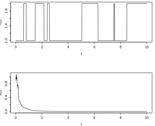
becomes τ <0.02618194. By Theorems 5.3 and 5.4, we can therefore conclude that the controlled system (75) with the control function (74) is not only exponentially stable inLq¯for
any q¯≥2 but also almost surely providedτ <0.02618194. We perform a computer simulation with τ = 0.02 and the initial vale x(0) = 1 andr(0) = 1. The sample paths of the Markov chain and the solution of the SDDE (75) are plotted in Figure 6.1. The simulation supports our theoretical results clearly.
0 2 4 6 8 10
1.0
1.4
1.8
t
r(t)
0 2 4 6 8 10
0.0
0.4
0.8
t
[image:11.612.51.299.307.509.2]x(t)
Figure 6.1: The computer simulation of the sample paths of the Markov chain and the SDDE (75) with the control function (74) and
τ = 0.02using the Euler–Maruyama method with step size10−4 .
Example 6.2: We continue with the hybrid SDE (71) but
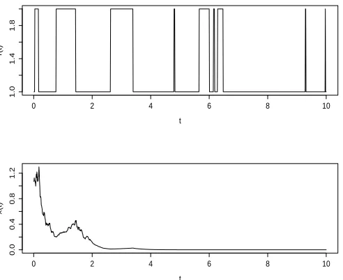
consider the case where the system is observable only in mode 1 but not in mode 2 so we could only use a feedback control in mode 1 (namely the system is not controllable or observable in mode 2 so have to set the control function to be 0 in mode 2). As the system is not controllable in mode 2, we will need to assume that the system will switch to mode 1 from 2 sufficiently faster than that from mode 1 to 2. Accordingly, instead of (73), we now assume the Markov chainr(t)has the generator
Γ =
−1 1
6 −6
. (78)
Moreover, we now design the control function
u(x,1, t) =−4x, u(x,2, t) = 0. (79)
Obviously, Assumption 2.3 is satisfied withκ= 4. The global solution of the controlled system (75) still has property (76). It is straightforward to show that, for(x, i, t)∈R×S×R+,
x[f(x, i, t) +u(x, t, i)] +1
2|g(x, t, i)|
2
≤
−2.75x4−2.75x2 ifi= 1,
−1.9375x4+ 1.0625x2 ifi= 2,
and
x[f(x, i, t) +u(x, t, i)] +q1
2|g(x, t, i)|
2
≤
−2.25x4−2.25x2 ifi= 1,
−1.8125x4+ 1.1875x2 ifi= 2.
Namely, (21) and (22) hold with
α1= 2.75, β1=−2.75, α2= 1.9375, β2= 1.0625
and
¯
α1= 2.25, β¯1=−2.25, α¯2= 1.8125, β¯2= 1.1875
respectively. Moreover,
A1=
6.5 −1 −6 3.875
and A2=
10 −1 −6 1.25
,
which are both M-matrices. That is, Condition 4.1 is satisfied. By (24), we then have
θ1= 0.2540717, θ2= 0.6514658,
¯
θ1= 0.3461538, θ¯2= 2.4615385.
The functionU defined by (25) becomes
U(x, i) =
0.2540717x2+ 0.3461538x4 if i= 1, 0.6514658x2+ 2.4615385x4 if i= 2.
By (27), we also have
LU(x, i, t)≤
−2.397394x4−x2−3.115384x6 ifi= 1,
−3.52443x4−x2−17.84615x6 ifi= 2.
Choosing γ1 = 0.1, γ2 = 0.25 and γ3 = 1, we can then
further show
LU(x, i, t) +γ1 2θi|x|+ (q1+ 1)¯θi|x|q1 2
+γ2|f(x, i, t)|2+γ3|g(x, i, t)|2
≤ −0.4741703x2−0.6736681x6. (80)
That is, Condition 5.1 is satisfied with additional γ4 =
0.4741703andγ5= 0.6736681. Consequently, Condition 5.2
becomes τ < 0.00625. By Theorems 5.3 and 5.4, we can therefore conclude that the controlled system (75) with the control function (79) is not only exponentially stable in Lq¯
0 2 4 6 8 10
1.0
1.4
1.8
t
r(t)
0 2 4 6 8 10
0.0
0.4
0.8
1.2
t
[image:12.612.52.298.71.272.2]x(t)
Figure 6.2: The computer simulation of the sample paths of the Markov chain and the SDDE (10) with the control function (78) and
τ= 0.005using the Euler–Maruyama method with step size10−4 .
VII. CONCLUSION
In this paper we have discussed the stabilisation of highly nonlinear hybrid SDEs by the feedback controls based on the discrete-time observations of the states. We pointed out that the existing results on the stabilisation of nonlinear hybrid SDEs require the coefficients of the underlying SDEs satisfy the linear growth condition. On the other hand, many hybrid SDE models in the real world do not fulfil this linear growth condition (namely, they are highly nonlinear). There is hence a need to develop a new theory on the stabilisation for the highly nonlinear SDE models. In this paper we consider a class of hybrid SDEs which are not stable but their solutions are bounded inqth moment. We then show that the controlled SDEs preserve the moment boundedness as long as the control functions satisfy the Lipschitz condition. We then show how to design the control functions more wisely so that the controlled SDEs become stable. The stability discussed in this paper include the H∞-stable in Lq¯, asymptotic stability in q¯th
moment, qth moment exponential stability and almost surely exponential stability. The key technique used is this paper is the method of Lyapunov functionals. A couple of examples and computer simulations have been used to illustrate our theory.
ACKNOWLEDGEMENTS
The authors would like to thank the National Natural Science Foundation of China (71571001), the Royal So-ciety (WM160014, Royal SoSo-ciety Wolfson Research Merit Award), the Royal Society and the Newton Fund (NA160317, Royal Society-Newton Advanced Fellowship), the EPSRC (EP/K503174/1), the Ministry of Education (MOE) of China (MS2014DHDX020) for their financial support.
REFERENCES
[1] Ahlborn, A. and Parlitz, U., Stabilizing unstable steady states using multiple delay feedback control, Physical Review Letters 93, 264101 (2004).
[2] Bahar A. and Mao X., Stochastic delay population dynamics,Journal of International Applied Math.11(4)(2004), 377–400.
[3] Cao, J., Li, H.X. and Ho, D.W.C., Synchronization criteria of Lur’s systems with time-delay feedback control,Chaos, Solitons and Fractals 23(2005) 1285–1298.
[4] Fei, W., Hu, L., Mao, X. and Shen, M., Delay dependent stability of highly nonlinear hybrid stochastic systems,Automatica82(2017), 65– 70.
[5] Feng, J., Lam, J. and Shu, Z., Stabilization of Markovian systems via probability rate synthesis and output feedback,IEEE Trans. Auto. Control55(2010), 772–777.
[6] Hu, L., Mao, X. and Shen, Y., Stability and boundedness of nonlinear hybrid stochastic differential delay equations,Systems & Control Letters 62(2013), 178–187.
[7] Ji, Y. and Chizeck, H.J., Controllability, stabilizability and continuous-time Markovian jump linear quadratic control,IEEE Trans. Automat. Control35(1990), 777–788.
[8] Kolmanovskii, V.B. and Nosov, V.R.,Stability of Functional Differential Equations, Academic Press, 1986.
[9] Ladde, G.S. and Lakshmikantham, V.,Random Differential Inequalities, Academic Press, 1980.
[10] Lewis A.L.,Option Valuation under Stochastic Volatility: with Mathe-matica Code, Finance Press, 2000.
[11] Mao, X.,Stability of Stochastic Differential Equations with Respect to Semimartingales, Longman Scientific and Technical, 1991.
[12] Mao, X., Exponential Stability of Stochastic Differential Equations, Marcel Dekker, 1994.
[13] Mao, X.,Stochastic Differential Equations and Their Applications, 2nd Edition, Chichester: Horwood Pub., 2007.
[14] Mao, X., Stability of stochastic differential equations with Markovian switching,Sto. Proc. Their Appl.79(1999), 45–67.
[15] Mao, X., Exponential stability of stochastic delay interval systems with Markovian switching,IEEE Trans. Auto. Control47(10)(2002), 1604– 1612.
[16] Mao, X., Stabilization of continuous-time hybrid stochastic differential equations by discrete-time feedback control,Automatica49(12)(2013), 3677–3681.
[17] Mao, X., Almost sure exponential stabilization by discrete-time stochas-tic feedback control, IEEE Transactions on Automatic Control 61(6)
(2016), 1619–1624.
[18] Mao, X., Liu, W., Hu, L., Luo,Q. and Lu, J., Stabilization of hybrid stochastic differential equations by feedback control based on discrete-time state observations,Systems and Control Letters73(2014), 88–95. [19] Mao, X., Lam, J. and Huang, L., Stabilisation of hybrid stochastic differential equations by delay feedback control, Systems & Control Letters57(2008), 927–935.
[20] Mao, X., Matasov, A. and Piunovskiy, A.B., Stochastic differential delay equations with Markovian switching,Bernoulli6(1)(2000), 73–90. [21] Mao, X. and Yuan, C.,Stochastic Differential Equations with Markovian
Switching, Imperial College Press, 2006.
[22] Mariton, M.,Jump Linear Systems in Automatic Control, Marcel Dekker, 1990.
[23] Mohammed, S.-E.A., Stochastic Functional Differential Equations, Longman Scientific and Technical, 1984.
[24] Pyragas, K., Control of chaos via extended delay feedback, Physics Letters A206(1995), 323–330.
[25] Qiu, Q., Liu, W., Hu, L., Mao, X. and You, S., Stabilisation of stochastic differential equations with Markovian switching by feedback control based on discrete-time state observation with a time delay, Statistics and Probability Letters115(2016), 16–26.
[26] Shaikhet, L., Stability of stochastic hereditary systems with Markov switching,Theory of Stochastic Processes2(18)(1996), 180–184. [27] Shi, P., Mahmoud, M.S., Yi, J. and Ismail, A., Worst case control of
uncertain jumping systems with multi-state and input delay information,
Information Sciences176(2006), 186–200.
[28] Sun, M., Lam, J., Xu, S. and Zou, Y., Robust exponential stabilization for Markovian jump systems with mode-dependent input delay,Automatica 43(2007), 1799–1807.
[29] Wei, G., Wang, Z., Shu, H. and Fang, J., Robust H∞ control of stochastic time-delay jumping systems with nonlinear disturbances,
[30] You, S., Liu, W., Lu, J., Mao, X. and Qiu, Q., Stabilization of hybrid systems by feedback control based on discrete-time state observations,
SIAM J. Control and Optimization53(2)(2015), 905–925.
[31] Yue, D. and Han, Q., Delay-dependent exponential stability of stochastic systems with time-varying delay, nonlinearity, and Markovian switching,
IEEE Trans. Automat. Control50(2005), 217–222.
[32] Zhang, L, Boukas, E. K. and Lam, J., Analysis and synthesis of Markov jump linear systems with time-varying delays and partially known transition probabilities,IEEE Trans. Autom. Control53(2008), 2458– 2464.
Chen Fei currently is a PhD student with the Glorious Sun School of Business and Management, Donghua University, Shanghai, China. She received the BSc degree from Fuyang Normal University, Fuyang, Anhui, China, in 2015. She was admitted to the master-and-PhD programme of applied math-ematics in Donghua University, Shanghai, China, in September 2015. Her research interests include stochastic system, financial mathematics. Miss Fei is the author of 8 research papers.
Weiyin Fei is a Professor with the School of Mathematics and Physics, Anhui Polytechnic Uni-versity, Wuhu, Anhui, China. He received the BSc degree from Anhui Normal University, Wuhu, An-hui, China, the MSc degree and the Ph.D. degree from Donghua University, Shanghai, China, in 1986, 1996, and 2002, respectively. His research interests include stochastic control, financial mathematics, and stochastic differential equation with applica-tions. Dr. Fei has authored over 180 research papers.
Xuerong Maoreceived the PhD degree from War-wick University, Coventry, U.K., in 1989. He was SERC (Science and Engineering Research Council, U.K.) Post-Doctoral Research Fellow from 1989 to 1992. Moving to Scotland, he joined the University of Strathclyde, Glasgow, U.K., as a Lecturer in 1992, was promoted to Reader in 1995, and was made Professor in 1998 which post he still holds. He was elected as a Fellow of the Royal Society of Edinburgh (FRSE) in 2008. He has authored five books and over 300 research papers. His main research interests lie in the field of stochastic analysis including stochastic stability, stabilization, control, numerical solutions and stochastic modelling in finance, economic and population systems. He is a member of the editorial boards of several international journals.
Dengfeng Xia is a Professor with the School of Mathematics and Physics, Anhui Polytechnic Uni-versity, Wuhu, Anhui, China. He received the BSc degree from Anhui Normal University, Wuhu, An-hui, China, the MSc degree from Anhui Polytechnic University, Wuhu, Anhui, China and the PhD degree from Donghua University, Shanghai, China, in 2001, 2008, and 2017, respectively. His research interests include stochastic control, financial mathematics, and stochastic differential equations and their ap-plications. Dr. Xia has authored over 30 research papers.