FCNet: A Convolutional Neural Network for Calculating Functional Connectivity from functional MRI

City, University of London Institutional Repository

Citation

:

Riaz, A., Asad, M., Al-Arid, S. M. M. R., Alonso, E., Dima, D., Corr, P. J. and

Slabaugh, G. G. (2017). FCNet: A Convolutional Neural Network for Calculating Functional

Connectivity from functional MRI. Lecture Notes in Computer Science, 10511, pp. 70-78. doi:

10.1007/978-3-319-67159-8_9

This is the accepted version of the paper.

This version of the publication may differ from the final published

version.

Permanent repository link:

http://openaccess.city.ac.uk/18045/

Link to published version

:

http://dx.doi.org/10.1007/978-3-319-67159-8_9

Copyright and reuse:

City Research Online aims to make research

outputs of City, University of London available to a wider audience.

Copyright and Moral Rights remain with the author(s) and/or copyright

holders. URLs from City Research Online may be freely distributed and

linked to.

City Research Online:

http://openaccess.city.ac.uk/

[email protected]

Calculating Functional Connectivity from

functional MRI

Atif Riaz, Muhammad Asad, S. M. Masudur Rahman Al-Arif, Eduardo Alonso, Danai Dima, Philip Corr and Greg Slabaugh

City, University of London, UK [email protected]

Abstract. Investigation of functional brain connectivity patterns us-ing functional MRI has received significant interest in the neuroimag-ing domain. Brain functional connectivity alterations have widely been exploited for diagnosis and prediction of various brain disorders. Over the last several years, the research community has made tremendous advancements in constructing brain functional connectivity from time-series functional MRI signals using computational methods. However, even modern machine learning techniques rely on conventional correla-tion and distance measures as a basic step towards the calculacorrela-tion of the functional connectivity. Such measures might not be able to capture the latent characteristics of raw time-series signals. To overcome this short-coming, we propose a novel convolutional neural network based model, FCNet, that extracts functional connectivity directly from raw fMRI time-series signals. The FCNet consists of a convolutional neural network that extracts features from time-series signals and a fully connected net-work that computes the similarity between the extracted features in a Siamese architecture. The functional connectivity computed using FCNet is combined with phenotypic information and used to classify individu-als as healthy controls or neurological disorder subjects. Experimental results on the publicly available ADHD-200 dataset demonstrate that this innovative framework can improve classification accuracy, which in-dicates that the features learnt from FCNet have superior discriminative power.

Keywords: Functional Connectivity, CNN, fMRI, Deep Learning.

1

Introduction

2 Riaz et al.

functional networks in resting state fMRI. The human brain can be viewed as a large and complicated network in which the regions are represented as nodes and their connectivity as edges of the network. FC is viewed as a pair-wise connectivity measurement which describes the strength of temporal coherence (co-activity) between the brain regions. A number of recent studies have shown FC as an important biomarker for the identification of different brain disorders like ADHD [1], schizophrenia [3] and many more.

Several methods have been developed for extracting the FC from temporal resting state fMRI data such as correlation measures [3], clustering [1] and graph measures [2]. Most of the existing techniques, including modern machine learn-ing methods like clusterlearn-ing, rely on conventional distance-based measures for calculating the strength of similarity between brain region signals. These mea-sures act as hand-crafted features towards determining the FC and, may not be able to capture the inherent characteristics of the time-series signals.

A convolutional neural network (CNN) provides a powerful deep learning model which has been shown to outperform existing hand-crafted features based methods in a number of domains like image classification, image segmentation and object recognition. The strength of a CNN comes from its representation learning capabilities, where the most discriminative features are learned during training. A CNN is composed of multiple modules, where each module learns the representation from one lower level to a higher, more abstract level. To our knowledge, CNNs have not been investigated to determine the FC of brain regions. In this work, our motivation is to construct the FC patterns from fMRI data by exploiting the representation learning capability of a CNN. Particularly, we are interested to determine if a CNN can capture the latent characteristics of the brain signals. Compared with other methods, our approach calculates the FC directly from pairs of raw time-series fMRI signals, naturally preserving the inherent characteristics of the time-series signal in the constructed FC.

For training, FCNet requires pairs of fMRI signals and a real value indicating the degree of FC. Training data is produced using a generator that selects pairs of time-series signals that are considered functionally connected, and those that are not. This data is used to train a Siamese network [4] architecture to predict FC from an input signal pair. We demonstrate the expressive power of the features extracted from the FCNet in a classification framework that classifies individuals as healthy control or disorder subjects.

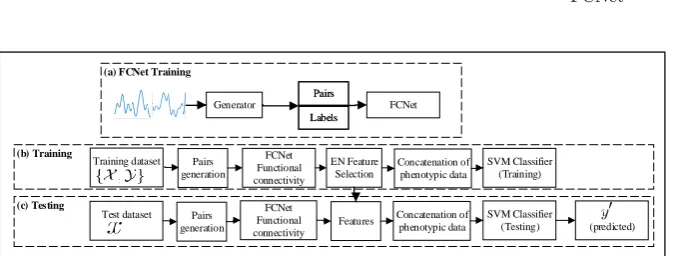
Training dataset FCNet Functional connectivity

EN Feature Selection

Concatenation of phenotypic data

SVM Classifier (Training)

Test dataset _Functional FCNet

connectivity

Features Concatenation of _{phenotypic data} SVM Classifier _{(Testing) (predicted)}

(a) FCNet Training

(b) Training

Generator FCNet

Pairs Labels Pairs Labels

(c) Testing

Pairs generation

Pairs generation

Fig. 1. Flowchart of the proposed method. In (a), FCNet is trained from the data generated by the generator. In the training pipeline (b), functional connectivity (FC) is generated through FCNet. Next, discriminant features are selected and are con-catenated with phenotypic data, then employed to train a SVM classifier. The testing pipeline is shown in (c). After FC is calculated, features are selected and concatenated with phenotypic data. A trained SVM is employed for classification.

feature map. The feature map is used to train a SVM classifier which learns to classify between healthy control and disorder subjects. Once the classification path of Fig 1b is trained, it can be used to classify test subjects as shown in Fig 1c.

The contributions of this work include: 1) a novel CNN-based deep learning model for extraction of functional connectivity from raw fMRI signals 2) a learn-able similarity measure for calculation of functional connectivity and 3) improved classification accuracy over the state-of-the-art on the ADHD-200 dataset.

2

Method

2.1 Data and preprocessing

The resting state fMRI data evaluated in this work is from the ADHD-200 con-sortium [6]. Different imaging sites contributed to the dataset. The data is com-prised of resting state functional MRI data as well as phenotypic information. The consortium has provided a training dataset, and an independent testing dataset separately for each imaging site. We have used data from three sites: NeuroImage (NI), New York University Medical Center (NYU) and Peking Uni-versity (Peking). All sites have a different number of subjects. Additionally, imaging sites have different scan parameters and equipment, which increases the complexity and diversity of the dataset. This data has been preprocessed as part

of the connectome project1_{and brain is parcellated into 90 regions using the}

au-tomated anatomical labelling atlas [7]. A more detailed description of the data and pre-processing steps appears on the connectome website. We have integrated phenotypic information of age, gender, verbal IQ, performance IQ and Full4 IQ for NYU and Peking (for NeuroImage, phenotypic information of IQs was not available).

1

4 Riaz et al.

Conv

Pool B-Norm L-ReLU

F.Conn

b) Feature extractor network

C1 C2 C3 C4 C5

C1 C2 C3 C4 C5 C

ros

s-e

nt

rop

y

los

s

F

.C

on

n

F

.C

onn

F

.C

onn +

so

ft

m

a

x

c) Similarity network

a) FCNet d) Legends

F

unc

ti

ona

l

Co

nne

c

ti

vi

ty

Fig. 2.Architecture of the FCNet. (a) FCNet with coupled feature extractor network (one network for each brain region) and the similarity network which measures the degree of similarity between the two regions. (b) The feature extractor network which includes multiple layers namely Convolutional (Conv), Batch Normalization (B-Norm), Pooling (pool), Fully Connected (F.Conn) and Leaky-ReLU (L-ReLU). (c) The simi-larity measure network. (d) Legends for feature extractor network.

2.2 Functional connectivity through FCNet

In this work, we propose a novel deep CNN for the calculation of FC. Our proposed method calculates FC directly from raw time-series signals instead of relying on conventional similarity measures like correlation or distance based measures.

FCNet is a deep-network architecture for jointly learning a feature extractor network that captures the features from the individual regional time-series signal and a learnable similarity network that calculates similarity between the pairs. The FCNet is presented in Fig 2 and individual networks are detailed below.

The feature extractor network: This network extracts features from

indi-vidual brain region time-series signals and is comprised of multiple layers that

are common in CNN models to learn abstract representations of features. Here, we use a Leaky Rectified Linear Unit (ReLU) as the non-linearity function, due to its faster convergence over ReLU [8]. The network accepts time-series signal of length 172. All pooling layers pool spatially with pool length of 2. For all convolution layers, we use kernel size of 3 and the number of filters are 32, 64,

96, 64, 64 for layersC1,C2,C3,C4,C5 respectively. The last fully connected

layer in the network has 32 nodes.

The similarity measure network: This network employs a neural network

to learn the FC between pairs of extracted features from two brain regions.

This is in contrast to conventional methods that use hand-crafted computations like correlation or distance based measures. The input to this network are the abstracted features extracted from two regions. The network computes their FC, which relates to the similarity between the two regions. The network is comprised of three fully connected layers where the last layer is connected to a softmax classifier with dense connections. Next, we describe architectural considerations and training.

same feature extraction processing. It can be realized by employing the two feature extractor networks (coupled structure) with the constraint that both networks share the same set of parameters. During the training phase, updates are applied to the shared parameters. The approach is similar to Siamese network [4] that is used to measure similarity between two images.

Data generator for training FCNet: For training FCNet, we require simi-lar (functionally connected) and dissimisimi-lar (not functionally connected) regions with corresponding labels (one and zero respectively). We develop a generator to generate pairs of brain regions using support from affinity propagation [9] clustering for labelling the training pairs. We make pairs for regions that lie in the same cluster and assign them the label one (functionally connected). For unconnected pairs (regions that are not functionally connected), we randomly pick regions that do not belong to the same cluster and label the pair zero. The procedure is detailed in Algorithm 1.

Algorithm 1: Data generation for training of the FCNet.

Input: X%Xis the subjects in training data, nReg (number of regions) = 90.

Output:(Pairs, Labels) % Pairs and Labels are used for training of FCNet.

1 for eachxinX do

2 c←cluster(x) % clustering results inc

3 count←0

4 for i←1 to nRegdo

5 for eachjin(1→nReg)such that c(xi) = c(xj) andi6=jdo

6 AddToPairs((xi,xj), Pairs)

7 AddToLabels(1, Labels)

8 count←count + 1

9 end

10 fork←1 to count do

11 r←RandomSelectRegion(x) such that c(xi)6= c(r)

12 AddToPairs((xi,r), Pairs)

13 AddToLabels(0, Labels)

14 end

15 end

16 end

17 return (Pairs,Labels)

Training of FCNet: FCNet is trained on pair-wise signals with labels gener-ated from the generator as described above. The FCNet is trained end-to-end using a coupled architecture minimizing the cross-entropy loss

Lf c=−

1

n

n

X

1

[yilog( ˆyi) + (1−yi)log(1−yˆi)], (1)

where n is the number of training samples, yi is the label of pairs (1 for

func-tionally connected and 0 for unconnected regions) and ˆyi is the prediction by

6 Riaz et al.

Table 1.Comparison of FCNet with the average results of competition teams, highest accuracy achieved for individual site, correlation based FC and state-of-the-art clus-tering based FC results [1]. The highest accuracy for NI was not quoted by [10].

NI Peking NYU Average accuracy [6] 56.9% 51.0% 35.1% Highest accuracy [10] – 58% 56% Clustering method [1] 44% 65% 61% Correlation 52.0 % 52.9% 56.1% Proposed method 64.0% 68.6% 63.4%

To evaluate FC through the FCNet, regions belonging to each subject are grouped into pairs (for 90 regions belonging to a subject 4005 unique pairs are created). The pairs are passed to the trained FCNet, which computes FC for each pair.

2.3 Feature Selection and Classification

The FC of a subject may contain highly correlated features. We investigate Elas-tic Net (EN) based feature selection [5] for extracting discriminant features. EN

combines the L1 penalty to enable variable selection and continuous shrinkage,

and theL2 penalty to encourage grouped selection of features. Ifyis the label

vector for subjects yi(l1, l2, ...ln) andX ={F C1, F C2, ...F Cn} represents the

functional connectivity of subjects, we minimize the cost function

Len(λ1, λ2, β) = (||y−Xβ||)2+λ1(||β||)1+λ2||β||2, (2)

where λ1 and λ2 are weights of the terms forming the penalty function, and

β coefficients are calculated through model fitting. The features with non zero

β coefficients relating to minimum cross validation error are extracted. Similar

to [1], phenotypic information of the subjects are concatenated with the EN based selected features to construct a combined feature set for classification.

The final step in the proposed framework is classification where a support vector machine (SVM) classifier is utilized to evaluate the discriminative ability of the selected features.

3

Experiments and Results

The proposed framework is evaluated on a dataset provided by the ADHD-200 consortium, and contains four categories of subjects: controls, ADHD com-bined, ADHD hyperactive-impulsive and ADHD inattentive. Here we combine all ADHD subtypes in one category since we want to investigate classification between healthy control and ADHD.

provided for each individual site, and results are presented in Table 1. The results show that our method outperforms the average accuracy results of competition teams (data from the competition website), highest accuracy for any individual site (from [10]) and correlation-based FC results. For correlation based results, FC is calculated through correlation and the rest of processing pipeline is same as our method. It is worth noting that the parameters of our framework are held constant for all the imaging datasets. Our method also performs well in comparison with a state-of-the-art clustering based FC technique [1]. In order to compare with the related work [1] that employed phenotypic information, we compare and present the results in Table 2, which shows that our method performs well in all of the three imaging sites. Finally, in order to study the FC differences between the healthy control group and the ADHD group, we visualize their respective FC patterns using the Peking dataset and present the results in Fig 3. The results show that in ADHD, the temporal lobe functional connectivity is reduced compared to healthy controls.

(L)  H ip p o (R)  H ipp o (L)  Pa. G (R)  Pa.G (L) 

Am ygd ala

(R) A mygda

la (L) S .T.P (R) S .T.P (L) M .T.P (R) M .T.P (L) O .C (R) O .C (L) C .N (R) C.N

(L) Pu tamen (R) Putamen

(L) G.P (R) G.P

(L) Thalamus (R) Thalamus (L) C.S (R) C.S (L) Cu (R) Cu (L) L.G (R) L.G (L) S.O (R) S.O (L) M.O (R) M_.O (L) I.O (R) _I.O (L ) F.G (R_) F .G (L ) S .F.G­Dl (R ) S .F.G ­Dl (L ) S_.F .G ­O (R ) S_.F .G ­O (L ) M .F_.G ­L (R ) M .F_.G ­L (L ) M_.F .G ­O (R ) M_.F .G ­O (L ) I .F_.G ­O r (R ) I .F .G ­O r (L ) T ri (R ) T ri (L ) I .F .G ­O (R ) I.F .G ­O (L ) S .F .G ­M e (R ) S .F .G ­M e (L ) S .F .G ­M eO (R ) S .F .G ­M eO (L ) G .R (R ) G .R (L ) A .C .G (R ) A .C .G (L ) R .O (R)  R.O (L)  Ins ula (R)  In sula (L)  T. T.G (R ) T .T .G (L ) S .T .G (R ) S .T .G (L ) M .T .G (R ) M .T .G (L ) I .T .G (R ) I .T .G P.G (L ) P.G (R ) (L ) S .M .A (R ) S .M .A (L ) M .C (R ) M

.C .C) P(L .G .C) P(R

.G ) P(L o.G ) P(R

o.G ) S(L

.P .L (R ) S .P .L (L ) I .P .L (R ) I .P .L (L ) S l.G (R ) S l.G (L )  A .G (R )  A .G (L )  P re cu n eu s (R )  P re cu n eu s (L )  P a. L (R )  P a. L Medial Te mporal Su_bc ort_ica l O cc ip ita l Fro nta l Te m po ra l Parie tal (p re) m otor

(a) FC patterns of the healthy control group.

(L)  H ip p o (R)  H ipp o (L)  Pa. G (R) 

Pa.G (L) 

Am ygd ala

(R) A mygda

la (L) S .T.P (R) S .T.P (L) M .T.P (R) M .T.P (L) O .C (R) O .C (L) C .N (R) C.N

(L) Pu tamen (R) Putamen

(L) G.P (R) G.P

(L) Thalamus (R) Thalamus (L) C.S (R) C.S (L) Cu (R) Cu (L) L.G (R) L.G (L) S.O (R) S.O (L) M.O (R) M_.O (L) I.O (R) _I.O (L ) F.G (R_) F .G (L ) S .F.G­Dl (R ) S .F.G ­Dl (L ) S_.F .G ­O (R ) S_.F .G ­O (L ) M .F_.G ­L (R ) M .F_.G ­L (L ) M_.F .G ­O (R ) M_.F .G ­O (L ) I .F_.G ­O r (R ) I .F .G ­O r (L ) T ri (R ) T ri (L ) I .F .G ­O (R ) I.F .G ­O (L ) S .F .G ­M e (R ) S .F .G ­M e (L ) S .F .G ­M eO (R ) S .F .G ­M eO (L ) G .R (R ) G .R (L ) A .C .G (R ) A .C .G (L ) R .O (R)  R.O (L)  Ins ula (R)  In sula (L)  T. T.G (R ) T .T .G (L ) S .T .G (R ) S .T .G (L ) M .T .G (R ) M .T .G (L ) I .T .G (R ) I .T .G P.G (L ) P.G (R ) (L ) S .M .A (R ) S .M .A (L ) M .C (R ) M

.C .C) P(L .G .C) P(R

.G ) P(L o.G ) P(R

o.G ) S(L

.P .L (R ) S .P .L (L ) I .P .L (R ) I .P .L (L ) S l.G (R ) S l.G (L )  A .G (R )  A .G (L )  P re cu n eu s (R )  P re cu n eu s (L )  P a. L (R )  P a. L Medial Te mporal Su_bc ort_ica l O cc ip ita l Fro nta l Te m po ra l Parie tal (p re) m otor

(b) FC patterns of the ADHD group.

Fig. 3.Comparison of mean functional connectivity (FC) of healthy control group (a) and ADHD group (b) for the Peking dataset. For the sake of clarity, only the top 200 connections (based upon their connectivity strength) from both groups are presented. The FC patterns show alterations. The temporal lobe FC patterns are altered the most with a decrease of 15% FC patterns in the ADHD group. The inter-temporal lobe FC patterns are reduced from 22.7% (healthy group) to 7.7% (ADHD group).

4

Conclusion

8 Riaz et al.

Table 2. Comparison of proposed method with the state-of-the-art results [1]. The results suggest that the FCNet outperforms the state-of-the-art classification accuracy.

Phenotypic

information Method NI Peking NYU

Not used Clustering method [1] 44% 58.8% 24.3% Proposed method 60.0% 62.7% 58.5% Used Clustering method [1] – 65% 61%

Proposed method 64.0% 68.6% 63.4%

from the raw time-series signals and a learnable similarity measure network that calculates the similarity between regions. The FCNet is an end-to-end trainable network. After calculating functional connectivity, elastic net is applied to se-lect discriminant features. Finally, a support vector machine classifier is applied to evaluate the classification results. Experimental results on the ADHD-200 dataset demonstrate promising performance with our method.

References

1. Riaz, A., Alonso, E., Slabaugh, G.: Phenotypic Integrated Framework for Classi-fication of ADHD using fMRI. In: International Conference Image Analysis and Recognition, Springer (2016) 217–225

2. Dey, S., Rao, A.R., Shah, M.: Attributed graph distance measure for automatic detection of attention deficit hyperactive disordered subjects. Frontiers in Neural Circuits8(2014)

3. Kim, J., Calhoun, V.D., Shim, E., Lee, J.H.: Deep neural network with weight spar-sity control and pre-training extracts hierarchical features and enhances classifica-tion performance: Evidence from whole-brain resting-state funcclassifica-tional connectivity patterns of schizophrenia. NeuroImage124(2016) 127–146

4. Bromley, J., Guyon, I., LeCun, Y., S¨ackinger, E., Shah, R.: Signature Verification using a “Siamese” Time Delay Neural Network. In: Advances in Neural Information Processing Systems. (1994) 737–744

5. Zou, H., Hastie, T.: Regularization and variable selection via the elastic net. Jour-nal of the Royal Statistical Society: Series B (Statistical Methodology)67(2) (2005) 301–320

6. ADHD-200. http://fcon_1000.projects.nitrc.org/indi/adhd200/

7. Tzourio-Mazoyer, N., Landeau, B., Papathanassiou, D., Crivello, F., Etard, O., Delcroix, N., Mazoyer, B., Joliot, M.: Automated anatomical labeling of activations in SPM using a macroscopic anatomical parcellation of the MNI MRI single-subject brain. NeuroImage15(1) (2002) 273–289

8. Maas, A.L., Hannun, A.Y., Ng, A.Y.: Rectifier nonlinearities improve neural net-work acoustic models. In: International Conference on Machine Learning. Vol-ume 30. (2013)

9. Frey, B.J., Dueck, D.: Clustering by passing messages between data points. Science

315(5814) (2007) 972–976