HARD: Hybrid Adaptive Resource Discovery for Jungle Computing

City, University of London Institutional Repository

Citation: Zarrin, J., Aguiar, R. L. and Barraca, J. P. (2017). HARD: Hybrid Adaptive

Resource Discovery for Jungle Computing. Journal of Network and Computer Applications,

90, pp. 42-73. doi: 10.1016/j.jnca.2017.04.014

This is the accepted version of the paper.

This version of the publication may differ from the final published

version.

Permanent repository link: http://openaccess.city.ac.uk/18146/

Link to published version: http://dx.doi.org/10.1016/j.jnca.2017.04.014

Copyright and reuse: City Research Online aims to make research

outputs of City, University of London available to a wider audience.

Copyright and Moral Rights remain with the author(s) and/or copyright

holders. URLs from City Research Online may be freely distributed and

linked to.

City Research Online:

http://openaccess.city.ac.uk/

[email protected]

HARD: Hybrid Adaptive Resource Discovery for Jungle Computing

Javad Zarrin, Rui L. Aguiar, Jo˜ao Paulo Barraca

Javad Zarrin{[email protected]}Instituto de Telecomunica¸c˜oes - Aveiro. Rui L. Aguiar{[email protected]}Universidade de Aveiro, Portugal. Jo˜ao Paulo Barraca{[email protected]}Universidade de Aveiro, Portugal.

Abstract

In recent years, Jungle Computing has emerged as a distributed computing paradigm based on simultaneous combination of various hierarchical and distributed computing environments which are composed by large number of heterogeneous resources. In such a computing environment, the resources and the underlying computation and communication infrastructures are highly-hierarchical

and heterogeneous. This creates a lot of difficulty and complexity for finding the proper resources in a precise way in order to run

a particular job on the system efficiently. This paper proposes Hybrid Adaptive Resource Discovery (HARD), a novel efficient

and highly scalable resource-discovery approach which is built upon a virtual hierarchical overlay based on self-organization and self-adaptation of processing resources in the system, where the computing resources are organized into distributed hierarchies according to a proposed hierarchical multi-layered resource description model. The proposed approach supports distributed query processing within and across hierarchical layers by deploying various distributed resource discovery services and functionalities in the

system which are implemented using different adapted algorithms and mechanisms in each level of hierarchy. The proposed approach

addresses the requirements for resource discovery in Jungle Computing environments such as high-hierarchy, high-heterogeneity,

high-scalability and dynamicity. Simulation results show significant scalability and efficiency of the proposed approach over highly

heterogeneous, hierarchical and dynamic computing environments.

Keywords: distributed operation systems, many-core systems, P2P, resource management, grid computing, DHT

Acronyms

vnodevirtual node.

ANaggregate-node.

BRW2 a 2-layered hybrid broad-cast and full random-walk

based discovery.

DHTdistributed hash table.

DOSdistributed operation system.

DPTdistributed probability table.

FRW2a 2-layered hybrid DHT and full random-walk based

discovery.

HARDHybrid Adaptive Resource Discovery.

HARD2a 2-layered instantiation of HARD.

HARD3a 3-layered instantiation of HARD.

JCSJungle Computing System.

LNleaf-node.

PRW2 a 2-layered hybrid DHT, learning-based and partial

random-walk based discovery.

QMSQuery Management Service.

QREGQuery Registry.

QROUTQuery Router.

RPResource Information Provider.

RRResource Requester.

SNsuper-node.

SoRSource of Resource.

SQMSSuper Query Management Service.

1. Introduction

Large scale distributed computing technologies such as Cloud, Grid, Cluster and High Performance Computing (HPC) super-computers are evolving with the revolutionary emergence of many-core designs (e.g. GPU, CPUs on single die, supercom-puters on chip, etc.) and significant advances in networking and interconnect solutions [1]. This has led to increase complex-ity on the integration of such diverse computing environments, infrastructures, platforms and technologies. Moreover, data dis-tribution, hardware availability, software heterogeneity, and also the sheer size of scientific problems, commonly force scientists to resort to Jungle Computing instead of traditional supercom-puters and clusters. Jungle Computing (i.e., leveraging multiple computing platforms simultaneously) is a recent distributed com-puting paradigm based on concurrent combination of various hierarchical and distributed computing environments with large number of heterogeneous resources [1–8]) .

In fact, integration of different resources would be necessary

specially when no single resource is available that its computa-tion of capacity can meet the computacomputa-tion requirements, or if

different parts of the computation have different computational

requirements. Furthermore, for large number of users and ap-plications, combination of multiple computing environments with various types of resources leads to achieve high peak per-formance by potentially accessing a many diverse collection of

resources while it is cost efficient. There exist many types of

that can be efficiently integrated as so-called Compute Jungles at a low cost. However, high heterogeneity (in terms of hardware, resources, connectivities and platforms) and complex hierarchi-cal design of Compute Jungles make them more complex to be efficiently used by scientists.

In a large scale system, where we have a pool of distinct processors, the enabling technology for enhancing the whole throughput of the system is resource sharing. Depending on the

computing environment, resource sharing might lead to diff

er-ent issues such as resource allocation, resource provisioning, scheduling, resource description, resource discovery and

pro-cess migration. Among them, scalable and efficient resource

discovery is one of the most challenging issues, particularly for decentralized systems (i.e., resources should be found before we can share them). This is be even more critical for future large scale computing environments (e.g., future Cloud, Grid, HPC and Cluster) and also Jungle Computing Systems (JCSs) due to the disparate requirements of these computing environments such as high heterogeneity, high hierarchy and high dynamicity . Resource discovery in JCS can be characterized as a highly adap-tive approach (considering the diversity of hardwares, platforms and computing infrastructures) to instantaneously find the most appropriate available set of resources (i.e., computing resources, like as processing cores) for the user applications in the system with minimum cost of communication and computation (i.e., in

terms of network latency, network traffic, discovery load, etc.),

based on a specific set of computational and communicational requirements for each application or application segments. This has to be achieved in a way that the static and dynamic proper-ties of resources, as well as their interconnected and aggregated characteristics, could be qualified according to the query re-quirements. Moreover due to the intrinsic complexity of JCS environments, high performance applications then require that resource discovery supports some other important features such as proximity-awareness (i.e., the , the discovered resources must be close as much as possible) and querying flexibility (in terms of complex querying such as multidimensional querying).

This paper proposes Hybrid Adaptive Resource Discovery

(HARD), an efficient and highly scalable resource-discovery

approach which deals with the aforementioned resource discov-ery requirements, applicable to large heterogeneous and highly dynamic distributed environment of JCS . HARD is based on self-configuration and self-adaptation of processing resources in the system, where the computing resources are organized into distributed hierarchies according to a proposed hierarchical resource description model (i.e., multi-layered resource

descrip-tion). Moreover, different algorithms and adapted mechanisms

(such as distributed hash tables, distributed probability tables

and any-casting) are implemented at different layers in order

to efficiently guide queries to proper resources within the

spe-cific features of that layer (e.g. leaf-node, aggregate-node and super-node layers).

This work was developed under the framework of the S[o]OS (Service-oriented Operating System) project [9–17], European research project aiming to generate a reference addressing ar-chitectures for future very large scale distributed infrastructures. The remainder of the paper is structured as follows. In the next

section, we discuss general requirements and design principles for our work including our hierarchical resource description model. The details of system architecture and HARD are pre-sented in Section III. Section IV presents our algorithms for

querying in different layers. Simulation settings and

experi-mental results for the proposed resource discovery are given in Section V. The resource discovery approaches for distributed computing environments in the literature are reviewed and fronted in Section VI and finally Section VII presents our con-clusion and future work.

2. Motivation

The motivation behind this work is to propose a resource discovery solution for very large scale distributed systems with respect to the requirements of future large dimensions, many-core enabled, computing systems. Our desired target computing environment can be described as a large scale (ideally, Internet scale), chaotic environment (jungle) of (heterogeneous) process-ing cores, connected through high speed networks and inter-connects and widely distributed across the system. Resource discovery requirements for such future systems are beyond the techniques used in today’s Grids, Clouds and HPC clusters. We were inspired by the concept of “Jungle Computing”, introduced in the recent years [1–8], and accordingly, we can envision that most of requirements for Jungle can be applied for future com-puting systems. In fact, two important features of such future environments are: first, heterogeneity of resources; and, second, very large number of resources. With respect to these features, the main objective of this work is to provide a scalable solution. Current computing systems such as Cloud, HPC and Cluster

are generally based on a centralized/hierarchical architecture,

leading to the use of centralized resource discovery to respond to user requests. For example, when a request for resources arrives at a HPC cluster-head or a Cloud service provider in the front-end, the resources required can be discovered (allocated or provisioned) by searching in a specified pool of resources or in a back-end data-center where the number and type of resources are known beforehand (this may not be necessarily true in Clouds). For such environments, resource discovery based on a centralized architecture could become an easy task. And, in fact, instead of discovery problem, the resource scheduling issues are dominant.

However, centralized approaches are not scalable and they can not cope with the requirements of future computing systems (future Clouds and HPCs) due to their well-known limitations

(bottleneck/congestion issues). This also becomes more

Unlike the aforementioned computing systems, decentralized

resource discovery approaches are mostly intended/desired for

Grids. However, these approaches generally work at task level (due to the Grid nature) in which parallelism of independent tasks is exploited. This makes current Grid discovery methods inadequate to deal with the many-core nature of future

comput-ing (in terms of efficient satisfaction of all query constraints)

[18,19], due to the lack of support for thread-level discovery. On the other hand, Operating Systems can perform resource allocation in instruction-level. This provides motivation to go beyond the Grids through the concept of distributed operation systems (DOSs), capable to run on the aforementioned future computing systems. For such DOSs, we used as reference the systems envisaged in the S[o]OS [9–17] project, and propose a thread-level resource discovery approach which works in a fully decentralized, self-determining and autonomous fashion, being

able to automatically and efficiently alter any P2P-like

underly-ing computunderly-ing system to a hierarchically structured overly. With respect to decentralization and referring to our target computing environment, described above, it is not guaranteed for a pro-cessor to have information about all other propro-cessors (or even one processor) in the system. In order to address such potential issues, we designed our discovery approach with having this assumption that all processors in the system have equal infor-mation initially (and in fact, each processor only knows about itself and its connection gates), leading us to the area of P2P computing.

3. Design Principles

For uniformity of discussion, for JCS environments we will address all kind of control systems as DOSs, although their

realization may be quite different (depending on the specific

large scale computing technology under discussion).

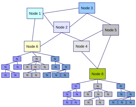
The general architecture design of a JCS environment can be illustrated as a set of distributed hierarchies like the one shown

in the Figure1. Depending on the level of hierarchies in the

architecture and the other designing aspects of a DOS , we may

define Control entities in different levels. For instance, as it is

discussed in [9], we can describe the entities of Main-Control (i.e., DOS main-kernel), Micro-Control (i.e., DOS micro-kernel) and Nano-Control (i.e., DOS nano-kernel), which are providing either maximal, moderate or minimal amount of capabilities, functionalites and services in the system. These control entities

may differ in terms of service types which they can

dynami-cally instantiate on demand. The instances of these entities are positioned in the system in a way to map the structure of the un-derlying distributed hierarchies (e.g., deploying the main-control instances in the hierarchies head-nodes and the nano-control in-stances in the leaf-nodes).

3.1. Assumptions and Definitions

HARD is based on methods and techniques to distribute re-source information, update and exchange rere-source data and query and search space exploration, specially when considering

Figure 1: An example of distributed hierarchical architectures.

the particular challenges and requirements of distributed oper-ating systems. In order to create such solution, we impose the following assumptions on the design process:

• We assume that each single resource (i.e., single core) has

its own unique ID (e.g., IP, network-ID, Chip-ID, processor-ID) which can specify its address in the entire system. Ad-dressing information can potentially be provided by the operating system or other system component, and is out of scope in this paper.

• We assume that the target computing environment can

be-have like a P2P distributed environment containing large number of peers (i.e., resource or computing entities) where each peer only knows about itself and its connection gates.

The proposed discovery approach is based on a hybrid virtual overlay network, which will be constructed automatically over the underlying physical network. This virtual overlay contains virtual-nodes that are organized in distributed hierarchies. In this work, we present a 3-layered instantiation of HARD (HARD3), which proposes two levels of resource discovery services (i.e., types of resource discovery components): Resource Requester (RR) and Resource Information Provider (RP). RP services also includes Query Management Service (QMS) and Super Query Management Service (SQMS). We will discuss these services in

more detail later in Section4.1. We will also use the following

definitions:

• We define the notion of a “virtual node (vnode)” as a group

of homogeneous resources, which are not necessarily posi-tioned on a common physical node (e.g., a CPU). Rather they are positioned within a common vicinity that is de-scribed by parameters such as number of hops or

intercon-nect latency (i.e., resources are grouped withinvnodes by

be used instead ofvnodewhich also has the same mean-ing with more emphasizmean-ing on the resource-supply-quality aspects such as SoR’s stability or SoR’s strength.

• Everyvnodeis automatically assigned a module-role (i.e.,

vnode-type) in a self-organized and distributed fashion. The

module-role defines the specific vnode’s role to play in

the overall distributed resource discovery operations. We

discuss module-roles with more detail in Section4.1.

• The term “cell” is used to denote a group ofvnodes which

are sharing a common SQMS-ID and the term ”mini-cell”

is used to refer a group ofvnodes with a common QMS-ID.

• For better illustration and evaluation of our approach, we

use throughout the paper the notion of “resource” to refer to “computational resource” (i.e., physical processing cores) and we discuss resource discovery mostly from the point of view of computational capacity. Nevertheless, HARD is fully generic, and applicable to other types of resources (e.g. storage and networking resources).

HARD3 is implemented as part of the S[o]OS concept [9], which in itself is an example of a DOS. Each DOS kernel, regard-less of its level (i.e Main, Micro, Nano, etc.), provides support for a single RR service. Furthermore, the kernels depending on the level which are positioned in the hierarchy provide support for other types of resource discovery services such as QMS and SQMS (e.g., main-kernels or micro-kernels may provide SQMS or QMS services). We must note that it may be possible that a kernel simultaneously provides either one, two or all of these discovery services. For example, the kernels in the top level of hierarchy support all kind of discovery services.

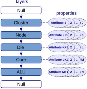
3.2. Resource Description

Resource discovery for the DOS running on the many-core enabled JCS hardware infrastructures requires a scalable and powerful hardware resource description model. In fact, it must deal with two important aspects of resource description: captur-ing static and dynamic capabilities of hardware resources; and making distribution of hardware information scalable. Consid-ering the aforementioned aspects, we introduce a hierarchical model for dynamic resource description focusing on making the distribution of resource information scalable and able to balance load. It is based in a modular information model that can

encap-sulate, interface and aggregate the different types of processing

hardware information in a hierarchical fashion.

We aim to abstract the characteristics and behavior of under-lying hardware infrastructures in a way that both computational and communicational system properties are well represented to provide a close estimation of the real system, while avoiding to describe the hardware at the cycle-accurate level. The descrip-tion model only focuses on capturing the necessary informadescrip-tion

that will aid different algorithms along the lines of resource

discovery.

The depth of hierarchy (i.e., number of layers in resource description model) and the definition of each layer might range from very high level (e.g. super clusters, clusters) to very low

level (e.g. processing core, ALUs) depending on architecture designing aspects. The layering is performed by partitioning

the total number ofnpeers (i.e., resources) in the system into

cdisjoint cells of peers (i.e.,cis the number of hierarchies in

the distributed environment), in the way to ensure that peers in the same layer of each cell are similar to one another in some predefined and inherited attributes. Each layer has two unique related layers: parent layer and child layer. A layer can be either a blank (null) layer with completely no information (definition) or it can be an identifiable layer with a deterministic definition. Furthermore, the properties of the peers in the upper layers are

also inherited by the peers in the lower layers (see Figure2).

Figure 2: An example of description of resources in hierarchical layers

We must note that the definition of a ”resource” (i.e., comput-ing resource) in HARD might be highly variable dependcomput-ing on the levels of the described hierarchy. In fact, HARD refers to a single resource as a representation of any individual peers, be-longing to the lowest level of the resource description hierarchy. For example, we can define the ALU layer (i.e., the processing unit or micro-architecture layer) to describe the properties of computing resources in a low level layer with very detail infor-mation. The ALU layer also can describe how the ALUs of a processor (CPU or core) gains access to data. In other words it has to decide on the number of the words to be used per cycle, how wide the words should be and whether the word sizes are configurable or not, etc. A HARD resource can represents either a single ALU or a single core if the description model describes either the ALU layer or the Core layer accordingly as the lowest level of the hierarchy. Note that the granularity of the hierarchies will depend on the usage intended for JCS.

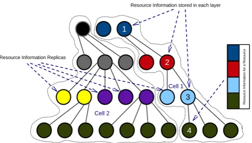
According to the proposed resource description we do not need to store locally all the information of a specific resource. The common resource information in each layer, instead of being repeated in all the peers in a local cell, is just maintained in a

certain number of peers which are offering resource information

services to other nodes in the group or network. Figure3depicts

the distribution of resource information in two individual cells (group of resources) where due to hierarchy, each cell in each layer stores the common information of the members in the lower layers in certain peers which are providing the information services to the others.

architec-Figure 3: Distribution of resource information in a four-layers-hierarchy with 2 cells

ture and capabilities (i.e., hardware description) available across

computing nodes (for efficient code/application distribution) in

heterogeneous large-scale dynamic environments, we need to

categorize information relevant at the different hierarchies. As

the systems are potentially highly dynamic (ephemeral connec-tivity of mobile devices), capability information might have to be transmitted frequently, imposing the need to minimize overhead of hardware resource description (or capability information) ex-change. For this purpose, a hierarchical capability information encoding makes sense, as we can reduce capability information being transmitted to that which is relevant for each specific level in the hierarchy.

We must also note that, one of the primary performance aspect for any hardware description model is related to all forms of communication and data exchange between any two endpoints. It is thereby irrelevant whether the communication takes place between two code instances (threads), residing on two individ-ual single cores, or between a code instance and a storage unit (i.e., between a single core processing unit and a memory unit such as cache or main memory). In all cases, the limiting per-formance factor is given by the hardware characteristics of the

interconnects affected. Furthermore, the degree and types of

communication potentially taking place in a system and for an application execution are manifold, ranging from register ac-cess over shared data to explicit communication. In all these operations, it is possible that the nodes (individual computing hardwares) in the system, require to exchange their capability information (i.e., resource description). To do this, due to the

potential network overhead and traffic, the data size (description

size) and the transaction frequency of the description must be reduced as much as possible.

In this paper, for the sake of simplicity in implementation and evaluation of our work, we assume that our description model contains three levels (layers) of the hierarchy, and we refer to this implementation as HARD3. However, depending on the system design concerns and the level of required hardware information details, further layers can also be defined (as described in Figure 2). The following part describes the main lines of information

gathered in different layers of our devised resource description

model, as implemented in this work:

• Layer 1: Core Layer (Inter-Core Level) describes the

in-dividual characteristics of the processing cores as well as cache hierarchies, the connections between processing

units, and memory layout/segmentation. Examples of

at-tribute definitions in this layer include cache size, cache associativity, cache latency, memory latency, number of Data-PU channels, number of Instruction-PU channels, vec-tor length, core clock rate (CCR), L1 cache size (L1S), L2 cache size (L2S), number of ALUs (NA), etc.

• Layer 2: Die Layer (Inter-Chip Level) describes the overall

properties and behavior of the processing dies (e.g. CPU, GPU, etc.) as well as the interconnection network and

topol-ogy of the different CPUs to form a many-core machine.

Examples of attribute definitions in this layer include BUS frequency, memory bandwidth, memory latency, cache co-herence, ISA, micro architecture, interconnection network (INT), size of processor address BUS, processor class, pro-cessor type (PT), number of cores (NC), etc.

• Layer 3: Node Layer (Inter-Board Level) describes the

overall dynamic and static characteristics of the network nodes containing multiple dies with multiple cores per die. It also describes network topology and inter-nodes commu-nication properties. Examples of attribute definitions in this layer include window size, total number of cores (TNC), memory size (MS), Die count (DC), network bandwidth (NB), network latency, etc.

3.3. Syntaxes and Description Examples

The proposed description model can flexibly describe vari-ous ”systems” and ”queries”, ranging from very simple to very complex, while enabling scalable distribution of the resource information across the system. Here, we briefly discuss the fea-tures and the syntax of our description language for describing attributes, layers, queries and systems. We store the definitions of layers and attributes in files with extension ”.def”. We also store the descriptions of queries and systems into files with extension ”.des”.

3.3.1. Defining Layers and Attributes

Grammar1presents the syntax, by Backus-Naur Form (BNF)

grammar, for defining layers and attributes using our resource description language. All definitions required for a system de-sign, including layers and attributes, must priorly be declared

using thedefinitionrule in a .def file. This can be done by

us-ing keyworddef, followed by anidentifier and sequences of

layer-definitions. The syntax also supports two other alternative expressions in order to provide capability to define attributes

in-dependent oflayer-definitions. These expressions include either

specified in the query. They are specified by using keyword attributesat the beginning of a block.

<Definition> ::= def <Identifier> <LayerDefinitionList> end | def <Identifier> <LayerDefinitionList> <OtherAttributes> end | def <Identifier> <OtherAttributes> end

<OtherAttributes> ::= attributes <AttributeDefinitionList> end <LayerDefinitionList> := <LayerDefinition>

| <LayerDefinition> <LayerDefinitionList> <LayerDefinition> ::= layer <Identifier> static : <

AttributeDefinitionList> dynamic : <AttributeDefinitionList> end | layer <Identifier> <Options> <AttributeDefinitionList> end | layer <Identifier> <AttributeDefinitionList> end <AttributeDefinitionList> ::= <AttributeDefinition>

| <AttributeDefinition> , <AttributeDefinitionList> <AttributeDefinition> ::= [<AttributeID>] <Identifier> <

AttributeDescription> : <AttributeType> <Options> ::= dynamic | static

<AttributeType> ::= <Number> | byte | <BitString>

<BitString> ::= bitstring (<Number>, value) { <ValueDefinitionList> } | bitstring (<Number>, bit) { <BitDefinitionList> } <ValueDefinitionList> ::= <ValueDefinition>

| <ValueDefinition> , <ValueDefinitionList>

<BitDefinitionList> ::= <BitDefinition> | <BitDefinition> , < BitDefinitionList>

<ValueDefinition> ::= <Value> = <ValueDescription> | < ValueDescription> = <Value>

<BitDefinition>::= bit<Number> = <BitDescription> |<BitDescription> = bit<Number>

Grammar 1: The grammar to define layers and attributes in .def files

The keywordlayeris used to define a layer. Alayer-definition

consists of a list ofattribute-definitionswhere each

attribute-definitionindividually defines a built-in attribute for its

corre-sponding layer. Anattribute-definitioncan be specified by an

uniqueattribute-idfollowed by an identifier, a short description

of the attribute and the type of attribute. In addition, we can specify whether the defined attributes are static or dynamic, by

using keywords staticanddynamicin the body of the

layer-definitionand before defining each set of attributes (attributes are specified as static by default). Static attributes (e.g., CPU type) represent attributes that do not change at runtime. In con-trary, dynamic attributes (e.g., CPU load) will potentially change

at runtime. The type of each attribute can benumber(positive

integer),byteorbitstring. Abitstringis defined as a sequence

of zero or more bits, by using keyword bitstringfollowed by

a number in parentheses, where the number indicates the

num-ber of bits required. The typebitstringis useful to efficiently

represents attributes which their values can be either one of

multiple fixed-choices (i.e.,bitstring(number,value)) or a

com-bination of multiple fixed-choices (i.e.,bitstring(number,bit)).

For example we can specify the type of AF attribute (ALU

Functionalities) for each core asbitstring(11,bit), where each

bit in the binary string (with length=11 bits) indicates whether

a specific functionality is supported or not (e.g., ”And”=bit0,

”OR”=bit1, ”Not”=bit2, ”XOR”=bit3, ”Add”=bit4, ”Sub”=bit5,

”Mul”=bit6, ”Div”=bit7,”ShiftL”=bit8, ”ShiftR”=bit9,

”Ro-tate”=bit10). Another example would be the attribute INT

which describes the topology of interconnection network for

a processor. We can define the type of this attribute as

bit-string(3,value)where each possible value of the attribute can

represents a specific topology as listed as following: ”Bus”=0,

”Ring”=1, ”NOC”=2, ”Crossbar”=3, ”PointToPoint”=4,

”Hier-archicalNOC”=5, ”Others”=6.

Listing 2presents a description example, using Grammar

1, which includes definitions of 3 layers: Layer1, Layer2 and Layer3. Each layer consists of definition of 2 to 4 individual built-in attributes. Each attribute definition includes attribute-id, attribute-name, attribute-description and attribute type. The description specifies a set of pre-defined potential values for the bitstring-type attributes (PT and ISA). The code also includes the

definition of 4 independent attributes at the end of thedef-block

which define a set of inter-node and inter-group communication attributes to describe queries.

def"in-a.def"

layerLayer1

[1] CCR"Core Clock Rate by MHz" :number, [2] L1S"L1 Cache Size by KB" :number, [3] L1L"L1 Latency by ns" :number, [4] L2S"L2 Cache Size by KB" :number end

layerLayer2

[5] PT "Processor Type":bitstring(2,value) {"CPU"=0, "GPU"=1,

"FPGA"=2,"Others"=3} ,

[6] ISA"Instruction Set Architecture" :bitstring(3,value) {" X86"=0,"SPARC"=1,"ARM"=2,"XCORE"=3, "RISC"=4,"CISC"=5,

"Legacy"=6, "Others"=7}

end

layerLayer3

[7] MS "Memory Size by MB":number, [8] DC "Die Count": number end

attributes

[9] INB"Inter-node Bandwidth Mb/S" :number, [10] INL "Inter-node Latency by ns" :number, [11] IGB "Inter-group Bandwidth Mb/S":number, [12] IGL "Inter-group Latency by ns" :number end

end

Listing 2: An example of definitions for layers and attributes in .def files

3.3.2. Defining Queries

Grammar3specifies the syntax for defining queries. A query

is defined by using keywordquery, followed by and

identi-fier(the query name) and alist-of-statements. The syntax

al-lows using 4 differentstatementsincluding,import,

single-node-definition, homogeneous-group-definitionand heterogeneous-group-definition(statements are separated by using a ”;”).

Theimportstatement is used to import all definitions of layers and attributes, presented in a ”.def” file. These definitions (of layers and attributes) are used to specify values for the

pre-defined attributes in thequery-block.

Asingle-nodespecifies the lowest level of abstraction (for both query and system description) through describing an atomic entity, representing the smallest computing unit in the systems (i.e., we can use the notion of ”resource” as an instance of a single-node where each resource can not be divisible into other

sub-resources). In fact, we can define asingle-nodedepending

on the level of abstraction required for querying. For example, a single-node can be defined in ALU-level, core-level, CPU-level

or node-level. Asingle-nodedefinition contains characteristics

required for a single-node by specifying the desired

attribute-value(s)for a subset of attributes in each pre-defined layer. In

other words, asingle-nodedefinition is a single specification

of query requirements for the smallest computing entity in the

system. Furthermore, multiplesingle-nodedefinitions (by using

order to precisely describe all requirements of a query. The language also supports various expressions and operators (such as parentheses, and, or,<,>,<=,>=and=) to specify value(s) for each attribute. We must note that for query description it is not necessary to specify required values for all pre-defined attributes of each layer, rather, depending on the query require-ments, conditions for a subset of attributes might need to be specified (non-specified attributes are ignored during query

pro-cessing). The keywordallcan be used for layers that do not

include any specific attribute conditions.

<QueryDefinition> ::= query <Identifier> <StatementList> end <StatementList> ::= <Statement> ; <StatementList> | <Statement> ; <Statement> ::= <Import> | <SingelNodeDefinition> | <

HomoGroupDefinition> | <HeteroGroupDefinition> <Import> ::= definition <String>

<SingelNodeDefinition> ::= singlenode <SingleNodeIdentifier> < LayerList> end

<LayerList> ::= <LayerExpression> | <LayerExpression> ; <LayerList> <LayerExpression> ::= <LayerName> : <AttributeList> | <LayerName> :

all

<AttributeList> ::= <AttributeExpression> | <AttributeExpression> , <AttributeList>

<AttributeExpression> ::= ( <AttributeExpression> ) | <AttributeExpression> and <AttributeExpression> | <AttributeExpression> or <AttributeExpression> | <AttributeName> <Operator> <AttributeValue> <Operator> ::= < | > | <= | >= | =

<AttributeValue> ::= <Integer> | <Byte> | <Const> | <BitString> <HomoGroupDefinition> ::= homogroup <HomoGroupExpression>

inconstraints : <AttributeList> end | homogroup <HomoGroupExpression> end | homogroups <HomogroupExpressionList> end <HomoGroupExpressionList> ::= <HomoGroupExpression> | <

HomogroupExpression> , <HomogroupExpressionList>

<HomoGroupExpression> ::= <HomoGroupIdentifier> (<GroupSize> , < SingleNodeIdentifier>)

<HeteroGroupDefinition> ::= heterogroup <Identifier> ( <

HomoGroupIdentifierList> ) igconstraints : <AttributeList> end | heterogroup <Identifier> ( <HomoGroupIdentifierList> ) end <HomoGroupIdentifierList> ::= <HomoGroupIdentifier> |<

HomoGroupIdentifier> , <HomoGroupIdentifierList>

Grammar 3: The grammar to define queries in .des files

Ahomogeneous-groupis defined as a set ofsingle-node

in-stances (resources) of a same type (specified by the

single-node-identifier) with an optional indication of query requirements for communication among single-node instances (resources or

group members). In order to define ahomogeneous-groupwe

can use keywordhomogroup, followed by an identifier and both

group-sizeandsingle-node-identifier(separated by a ”,” and in

parentheses). Thegroup-sizespecifies the number of members

(resources) in the group. Thesingle-node-identifierspecifies the

type for all members. We can also use keywordinconstraintsto

specifyinter-resource-constraintsif it is required (for a query) to

provide conditions for communication between group members.

The definition ofinter-resource-constraintsincludes the

specifi-cation of conditions for independent attributes (as discussed in

Section3.3.1). Alternatively, the keywordhomogroups can be

used to define multiplehomogeneous-groupsin a single-block,

whenever the specification of inter-resource conditions for those groups are not required by the given query.

Similarly, aheterogeneous-groupcan be defined as a set of

homogeneous-groupswith an optional specification of query

con-ditions for communication amonghomogeneous-groups

(inter-group constraints). A definition of aheterogeneous-group

gen-erally includes keywordheterogroup, followed by an identifier

(i.e., theheterogroupname) and a list ofhomogroup-identifiers

(names ofhomogroup members in parentheses and separated

by a ”,”). Conditions for communication betweenheterogroup

members might be included in the definition of aheterogroup.

For these conditions, eachhomogeneous-groupcan be

repre-sented by a random member of the group. In other words, the inter-group-constraintsspecify the desired query requirements for communication between each pair of (homogeneous)

group-representatives. This can be done by using keyword

igcon-straints, followed by specification of conditions for the required independent attributes.

Listing4demonstrates a simple query example that shows a

query expression to search for 5 CPU cores with frequency rate of 2000 MHz, L1 cache size of 256 MB, L2 cache size of 512 MB and L1 cache latency of 8 ns. It also indicates that the range of communication latency between the requested resources must be between [20, 130] ns. This example describes a group of homogeneous resources (HOGroup1) with indication of inter-resource communication requirements.

queryQuery1

definition"in-a.def";// Importing the definition of attributes

singlenodeSingleNode1 // Single resource

Layer1: CCR=2000, L1S=256, L1L=8, L2S=512; Layer2: PT=0; // PT: Processor Type="CPU"

Layer3:all;// "*" No query constraints for Layer3 end;

homogroupHOGroup1(5,SingleNode1) // Homogeneous group of

resources

inconstraints: (INL>=20) and (INL<=130); //Inter-node communication constraints

end;

end

Listing 4: A query expression example for a homogeneous set of resources in a 3 layer hierarchy

We can also define a heterogeneous group of resources by creating several homogeneous groups (each homogeneous group might have one or several members) and describing the query requirements for communication between those (homogeneous) groups (each homogeneous group can be represented by a

ran-dom group member). In Listing5, we have added another

homo-geneous group (HOGroup2) which contains 8 GPU cores with a set of specific attributes in each layer and then in the last part we have created a heterogeneous group by describing the query requirements for communication between groups (HOGroup1

andHOGroup2).

3.3.3. Defining Systems

In our approach, for a DOS, the resource information for every single resources in the system can be extracted from the ”system description” by using a component called ”resource description provider”. These information in turn are encapsulated into

layer-stamps (see Section3.4) and distributed among resources in

different levels of hierarchy. Grammar6presents the syntax for

defining systems. As we can see in the grammar, the syntax used here is identical to the one used for defining queries (see

Grammar3) with the following exceptions:

query Query2

definition "in-b.def";

singlenode SingleNode1// A single resource

Layer1: CCR=2000, L1S=256, L1L=8, L2S=512; Layer2: PT=0; // PT: Processor Type="CPU"

Layer3: all;// "*" No query constraints for Layer3 end;

homogroup HOGroup1(5,SingleNode1)// A homogeneous group of

resources

inconstraints: (INL>=20) and (INL<=130);

end;

singlenode SingleNode2// A single resource

Layer1: CCR=1000, L1S=512, NA=4, TA=0, L2L=15;

Layer2: PT=1, PC=2, ISA=3; // PT: Processor Type="GPU", ...

Layer3: WS=90;

end;

homogroup HOGroup2(8,SingleNode2)// A homogeneous group of

resources

inconstraints: (INL>=20) and (INL<=50);

end;

heterogroup HEGroup1(HOGroup1,HOGroup2) // A heterogeneous group

of resources

igconstraints: (INL>=80) and (INL<=550);//Inter-group constraints

end;

end

Listing 5: A query expression example for a heterogeneous set of resources in a 3 layer hierarchy (see Table1for further details on sample attributes)

• The only supported operator within theattribute-expression

is the equal sign (”=”), as each attribute of a single-node

must provide the exact value for the corresponding attribute.

• In order to precisely describe a system, it is desirable to

specifyattribute-valuesfor most of attributes of each single

node in the system. But if this is not feasible, the keyword

nonecan be used within alayer-expressionto highlight that

none of attribute-values for the given layer are specified in the description.

• Hierarchies, required for describing different systems, can

be built using multiple homogeneous and heterogeneous group definitions. But, unlike query description, the syntax for system description allows heterogeneous groups to be consisted of both homogeneous and heterogeneous groups.

<SystemDefinition> ::= system <Identifier> <StatementList> end ...

<LayerExpression> ::= <LayerName> : <AttributeList> | <LayerName> : none

<AttributeList> ::= <AttributeExpression> | <AttributeExpression> , <AttributeList>

<AttributeExpression> ::= <AttributeName> = <AttributeValue> ...

<HomoGroupDefinition> ::= homogroup <HomoGroupExpression> end | homogroups <HomogroupExpressionList> end

<HomoGroupExpressionList> ::= <HomoGroupExpression> | < HomogroupExpression> , <HomogroupExpressionList>

<HomoGroupExpression> ::= <HomoGroupIdentifier> (<GroupSize> , < SingleNodeIdentifier>)

<HeteroGroupDefinition> ::= heterogroup <HeteroGroupIdentifier> (< GroupIdentifierList>) end

| heterogroup <HeteroGroupIdentifier> (<GroupIdentifierList>) <GroupIdentifierList> ::= <HomoGroupIdentifierList> | <

HeteroGroupIdentifierList>

<HomoGroupIdentifierList> ::= <HomoGroupIdentifier> |< HomoGroupIdentifier> , <HomoGroupIdentifierList> <HeteroGroupIdentifierList> ::= <HeteroGroupIdentifier>

| <HeteroGroupIdentifier> , <HeteroGroupIdentifierList>

Grammar 6: The grammar to define systems in .des files

Listing7presents an example to describe a system containing

5 CPUs with two different types of cores (Core-A and Core-B)

(further details of attributes are presented in Table1). We use

this example for discussing the efficiency of our method for

information coding later in the next section.

system System1

definition"in-d.def";

singlenodeCore-A

Layer1: CCR=2000, L1S=2048, L1L=150, NA=4; Layer2: NC=8, PT=0, INT=1, ISA=2; Layer3: MS=8192, DC=5, TNC=82, NB=100;

end;

singlenodeCore-B

Layer1: CCR=2500; Layer2:none; Layer3:none;

end;

homogroups

CPU0(8,Core-A), CPU1(10,Core-B),

CPU2(16,Core-A), CPU3(16,Core-B), CPU4(32,Core-B);

end;

heterogroup Config1(CPU0, CPU1, CPU2, CPU3, CPU4);

end

Listing 7: A description example for a system containing 5 CPUs with two different types of cores (see Table1for further details on Core-A attributes)).

3.4. Coding Efficiency

Referring to the proposed three layers (nodie-core)

de-scription model (in Section3.2), we can describe the relevant

hardware capabilities (i.e., the general system attributes) by defining arbitrary number of attributes per each layer. Although the following discussion is very centered in the reference S[o]OS application, its rational can be replicated for other JCS.

All attributes of each layer as well as their values must be represented by a single layer-stamp, which is the concatenation of the hex-decimal values of the attributes (i.e., a fingerprint

of all predefined characteristics of avnodein a specific layer).

These values are arranged and sorted within the layer-stamp based on the ordering of their attribute identifiers mentioned in the attribute-string (atrstr). The attribute-positioning (atrpos)

specifies the size of each attribute value correspondent to each attribute identifier in the attribute-string.

The layer-stamp for each layer can be constructed by concate-nation of values (binary or hexadecimal values) of its pre-defined attributes with respect to the attribute ordering mentioned in the

the correspondingatrstr. The resulted layer-stamp can also be

decoded by having the values foratrstrandatrpos. Depending

on the number of attributes in each layer, and the required space to store each attribute-value, the layer-stamp can be longer and consequently need more memory to be stored. Therefore, it is

necessary to encode the layer-stamp using a low-cost, efficient

encoding mechanism, which can reduce the length of the layer-stamp as much as possible. The expected encoding algorithm must be loss-less and low-cost, with high rate of reduction.

Huffman coding[20] is one of the well-known classic

Table 1: An example description of general system attributes as well as the capability information for a sample single resource

ID Attribute Layer Unit Type LengthbitsValue Range Sample Value Hex Value atrstr atrpos Description

0 CCR 1 MHz num 16 0-65,535 2000 07D0 0123 FFF7 Core Clock Rate

1 L1S 1 KB num 16 0-65,535 2048 0800 0123 FFF7 L1 Cache Size

2 L1L 1 NS num 16 0-65,535 150 0096 0123 FFF7 L1 Latency

3 NA 1 — num 8 0-255 4 04 0123 FFF7 Number of ALUs

4 NC 2 — num 16 0-65,535 8 0008 4567 F333 Number of Cores

5 PT 2 — bit 4 0-15 CPU=0 0 4567 F333 Processor Type (CPU, GPU, FPGA, etc.)

6 INT 2 — bit 4 0-15 Ring=1 1 4567 F333 Interconnection Network (Bus, Ring, NOC,

Cross-bar, PointToPoint, HierarchicalNOC, etc.)

7 ISA 2 — bit 4 0-15 ARM=2 2 4567 F333 ISA (X86, SPARC, ARM, XCORE, RISC, CISC,

Legacy, etc.)

8 MS 3 MB num 16 0-65,535 8192 2000 89AB F7FF Memory Size

9 DC 3 — num 8 0-255 5 05 89AB F7FF Die Count

10 TNC 3 — num 16 0-65,535 82 0052 89AB F7FF Total Number of Cores

11 NB 3 MB/s num 16 0-65,535 100 0064 89AB F7FF Network Bandwidth

by larger Huffman tables. We must note that in

compari-son to Huffman-encoding, other loss-less algorithms such as

Run-Length encoding[24], Arithmetic coding[25], Context Tree Weighting[26] and Burrows Wheeler Transform[27] might pro-vide better reduction rate. However, they consume more memory to maintain the required information for decoding, or they re-quire a slower algorithm for data decoding.

In our work, in order to provide an efficient low-cost encoding

algorithm, we employ a variation of Length-Limited Huffman

(LLH) algorithm [28]. Figure4demonstrates the procedures

of encoding and decoding hardware resource information in

different steps. For each layer, we first, construct the

layer-stamps by hexadecimal encoding of the attribute-values, while

considering the order of attributes inatrstr. In the second step,

we encode the layer-stamps using LLH, where the maximum number of symbols is defined as 16 and also the maximum length of each code-word is 16 bits. Using this scheme, we would be able to encode unlimited number of attribute-values, specially for the systems that support large number of attributes per layer.

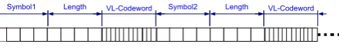
Figure5illustrates the bit-string template that we use to store

the LLH coding information (coding-info-string) which consists of symbol, length of the word for the symbol and the

code-word of the symbol, for the succession of different symbols in

the given hexadecimal layer-stamp.

In fact, a LLH-Hex layer-stamp can be decoded using the aforementioned coding-info-string, bearing in mind that accord-ing to our defined codaccord-ing-info-straccord-ing, the constant length to store

each different symbol is 4 bits, and the maximum length of each

variable-length code-word is 16 bits. After decoding a LLH-Hex layer-stamp, the resulting hexadecimal layer-stamp can be trans-lated to the attribute-values for each individual attribute in the

layer by using the information encapsulated withinatrstr and

atrpos.

In remaining of this section, we show how our resource

de-scription model is able to efficiently describe hardware capability

information of the individual peers in a system, while it provides

an efficient underlying scheme for information transmission and

communication between peers during resource discovery. In our example, we assume that we can describe the relevant hardware

capabilities, using 4 different attributes per layer. For this

pur-pose, we select and define the general system attributes using

Table1. This table also provides the values of the described

attributes for a sample single resource, as described in Listing7.

As it is shown in Table1,atrstrfor thelayer1is 0123, which

Figure 4: A) Aggregation Procedure, B) Attribute Extraction Procedure

Figure 5: Binary String Template for LLH-Hex Encoding

the values of two parameters: attribute-positioning (FFF7) and attribute-string (0123). Thus, in order to extract the values of

different attributes from the given layer-stamp, the binary stamp,

according to atrpos, must be divided to four individual parts

with the size of 16, 16, 16 and 8 bits (according to the attribute

definitions in Table1) which are corespondent to the attribute 0,

1, 2 and 3, respectively.

Table 2: Information Encoding

Layer1 Layer2 Layer3

Hex-smp 07D00800009604 0008012 20000500520064

Bin-smplength 56 bits 28 bits 56 bits

LLH-smplength 30 bits 12 bits 26 bits

LLH-smpreduction 46% 57% 53%

RLH-smplength 26 bits 12 bits 22 bits

RLH-smpreduction 53% 57% 60%

Table2provides a comparison between both LLH (our

ap-proach) and RLH (i.e., a combination of Huffman and

Run-Length algorithms) coding algorithms in terms of reduction of bits in encryption. For this comparison, we use the definition of attributes and their corresponding values (for a sample re-source) and also the values ofatrstrs andatrposs for each layer,

presented in Table1. The attributes defined are categorized in

3 layers. Hexadecimal-Stamp (Hex-smp) specifies the

result-ing layer-stamp in hexadecimal for each layer. Bin-smplength

shows the length of Binary-Stamp (number of bits) for each

layer. LLH-smplength and RLH-smplength are also the lengths

of each encoded layer-stamp using LLH and RLH encoding

accordingly. Similarly, LLH-smpreductionand RLH-smpreduction

demonstrate the rate of reduction for encoded layer-stamps for both methods. The rate of reduction is the ratio of bits-reduction (number of bits for input string minus number of bits for output string) to number of bits for input string. As we can see in Table 2, RLH provides better rate of reduction in the range of [53%, 60%] while the rate of reduction for LLH is [46%, 53%]. How-ever, the rate of reduction is not the only important performance criteria in deciding to use a coding approach, rather, there are other important aspects. Among them the cost of encoding (in terms of memory) is very important. In fact, an encoding process generally creates two type of information in output, including the encoded information and the information which is required for decoding process (e.g., coding-info-string which stores the list of symbols and their corresponding codes). For an encoding process, the cost of encoding specifies the amount of memory which is required to store encoding information (for the purpose of later decoding).

Table 3: Cost of Encoding (Required Space): NOS=Number of Fixed-Length Symbols, BPS=Required Bits per Symbol, BFL=Required Bits for the Fixed-Length, MCL=Maximum Permitted Codeword-Length, MBC=Maximum Re-quired Bits for the Codewords, LID=Length of Sample Input Data by Bits, TCB=Total Cost or Maximum Cost by Bits

NOS BPS BFL MCL MBC LID TCB

LLH-Hex n=16 4 4 l=16 n∗l=256 any-length 384 RLH-Hex n∗n=256 8 4 l=16 n∗l₌4096 any-length 7168

In Table3, we compare RLH to our LLH encoding method

in terms of encoding cost. As we can see in the table, LLH creates the maximum cost of 384 bits for each layer encoding while its rate of reduction is more than 30%. It means that using this scheme, we would be able to encode unlimited number of

attribute-values with the maximum memory cost of 384 bits

which is very low-cost. Table3also shows that despite our LLH

algorithm, the maximum memory cost for RLH is too high (7168 bits per each layer encoding). In overall, RLH provides better

rate of reduction (compared to LLH), but it significantly suffers

from its large encryption cost.

4. HARD Mechanisms

JCS environments are hierarchical and highly-heterogeneous in nature. Accordingly, the HARD architecture deploys various layer-based hybrid adaptive mechanisms (i.e.,

inter-layers and intra-layers methods) in order to efficiently

di-rect discovery requests to the proper resources across and within layers. This means that, according to properties and character-istics of each layer in the hierarchy, HARD proposes a set of specific adapted methods which have been designed to obtain

the maximum discovery efficiency on the target layer while an

integrated and coherent approach is used to traverse layers in hierarchy.

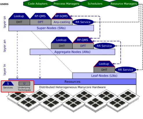
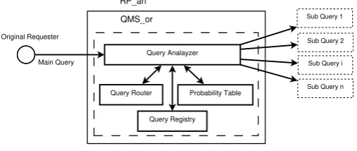
4.1. Overall System Architecture

Figure6depicts the overall architecture of HARD3,

highlight-ing users, main services, underlyhighlight-ing techniques and organization

of computing resources in different layers.

Figure 6: HARD3 Overall System Architecture

We build our system architecture based on a self organized virtual hybrid overlay. In order to create the virtual overlay, at

first, the resources in the system are organized withinvnodes

according to their homogeneity and proximity parameters (i.e.,

their similarities and locations). In the next stepvnodes start

to negotiate with each other in a multi-round distributed fash-ion to seek agreement on the contributfash-ion (i.e., module-role orvnodetype) of each party in the overlay hierarchy. As

ne-gotiations evolve, eachvnodeshapes its own system-view by

improving and consolidating its own knowledge on the entire

system. The resulting overlay contains three different types of

super-nodes (SNs) which take position in layerln, layeran and

layersn of the hierarchy respectively. Depending on thevnode

type (i.e., module-role), each virtual-node provides different

HARD3 services (e.g., QMS and SQMS).vnodes in the upper

layers are able to provide discovery services specific to their own

layer and all the services in the lower layers. vnodes respond

to the discovery demands based on their module-roles as well as the immediate requirements of the triggered communication

events. For example, avnodein layersn(i.e., a super-node)

pro-vides SQMS service. However, depending on the properties of the received communication events, it may also provide QMS or RR services or participate in the overall discovery procedure by playing a role of a leaf-node.

As it is represented in Figure 6, the leaf-nodes in layerln

are organized in distributed hash tables (DHTs) based on the multidimensional fingerprint (layer-stamp) of each participat-ing vnode. In fact, the leaf-nodes participate in a core-level specification-based DHT ring where the sibling nodes (i.e., the vnodes with similar resources) are linearly organized in linked lists with single entries on the DHT ring. Our proposed DHT ring is a variation of Chord [29] with capability to manage

sibling nodes. Similarly, aggregate-nodes (in layeran) and

super-nodes (in layersn) regardless of their module-role, participate in

DHT. For each group of LNs which elect a single AN/SN as

their common resource provider (QMS or SQMS), the DHT is

composed of all thevnodes in the group (containing LN

mem-bers and either a single AN or a single SN). In other words, allvnodes, regardless of their module-role, are able to perform

Lookupqueries over DHTs (refer to Section5.1for a detailed description of the proposed algorithm for DHT lookup).

The reason to use DHT in the core-level (layerln) of our

ar-chitecture is due to the following aspects: (a) DHT is scal-able: this is specially important when considering the potentially large number of cores that can reside on a single die (in future systems). (b) DHT is fast, reliable, fault tolerant and deter-ministic: resource discovery in the core-level is much more sensitive to speed than querying in the network-level, due to the tightly coupled design of core processors. In

many-core level, resource discovery might be ineffective if it fails to

provide required information in an adequate amount of time (e.g., discovery latency might have a direct impact on the cost of execution migration in a many-core environment). Moreover, in such highly sensitive environments, it is essential for a dis-covery method to operate reliably and provides deterministic results (undetermined results might have cost by reprocessing the query or exploring an already visited search space). (c) DHT maintenance is low cost (in terms of memory and communica-tion): a very small finger-table is required to be maintained in eachvnodein layersn. (d) DHT supports attribute-based query

description: this makes DHTs more compatible to our attribute-based resource description model. On the other hand, DHTs originally do not support semantic-based querying. To solve this issue, in our DHT variation, we enhanced the original Chord DHT to support a similarity algorithm which makes feasible similar-matching instead of exact-matching (HARD supports both modes of matching through specifying the desired matching mode in the query by the user).

QMS is a service which provides query processing

facili-ties in layeran. It uses a probability-based mechanism to guide

queries among a group of aggregate-nodes which share a single super-node as the resource provider (i.e., SQMS). During the discovery procedure, distributed probability tables (DPTs) co-operate with each other in a set of dynamic distributed learning processes, which are adapted to the progressive environmental changes. For each AN, its local probability table dynamically collects, aggregates and updates information about the status of the overall resources in the system, gathered from all transacted queries and results through the AN itself. By using this DPT technique, the network that connects ANs becomes increasingly resource-aware, as the number of traversed queries increases

across the system (refer to Section5.2for detailed description

of the proposed methods for DPTs and querying in layeran).

We use DPT as a base method in the die-level (layeran) due

to its scalability, dynamicity, efficiency and also its compact

structure. Comparing to DHT, DPT provides probabilistic results instead of deterministic results. But this not a drawback, since DPTs operate in the middle-level of HARD architecture which does not need to provide deterministic results. The reason is

that, queries are not going to be concluded in layeran. In fact, a

query processing starts from the top-level (layersn) (of course,

if there exist any query conditions for this layer) and then goes

to the middle-level (layeran) and finally it could be concluded

in the lower-level (layerln). Furthermore, we enhance our DPT

approach by introducing a SoR mechanism which can help DPT to provide deterministic results whenever feasible.

The compact design and dynamic nature of DPT provides a

facility to efficiently cope with dynamic changes in the

environ-ment (e.g., unavailability of resources due to resource failure,

resource reservation, etc). Eachvnodein layeran maintains a

small probability table. Depending on the number of predefined attributes in the system, a property table may include multi-ple records (called resource-type or resource-category records), where each record represents the aggregated probability informa-tion for all neighbors with respect to the overall query transacinforma-tion data (monitoring data), collected and analyzed, for a single at-tribute over a predefined specific range of values. In fact, each resource-type record includes probability factors for all

neigh-bors as well as a suggestion of a SoR (avnodewhich

determin-istically can provide resources, matched with the resource-type definition of the record). We also note that probability tables

only cover attributes defined for layerlnand layeran. We discuss

further details of DPT and SoR mechanisms in Section5.2.

SQMS is a specific QMS which provides additional

capabil-ities to support query forwarding in layersn. For instance, as

we can see in Figure6, super-nodes (i.e., SQMS providers) are

able to concurrently provide multiple services (such as lookup,

QMS, SQMS and RR) for the different triggered communication

events (refer to Section4.5). The query forwarding in layersn

uses the specifications of the resources in the node-level to con-duct a specification based anycasting method to direct the queries among SNs. It uses the top level layer-stamps to create anycast groups, while nodes in this layer are able to automatically adjust to the anycast group they are interested in based on their

as a base method for querying in the network-level (layersn)

due to its scalabity, efficiency and its powerful features which

make it more adequate and compatible for resource discovery in computing systems with a large number of network connected nodes (as we discussed in our previous work [30]).

Depending on the specific DOS architecture, HARD3 users could be resource management entities, schedulers, process man-agers or even code adapters. Each user would be able to perform resource discovery through invocation of a RR entity. RR in turn sends the given query to its local QMS. Due to the type of query and the user’s demand (e.g., simple single resource, multiple heterogeneous resources, complex resource graph containing the constraints for inter resource communications, etc.) QMS

splits theMain-Queryto a set of sub-queries and chooses the

appropriate layer that each sub-query must start to process. Fi-nally, the QMS that originated the sub-queries, aggregates the discovery results, and responds the RR with a set of resource

matches that optimally satisfy theMain-Query’s demand. In the

remaining of this section we elaborate more on the mechanisms proposed above.

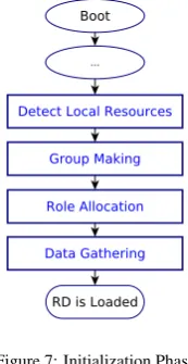
4.2. Initialization Phase

Initialization procedure is the pre-processing phase of the resource discovery process, where the initialization of the envi-ronment variables (e.g. modules configurations) is performed. In fact it is necessary in order to provide the minimum requirements for the execution of the discovery algorithm. The discovery pro-cess in the next phase is performed on the basis of these primary settings which consist of the resource grouping and clustering indexes, module roles initialization and allocation of the primary values for the underlying data structures. Some of these settings are directly calculated and stored in the local memory of each node during initialization phase while some others are

dynam-ically updated/recalculated according to different policies and

during the discovery procedure. There are also system variables which are required to be set by the system administrator such as grouping policies and grouping thresholds.

Figure 7: Initialization Phase

In summary, the initialization phase (see Figure 7) of the

resource discovery modules consists of the following steps:

1. Self-organization and self-stabilization of the multi-layers

communication overlays (zero/auto-configure overlays)

2. Distributed role-allocation (e.g., leaf-node, aggregate-node, super-node)

3. Data gathering and registration (initialization of the succes-sor, probability and neighbor tables)

The details of the algorithm for self-organization and self-configuration of the nodes in hierarchical layers (e.g., layerln,layeran andlayersn) have been presented in our

previ-ous work in [31].

4.3. Storage and Retrieval

In HARD3 initialization phase, according to a distributed self-configuration mechanism, each single HARD3 instance

(running on differentvnodes) obtains its own instance role (i.e.,

module-role), which clarifies the future operational behavior of that module instance in terms of discovery. Depending on the module role, each resource discovery instance is responsible for maintaining and updating a set of information in memory, which are the following:

A)The nodes which have the LN role maintain a successor

table, a resource state table (i.e., a vector of states for all the

resources belonged to avnode), a leaf-stamp, a pointer to the

sibling node (i.e., a vnodewith similar type of resources in

the current DHT-ring) and a QMS-ID. Successor tables in leaf-nodes are created through getting information from the system resource description provider and by leveraging some dynamic algorithms. The leaf-stamp is a key that demonstrates all the characteristics of a computing node (e.g., a processor) in the leaf-node layer and it is generated by extraction and aggregation of the predefined layer’s characteristics presented by the system resource description provider. The QMS-ID also specifies the address of a cluster representative which the current leaf-node belongs to (i.e., the address of an aggregate-node in the system which provides QMS service).

B)The nodes which have AN role (i.e., the nodes with QMS

functionality) maintain all the information related to the LN layer as well as a probability table, an aggregate-stamp and a SQMS-ID (i.e., Super-Node SQMS-ID). The probability table will be created and configured by the aggregate-node itself during initialization phase and it would be updated during the resource discovery procedure due to the dynamic behaviors of the HARD3 module instances which are running on the other aggregate-nodes in the system. Furthermore, the aggregate-stamp indicates all the characteristics of a computing node in the AN layer through extraction and aggregation of those properties from the resource description provider.

C)The nodes which have SN role (i.e., the nodes with SQMS

functionality) maintain all the information related to both of the LN and AN layers as well as the neighbors table and the node-stamp. The neighbors table provides information about the other super-nodes in vicinity and the node-stamp indicates all the predefined characteristics of a computing node in the SN layer.

procedure (resulting from a dynamic self-organization of the logical network overlays in the hierarchy). The value for module-role can be LN, AN or SN. We must also note that, each one of the module instances has the capability to act as a leaf-node by default. However they can not play the role of aggregate-node or super-aggregate-node unless their module-roles clearly are marked as such. Moreover, the role of each module instance can be changed dynamically during the resource discovery procedures, and system self-organization.

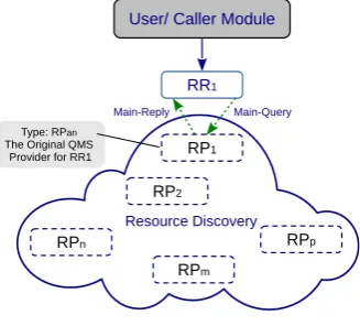
4.4. Resource Requester and Resource Information Provider RRs are the module instances that query RPs on behalf of HARD3 users (i.e., the resource discovery users or the system components such as resource manager or process manager which need to discover resources for purposes like resource allocation) for their needed resource information and the RPs are the module instances that provide information services to other RPs and RRs.

As it is shown in Figure8, RR operations can be summarized

according to the following steps:

Figure 8: Resource requester general behavior.

(1) RR reads memory to get the description of resources which are demanded by a user (reading and analyzing the user’s query description). In accordance with our hierarchical resource description, the description of the required resources can be ac-curately reflected in a flexible query description. A general query might be described as a single group of heterogeneous resources, which contain several homogeneous group of resources. The description of each homogeneous group represents the group characteristics such as number of desired resources, static and dynamic desired properties of resources in each standard layer and the required inter-resources and inter-groups communication properties.

(2) Using the query description set by the user, RR creates a

Main-Querymessage and sends it to its local QMS. The local QMS is the default self-configured RP for RR. Each local QMS, on behalf of its RR clients, manages all the relevant discovery

steps for aMain-Queryin the distributed system.

(3) Later, RR receives a main-reply message corresponding to its discovery request. This consists of information on the discovered resources which are pre-reserved for the user (i.e., application segments belonging to the user). RR is able to either release them or reserve these resources for a longer time period. The discovery temporary reservation for each resource

will automatically end after a certain time period if the related RR makes no decision on the reservation policy. Moreover, a RR will release the reserved resources when those resources are not needed any more by the user (i.e., application execution is terminated).

Unlike the irrelevancy of RR behavior to the module’s role, the RP algorithms and mechanisms are mostly dependent on the module’s role. For this reason, we elaborate on the details

of these algorithms in Section5, explaining the behavior of the

HARD3 modules from RPs viewpoint.

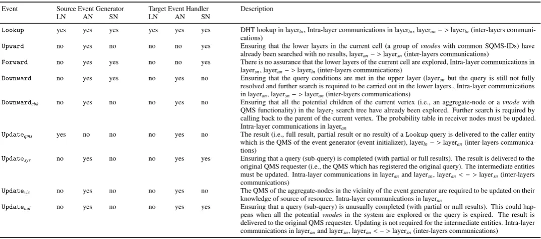
4.5. Communication Events

After the initialization phase has been completed, system ac-tions are concentrated along the line of maintaining resource information, handling queries and managing unpredictable changes in the system configuration. In order to handle queries and route discovery requests to the proper resources within and across layers, we have defined several types of events (see Figure

9and Table4) where each event specifies the type of

commu-nication and also the necessary actions that are required to be done by a receiver node. The receiver node basically acts as an event handler responsible for handling the triggered event. These events are the following:

Figure 9: Communication events within layer and across layers. Lookupevent: DHTs have been used to store the highest details of the resource information in the lowest layer of the resource description hierarchy, therefore all the peers in a

mini-cell (i.e., a group ofvnodes with common QMS-ID and

SQMS-ID) participate in a ring-based DHT. It is not necessary to have a single or flat DHT, rather in each mini-cell, for each dimension,

a flat/hierarchical ring can be used. RPs triggerLookupevents

in order to search the entire leaf-nodes in the local mini-cells for the desired resources.