A comparative study of two population models for the assessment of basis risk in longevity hedges

City, University of London Institutional Repository

Citation

:

This is the accepted version of the paper.

This version of the publication may differ from the final published

version.

Permanent repository link:

Link to published version

:

Copyright and reuse:

City Research Online aims to make research

outputs of City, University of London available to a wider audience.

Copyright and Moral Rights remain with the author(s) and/or copyright

holders. URLs from City Research Online may be freely distributed and

linked to.

A comparative study of two-population

models for the assessment of basis risk in

longevity hedges

Andr ´es M. Villegas1_{, Steven Haberman}2_{, Vladimir K. Kaishev}2_{, and Pietro}

Millossovich2,3

1_{ARC Centre of Excellence in Population Ageing Research (CEPAR), UNSW Business}

School, University of New South Wales, Sydney, Australia

2_{Cass Business School, Faculty of Actuarial Science and Insurance, City, University of}

London, United Kingdom

3_{Department of Economics, Business, Mathematics and Statistics ‘B. de Finetti’,}

University of Trieste, Italy.

ABSTRACT

Longevity swaps have been one of the major success stories of pension scheme de-risking in recent years. However, with some few exceptions, all of the transactions to date have been bespoke longevity swaps based upon the mortality experience of a portfolio of named lives. In order for this market to start to meet its true potential, solutions will ultimately be needed that provide protection for all types of members, are cost effective for large and smaller schemes, are tradable, and enable access to the wider capital markets. Index-based solutions have the potential to meet this need; however concerns remain with these solutions. In particular, the basis risk emerging from the potential mismatch between the underlying forces of mortality for the index reference portfolio and the pension fund/annuity book being hedged is the principal issue that has, to date, prevented many schemes progressing their consideration of index-based solutions. Two-population stochastic mortality models offer an alternative to overcome this obstacle as they allow market participants to compare and project the mortality experience for the reference and target populations and thus assess the amount of demographic basis risk involved in an index-based longevity hedge. In this paper, we systematically assess the suitability of several multi-population stochastic mortality models for assessing basis risks and provide guidelines on how to use these models in practical situations paying particular attention to the data requirements for the appropriate calibration and forecasting of such models.

1. INTRODUCTION

Recent years have seen a huge growth in longevity risk transfer, both in the insurer to reinsurer market, and from pension schemes to the insurance market. For example in 2014

£36.6bn of longevity risk was transferred from pension schemes to insurers and reinsurers via buy-ins, buy-outs and longevity swaps. Of this, £25.4bn related to longevity only transactions (longevity swaps), more than double the volume written in the preceding 3 years (Hymans Robertson LLP, 2015). An effective, growing market with sufficient capacity to meet demand would be to the benefit of all participants, whether to enable business to be done, or to manage risk.

solutions – where the payouts are linked to a longevity index or metric based on an external reference population – are possible. They have the potential to provide important benefits: lower costs, faster execution, potential for liquidity, and greater transparency.

In its simplest form an index based longevity swap involves a payment to the pension scheme or insurer that is based on the longevity experience of a reference index. An index-based swap provides a means to obtain (partial) protection from longevity risk both for pensioners but also deferred pensioners who are generally not covered by the “bespoke” transactions. In the case of life insurers they offer a potentially flexible way to manage exposure to longevity risk, or to facilitate a more capitally optimal balance between longevity and mortality risk. However, index-based swaps do not provide a perfect risk reduction due to the presence of basis risk, which arises from the differences in the mortality experiences of the reference population of the index and of the target population being hedged. As a result, the index based payments will not exactly match the actual annuity payments being made by the insurer or pension scheme.

There are three primary sources of basis risk driving the mismatch between the insurer or pension scheme liabilities and the longevity index hedge (LLMA, 2012):

• Structuring risk due to the payoff of the hedging instruments being different to that of the portfolio: for example the hedging instrument making annual payments whereas the portfolio pays annuities or pensions monthly, the hedge may be of shorter duration than the liabilities or it may contain some option-like features such as caps/floors or other non-linear payoff patterns.

• Sampling riskarising from the random outcomes in the mortality of the individual lives within the portfolio and the index population meaning the actual mortality experienced by the two populations will not be the same, other than by chance. The impact of sampling risk may be aggravated by concentration risk affecting the portfolio.

• Demographic risk owing to demographic and socio-economic differences in the composition of the actual portfolio being hedged and the index population referenced in the hedge, leading to different underlying mortality rates at the current moment – and in the future.

Well-established approaches for modelling the first two of these sources of basis risk exist. Structuring risk can be assessed by simulating the cashflows under the portfolio and the payoffs under the instrument, whilst sampling risk can be modelled by simulating the outcomes for the respective populations.

two populations. Li and Hardy (2011) investigate the use of a number of multipopulation extensions of the Lee-Carter model (Lee and Carter, 1992) for the assessment of basis risk and use the Augmented Common Factor model of Li and Lee (2005) to quantify the hedge effectiveness of an index-based q-forward longevity hedge. Li et al. (2015) propose a systematic approach for the construction of two-population mortality models that can be used for the quantification of the population basis risk in a standardised longevity hedge. In addition, recent years have seen a boom in the actuarial and demographic literature looking at the modelling of mortality in two (or more) related populations (e.g. Li and Lee (2005); Jarner and Kryger (2011); Plat (2009b); Cairns et al. (2011a); Dowd et al. (2011)). These two-population models, although not always proposed with the specific aim of assessing longevity basis risk, have the potential for allowing market participants to compare and project the mortality experience for the reference and target populations and thus assess the amount of demographic basis risk involved in an index-based longevity hedge. However, often the portfolio experience data will be sparse, posing a challenge for the accurate calibration and projection of the two-population model.

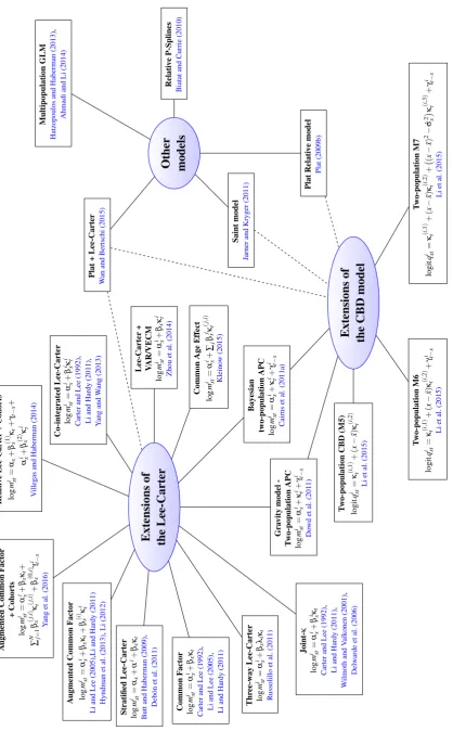
Our purpose in this paper is threefold. First, we provide a systematic and structured overview of existing multipopulation mortality modelling methodologies (c.f. Figure 1) scattered within the actuarial, demographic and statistical literature.

Our second goal is to summarize existing and formulate new criteria that a two-population mortality model should satisfy in order to be suitable for assessing basis risk.

Finally, our third goal is to systematically evaluate, contrast and select the model(s) that satisfy these criteria. We have done that by using prototype pension schemes with different size, history length and socio-economic composition. To the best of our knowledge, such a comprehensive analysis covering different characteristics of pension schemes and many alternative models has not been performed before. Our main finding is that two-populations mortality models are efficiently applied only if the scheme size exceeds 20,000-25,000 lives and its history length is at least 8-10 years. Given these conditions are satisfied, we found that the most appropriate models to be used for assessing basis risk are M7-M5 and CAE+Cohorts (see Table 3).

We believe that providing such an overview and comparison is an important contri-bution that will help researchers and industry practitioners interested in longevity risk modelling. Furthermore, we have shaped the framework under which basis risk assess-ment methodologies can reliably be used. Therefore, we have offered market participants involved in longevity transactions an invaluable analytical tool.

discuss the data requirements for the appropriate calibration and forecasting of such a model. Having identified some reasonable models for basis risk assessment, we examine in Section 7 the performance of these models in some simple illustrative hedge-effectiveness evaluation exercises, paying particular attention to the impact that different volumes of data may have on the assessment of basis risk. Finally, we conclude in Section 8 with a discussion of our main findings and future areas of research.

2. NOTATION

We denote byRthe reference population backing the hedging instrument and by Bthe book population whose longevity risk is to be hedged. We assume that for the reference population the number of deaths at agex last birthday in calendar yeart,DR_xt, and the matching initial exposed to risk,E_xtR, are available. The corresponding 1-year death rate for an individual in the reference population agedxlast birthday and in calendar yeart, denotedqR_xt, can be estimated as ˆqR_xt =DR_xtE_xtR. Similarly, the corresponding quantities for the book population are denotedDB_xt,E_xtB and ˆqB_xt = DB_xtE_xtB. We assume that these data are available for a given set of ages and given numbers of years that can differ between the reference and the book populations. More precisely, we assume thatDR_xt,E_xtR are available for consecutive agesx=x₁, . . . ,x_l and consecutive calendar yearst =t₁, . . . ,t_nR, while in the book they are available for agesx=x1, . . . ,xm and calendar yearst =u1, . . . ,unB.

Typically, data for the reference population will be available over a longer horizon than in the book, that isn_R≥n_B. Also, the set of calendar years of data in the book may be a subset of the corresponding calendar years in the reference population i.e. we may find that

u_nB 6=t_nR. Further, the ages available within the book may be a subset of those available in the reference population.

3. OVERVIEW OF AVAILABLE TWO-POPULATION MORTALITY

MODELS

In order to be able to assess basis risk, we need a model that is able to capture the mortality trends in the reference population backing the hedging instrument and in the book population whose risk is to be hedged. That is to find a suitable two-population model forqR_xt andqB_xt which produces consistent stochastic forecasts of future mortality.

Extensions of the Lee-Carter J oint-κ log m i xt = α

i x+

β

i xκ

t Carter and Lee (1992) , Li and Hardy (2011) , W ilmoth and V alk onen (2001) , Del w arde et al. (2006) Thr ee-way Lee-Carter log m i xt = α

i x+ βx λi κt Russolillo et al. (2011) Common F actor log m i xt = α

i x+ βx κt Carter and Lee (1992) , Li and Lee (2005) , Li and Hardy (2011) Stratified Lee-Carter log m i xt = αx + α i+ βx κt Butt and Haberman (2009) , Deb ´on et al. (2011) A ugmented Common F actor log m i xt = α

i x+ βx κt + β ( i ) x κ i t Li and Lee (2005) , Li and Hardy (2011) Hyndman et al. (2013) , Li (2012) A ugmented Common F actor + Cohorts log m i xt = α

i x+ βx κt

+

∑

N j=

1 β ( j , i ) x κ ( j , i ) t + β ( 0 , i ) x γ

i t−

x Y ang et al. (2016) Relati v e Lee-Carter + Cohorts log m i xt = αx + β ( 1 ) x κt +

γt−

x

+

α

i x+

β ( 2 ) x κ i t V ille g as and Haberman (2014) Co-integrated Lee-Carter log m i xt = α

i x+

β

i xκ i t Carter and Lee (1992) , Li and Hardy (2011) , Y ang and W ang (2013) Lee-Carter + V AR/VECM log m i xt = α

i x+ βx κ i t Zhou et al. (2014) Common Age Effect log m i xt = α

i x+

∑

j

β

j xκ

( j , i ) t Kleino w (2015) Bay esian tw o-population APC log m i xt = α

i x+

κ

i t+

γ

i t−

x Cairns et al. (2011a) Gra vity model -T w o-population APC log m i xt = α

i x+

κ

i t+

γ

i t−x

Do wd et al. (2011) Extensions of the CBD model T w o-population M7 logit q i xt = κ ( i , 1 ) t + ( x − ¯ x ) κ ( i , 2 ) t + ( x − ¯ x ) 2− ˆ_σ 2 x κ ( i , 3 ) t + γ

i t−x

Li et al. (2015) T w o-population M6 logit q i xt = κ ( i , 1 ) t + ( x − ¯ x ) κ ( i , 2 ) t + γ

i t−

The first ideas for modelling multiple populations go back to the seminal work of Carter and Lee (1992), who suggested three possible ways of extending their single population model (Lee and Carter, 1992) in order to forecast differentials in US mortality between men and women. The first and simplest approach suggested by Carter and Lee (1992) is to use independent Lee-Carter models for each population, and, if desired, to study in a later stage the dependence between the population-specific period effects. A second approach, the Joint-κ model, assumes that a single period componentκt drives the mortality change for all the populations but assumes that the age-specific mortality pattern and the age-specific responses to changes in the level of mortality are population-specific. The third approach estimates the populations jointly using cointegration techniques.

Formally, the Joint-κ model assumes that the central death rate at timet for agexin

populationi,mi_xt, is given by

logmi_xt =α_xi+β_xiκt. (1) Several other models proposed in the literature can be thought of as restricted versions of the Joint-κ model in Equation (1). These include: the Three-way Lee-Carter model

of Russolillo et al. (2011) which assumes that β_xi=βxλi; the Common Factor model introduced by Li and Lee (2005) where β_xi =βx; and the stratified Lee-Carter model proposed in Butt and Haberman (2009) where it is assumed thatα_xi=αx+αiandβxi=βx. The structure of the Joint-κmodel and of its restricted versions imply that mortality

improvements are perfectly correlated across populations. Moreover, the Common Factor and Stratified Lee-Carter models imply the same mortality improvements for all population at all times. However, since this is an unrealistic assumption for most datasets, Li and Lee (2005) have added a population specific factor to the Common Factor model, in the so-called Augmented Common Factor model:

logmi_xt =α_xi+βxκt+βxiκti. (2) In Equation (2) the term β_xiκ_ti captures the deviations of the rate of mortality change

of population i from the long-term trend in mortality change implied by the common factor,βxκt. In order to avoid divergence in the projected mortality, Li and Lee (2005) assume that theκ_tifactors can be modelled using stationary processes such as a first order

autoregressive process, AR(1). Under this modelling assumption the mortality rates of the different populations may wander apart in the short and medium terms, but tend to converge in the long-run. The Augmented Common Factor has spawned several variants and extensions. Hyndman et al. (2013) have introduced the product-ratio method which extends the Augmented Common Factor model by adopting a functional data approach and allowing more than one period index for the modelling of both the common factor and of the population-specific factors. Li (2012), who also considers multiple period indexes, uses a Poisson setting to estimate the parameters of the Augmented Common Factor model instead of the singular value decomposition approach originally employed by Li and Lee (2005). Recently, Yang et al. (2016) have extended the Poisson Augmented Common Factor to allow for possible cohort effects. Villegas and Haberman (2014) have considered a similar cohort variant of the Augmented Common Factor for the purpose of studying socio-economic differences in mortality.

As discussed in Li and Hardy (2011), to implement a two-population version of the co-integrated Lee-Carter model suggested by Carter and Lee (1992), one must first fit two independent single population Lee-Carter models to each of the populations,

and then model jointly the period effects of the populations,κ_t1andκ_t2, with a co-integrated

bivariate process under the assumption of the existence of a common stochastic long-term trend linking the mortality of the two populations. In the same vein, Yang and Wang (2013) fit independent single population Lee-Carter models to multiple populations and then model simultaneously the period effects of the different populations using a Vector Error Correction Model. In order to impose further consistency in the forecast of the two-populations, Zhou et al. (2014) assume in (3) that both populations share the same age-sensitivity term, i.e.β_xi=βx. For modelling the period indexesκt1andκt2, Zhou et al. (2014) consider three methods: a random walk with drift forκ_t1plus an AR(1) forκ_t2−κ_t1

(abbreviated RWAR by the authors), a vector autoregressive model (VAR); and a Vector Error Correction Model (VECM). Similarly to Zhou et al. (2014), Kleinow (2015) has proposed a multiple population Common-Age-Effect model in which the age-sensitivity terms (age-effects) are common to all the populations.

Another alternative for modelling multi-population mortality is to extend the widely used single-population Cairns-Blake-Dowd (CBD) model of mortality (Cairns et al., 2006). This approach has recently been considered by Li et al. (2015) who introduce population versions of the CBD model and its variants. For instance, in a full two-population version of the M7 model (the CBD model with cohort and quadratic effects proposed in Cairns et al. (2009)), the one-year death rate for a person agedxat timet in populationi,qi_xt, is given by:

logitqi_xt =κ_t(i,1)+ (x−x¯)κ_t(i,2)+ (x−x¯)2−σˆ_x2κ_t(i,3)+γ_ti_−x, i=1,2, (4)

where ¯xis the average age in the data and ˆσ_x2 is the average value of(x−x¯)2. Li et al.

(2015) also set out a systematic top-down procedure to evaluate if some of the stochastic factors in the two-population model can be shared by the two populations (e.g. by assuming in (4) thatκ_t(1,j)=κ_t(2,j)for some j∈ {1,2,3}or thatγ_t1_−x=γ_t2_−x). For model forecasting

Li et al. (2015) consider the same three approaches used by Zhou et al. (2014).

In two closely linked studies looking at the mortality dynamics of a pair of related populations, Cairns et al. (2011a) and Dowd et al. (2011) have proposed the use of a two-population version of the Age-Period-Cohort (APC) model:

logmi_xt =α_xi+κ_ti+γ_ti_−x, i=1,2. (5)

In both studies, the spreads between the state variables underlying the mortality models of each population are modelled as mean-reverting processes (e.g. an AR(1)) allowing different short-run trends in the mortality rates, but parallel long-run improvements. Cairns et al. (2011a) employ a Bayesian framework permitting a single stage estimation of the unobservable state variables and the parameters of the stochastic process driving them. Dowd et al. (2011) use a planetary analogy in which the mortality of the two populations are attracted to each other by a dynamic gravitational force dependent on the relative size of the populations.

with the mortality experience of a much larger reference population. They assume that the reference population follows a deterministic long-run trend which is shared with the small population, and then model short term deviations of the small population from that trend using a multivariate stationary time series. Similarly, Wan and Bertschi (2015) model the larger population using the multi-factor single population model proposed by Plat (2009a) and then model the spread between the larger population and the smaller population with a three factor Lee-Carter model. In a related study, Plat (2009b) introduces a model for forecasting portfolio specific mortality alongside the relevant national population. In this model, portfolio specific mortality forecasts are obtained by combining national mortality projections derived from a standard single-population CBD model, with forecasts of the ratio between portfolio mortality rates and national population mortality rates. It is worth noting that Jarner and Kryger (2011), Wan and Bertschi (2015) and Plat (2009b) adopt the same approach for modelling the factors driving the dynamics of the mortality ratios and use a vector autoregressive model of order 1, VAR(1), so to avoid any long-term divergence of the mortality in the two populations.

Some authors have considered the use in a multipopulation setting of other well-known single population modelling approaches. For instance, Biatat and Currie (2010) extend to two populations the P-spline methodology (Currie et al., 2004) that has been successfully applied in the single population case, while Hatzopoulos and Haberman (2013) and Ahmadi and Li (2014) use the framework of generalised linear models (GLM) to obtain coherent morality forecasts for multiple populations.

4. MODELLING THE REFERENCE AND THE BOOK

POPULA-TION: A GENERAL FORMULATION

Along the same lines of the general formulation of single population models considered in Hunt and Blake (2015b) and Villegas et al. (2015), we have identified a general framework under which most two population models that have been introduced in the literature can be accommodated. However, in order to facilitate the comparison between models, the way such models are proposed here may slightly differ from their original formulation.

4.1. Reference population

Following Villegas et al. (2015), a general model for the reference population can be written as1

DR_xt ∼Bin(E_xtR,qR_xt),

logitqR_xt =α_xR+

N

∑

j=1

βx(j,R)κ

(j,R)

t +γtR−x. (6) In Equation (6) the term α_xR determines the reference mortality level for age group x;

the integerN indicates the number of age-period terms describing the mortality trend for the reference population; each time indexκ_t(j,R) contributes to specifying the reference

mortality trend with each coefficientβx(j,R) dictating how mortality in the corresponding age groupxreacts to a change in the time indexκ_t(j,R); and the termγ_tR_−xaccounts for the

cohort effect in the reference population.

4.2. Book population

Given the reference population model, the mortality of the book population is then specified through

DB_xt ∼Bin(E_xtB,qB_xt),

logitqB_xt−logitqR_xt =α_xB+

M

∑

j=1

βx(j,B)κ_t(j,B)+γ_tB_−x. (7)

Note that we are modelling the difference in the (logit of) mortality in the book and the reference populations. Therefore, in Equation (7) the termα_xB determines the mortality

level differences of the book population compared to the reference population for age groupxwith the mortality level in the book beingα_xR+α_xB; the integerM(generally less than or equal toN) indicates the number of age-period terms describing the mortality trend differences between the book population and the reference population; each time index

κ_t(j,B) contributes in shaping the difference in mortality trends with each coefficientβx(j,B) dictating how mortality differences for age groupxreact to a change in the time index

κ_t(j,B); and the termγ_tB_−xaccounts for the differences in cohort effect in the two populations,

with the cohort effect in the book beingγ_tR_−x+γ_tB_−x.

Depending on how the model is specified, identification constraints may have to be added to (6) and (7) to ensure uniqueness of the parameter estimates. The estimation of the parameters of the model can be performed using maximum likelihood in two stages whereby the reference population part of the model is estimated in a first stage and then, conditional on the reference population parameters, the book population part of the model is estimated in a second stage.2

1_{Here, we have chosen to work with one-year death probabilities,q}

xt. Therefore, it is most natural to use

the logit function and model deaths using a Binomial distribution. However, if interested in central death rates,mxt, or the force of mortality,µxt, then the general modelling framework can be easily reformulated

using a log link function and a Poisson Distribution. In addition, based on our experience, no material differences are to be expected in the analysis if central death rates,mxt, or the force of mortality,µxt, were

considered instead.

2_{An alternative approach would be to estimate simultaneously the parameters in the reference and book}

4.3. Time series dynamics

The modelling is completed by specifying the dynamics of the period indices and the cohort terms which are needed for forecasting and simulating future mortality. Although alternatives have been explored by some authors (see e.g. Zhou et al. (2014)) for the choice of the time series used in the dynamics, we stick to those commonly used in the literature.

Starting with the reference population, we assume that the period index is modelled as a multivariate random walk with drift (MRWD)

κR_t =d+κR_t−1+ξ_tR, ξ_tR∼N(0,ΣR), κR_t =

κ_t(1,R), . . . ,κ_t(N,R)

0

,

and that the cohort index is modelled as an integrated auto-regressive process ARIMA(1, 1, 0)

∆γ_cR=φ0+φ1∆γcR−1+εcR, εcR∼N(0,σR2),

where d is an N-dimensional vector of drift parameters; ∆γ_cR denotes γ_cR−γ_cR₋₁ with

c=t−x;φ0andφ1are the drift and autoregressive parameters associated with the cohort

effectγ_cR; andΣRis theN×N variance-covariance matrix of the multivariate white noise

ξ_tR.

As for the book population, we follow the assumption commonly made in the literature (Li and Lee, 2005; Plat, 2009b; Cairns et al., 2011a; Jarner and Kryger, 2011; Li and Hardy, 2011; Hyndman et al., 2013; Wan and Bertschi, 2015). More precisely we assume that in the long-run the two populations experience similar mortality improvements and therefore model the spread in the time indexes and cohort effects as stationary processes:

κ_tB=Φ0+Φ1κB_t−1+ξ_tB, ξB_t ∼N(0,ΣB), κ_tB=

κ_t(1,B), . . . ,κ_t(M,B)

0

, (8)

γ_cB=ψ0+ψ1γcB−1+εcB, εcB∼N(0,σB2),

whereΦ0andΦ1are anM-dimensional vector and anM×Mmatrix of model parameters;

ΣB is theM×M variance-covariance matrix of the multivariate white noiseξB_t; andψ0

andψ1are parameters associated to the cohort spreadγcB. Thus:

• The time indices κ_tB are modelled as a vector auto-regressive process of order 1

(VAR(1)), for which we assume that the eigenvalues of the matrixΦ1are smaller

than 1 in absolute value.

• The cohort difference γ_cB follows an AR(1) process for which we assume that

ψ1<|1|.

• We are assuming independence of the time series determining the reference pop-ulation and those determining the difference between the reference and the book populations.3

Overall, the time series dynamics approach considered here corresponds to the RWAR approach discussed in Zhou et al. (2014) and Li et al. (2015).

book population has a small size relative to the reference population. Furthermore, for some models such as the two-population APC, CBD, M5 and M7 where the log-likelihood is separable, a two-stage estimation approach results in exactly the same parameter estimates as a joint estimation approach.

3_{Considering correlations between}

ξR_t andξ_tBor betweenε_cRandε_cBis in principle possible, as has been

5. MODEL SELECTION CRITERIA

With over 20 two-population models currently proposed in the literature (see Figure 1), our main goal is to identify which model(s) are most likely to provide a satisfactory solution for assessing basis risk. In order to support this analysis, it is useful to test each model against certain criteria that a good and practical two-population model for basis risk assessment should satisfy. Building on the literature comparing single population models (e.g. Continuous Mortality Investigation (2007); Cairns et al. (2008, 2009, 2011b); Haberman and Renshaw (2011)), we consider the following criteria. The model should:

1. Produce anon-perfect correlationbetween mortality rates in the two populations. 2. Produce a non-perfect correlation between year-on-year changes in mortality at

different ages.

3. Permit thegeneration of sample pathsand the calculation of prediction intervals. 4. Have a structure that allows the incorporation ofparameter uncertaintyin

simula-tions.

5. Permit the consideration of acohort effectif necessary.

6. Becompatible with the datathat are likely to be available when doing basis risk exercises.

7. Be straightforward to implement using standard statistical methods likely to be available to practitioners.

8. Betransparentenough so that the model assumptions, limitations and outputs are understood by the users and can be easily explained to non-experts.

9. Show a reasonablegoodness-of-fitto historical data in both the reference population and the book population for a wide range of book populations.

10. Show a reasonablegoodness-of-fitfor metrics involving the two populations such as differences or ratios in mortality rates or life expectancies for a wide range of book populations.

11. Be relativelyparsimonious.

12. Produceplausible and reasonable central projectionsof both single-population and two-population metrics.

13. Produceplausible and reasonable forecast level of uncertaintyin projections of both single-population and two-population metrics, which are in line with historical levels of variability.

14. Produce parameter estimates and model forecasts that are robust relative to the period of data and range of ages employed.

Most of the above criteria coincide with the criteria that a good single population model should satisfy; we thus refer the reader to Continuous Mortality Investigation (2007, Section 8) and Cairns et al. (2008, Section 3) for a detailed discussion of their relevance. By contrast, criteria 1, 10, 12 and 13, referring to correlations between the mortality rates in the two populations and to the performance of the models in relation to two-population metrics, are new. The latter criteria are of prime importance to the application of two-population models in the assessment of basis risk in standardised longevity hedges. On the one hand, if a model assumes a perfect correlation between mortality rates in the two populations then it will imply that the reference population provides a perfect match for the book population, trivially leading to no (or very little) demographic basis risk. On the other hand, since demographic basis risk emerges from the mismatch in the mortality of the reference and the book population, it is critical that the two-population model shows a good fit to metrics involving the two populations, and that forecast levels of uncertainty and central trajectories for these metrics are plausible and consistent with historical differences between the populations.

We note however, that a two-population model which might not be suitable for basis risk assessment, may be an appropriate model for other applications in which some of the above criteria would be superfluous. For example, consider the case of valuing the liabilities of a pension book with sparse data, where we may consider a two-population model to borrow information from a larger reference population with the objective of improving the accuracy in the projections of the pension schemes’ mortality. In this situation, having a non-perfect correlations between the mortality of the two populations would be unnecessary and the performance of the model relative to two-population metrics would be of lesser importance.

6. IDENTIFYING AN APPROPRIATE TWO-POPULATION MODEL

Given the wealth of models available and the large number of criteria, we have followed a two-stage filtering process to identify the model structures likely to be suitable for basis risk assessment. In a first stage, we focus on criteria 1 to 8 which refer to theoretical properties of a model and can be evaluated without reference to a specific dataset. Then, in a second stage, we focus on criteria 9 to 14 which can only be evaluated after a model has been fitted to data. More specifically, in the second stage of filtering we evaluate the goodness of fit, the reasonableness of the output, the forecasting performance and the robustness of those models which pass the first stage of filtering.

6.1. Stage 1 of filtering: Criteria requiring no data to assess

We first evaluate all the candidate models against those criteria that can be assessed inde-pendently of data or the actual fitting of the models. This process permits the identification of a number of models which could be rejected, either because their theoretical properties are not suitable for basis risk assessment or because they are unlikely to be accessible to the wider industry.

6.1.1. Non-perfect correlation between mortality rates in the two populations

in the mortality of the reference population.4 This will result in the model spuriously suggesting that there is no (or very little) demographic basis risk. This is the case for those Lee-Carter based models with a single common period effect for both populations, leading us to view the Stratified Lee-Carter, the Common Factor Model, the Three-way Lee-Carter, and the Joint-κ model as inadequate models for assessing demographic basis risk.

6.1.2. Non-perfect correlation between year-on-year changes in mortality at differ-ent ages

This criterion refers to the correlation betweenqR_x,t+1−qR_x,t andqR_y,t+1−qR_y,t (or between

qB_x,t+1−qB_x,t and q_yB_,t+1−q_yB_,t) for x6=y. As noted by Cairns et al. (2008), a model that assumes a perfect correlation between changes in mortality at different ages would incor-rectly suggest that holding a derivative instrument linked to a single age would provide just as good a hedge as holding several instruments linked to a range of different ages. Dis-regarding this issue can result in a misassessment of the structuring basis risk underlying a longevity hedge.

Lee-Carter type models with a single period effect and no cohort effect, such as the Cointegrated Lee-Carter and the Lee-Carter+VAR/VECM, have a trivial age correlation structure. In addition, the two-population APC model in Equation (5) implies that there is perfect correlation at all ages except at the youngest ages, where there is potentially additional randomness arising from the arrival of new cohorts with an unknown cohort effect (see Cairns et al. (2009)). In contrast, two-population extensions of the CBD model allow for imperfect correlations between annual changes in mortality at different ages due to the presence of multiple period factors.

We do not discard however any model due to its age correlation structure for two reasons. In many instances it may only be required to perform an indicative assessment of the demographic basis risk associated with an index-based hedge, without necessarily considering in detail the precise structuring of the hedge. Further, in order to assess model risk, it may be useful to consider an alternative model to the one used in structuring the hedge.

6.1.3. Generation of sample paths

Mortality sample paths are required for the assessment of the uncertainty in the cash-flows of a mortality-linked security as well as for the pricing and structuring of a longevity hedge. A distinguishing feature of the P-Spline model of Biatat and Currie (2010) and of the multipopulation GLM of Ahmadi and Li (2014) is that they assume that mortality follows a deterministic time trend, meaning that these models cannot generate sample paths. Hence, we do not consider these two models any further.

6.1.4. Parameter uncertainty

Given that in most cases the amount of data for the book populations is limited, the parameters of the models may be subject to significant estimation error. It is thus important to be able to consider the impact that parameter risk can have on forecasts levels of uncertainty and on hedge effectiveness. With the exception of the Bayesian two-population

4_{Note that the correlation between the mortality ratesq}B

xtandqRxtmay not be perfect, although it will be

close to one, even when correlation is perfect on the logit scale used by the models introduced in Section 4. Also note that having a perfect correlation between the populations does not necessarily imply that he two populations experience exactly the same mortality improvements. For instance, the Joint-κ and the

model of Cairns et al. (2011a) which naturally accounts for parameter uncertainty, none of the studies we have reviewed considers parameter uncertainty. Nevertheless, for most of the models it is possible to incorporate parameter uncertainty using bootstrapping techniques such as the ones proposed in Brouhns et al. (2005), Koissi et al. (2006) and Renshaw and Haberman (2008). We should mention however that, unlike the Bayesian framework, bootstrapping is related to the effect of sampling variation in the data. Therefore by means of bootstrapping it is not possible to assess the parameter uncertainty arising from the time series processes, but rather only that due to sampling variation.

6.1.5. Cohort effect

For some countries, including England and Wales, it is important that models allow for the now well-accepted cohort effect, separating out general improvements over time to those specific to a given birth cohort. Although not all the models include a cohort effect, they can in principle be extended to include such an effect.

6.1.6. Compatibility with available data

The data requirements of some of the models are incompatible with the likely available data. For instance, it is unlikely that the book population will provide the same length of history as the reference population, hindering the application of models which cannot easily deal with such a scenario. In particular, this requirement leads to the rejection of two further Lee-Carter based models, namely the Lee-Carter VAR/VECM and the Co-integrated Lee-Carter.

6.1.7. Ease of implementation and transparency

Ease of implementation and transparency are essential for a model to be of general use by practitioners. Accordingly, these two criteria lead to the rejection of several other models. In particular, the Multipopulation GLM of Hatzopoulos and Haberman (2013) is considered to be impractical for basis risk assessment as it is a complex model which is computationally involved to implement and may be difficult to communicate to non-experts. In addition, we disregard the Plat+Lee-Carter model of Wan and Bertschi (2015) (apart from other reasons discussed later) because it combines a parametric structure for the reference with a non-parametric structure for the book, and we believe that for the sake of interpretability of the parameters both parts of the model should be within the same class of models. Finally, although the Bayesian two-population APC model of Cairns et al. (2011a) is particularly amenable to the short history and modest exposures sizes of most book datasets, the implementation and transparency issues related to the underlying Bayesian approach have led us to rule out this model. However, some of the features of the approach of Cairns et al. (2011a) will still be investigated subsequently in this paper through a maximum-likelihood implementation of the two-population APC model.

6.2. Stage 2 of filtering: Criteria requiring data to assess

After carrying out the initial data-independent assessment, the following 10 models can be identified as candidates which are worth testing against the data dependent criteria: the Augmented Common Factor model and its cohort extension, the Relative Lee-Carter model with cohorts, the Common Age Effect Model, the two-population APC (Gravity model), the two-population M5, the two-population M6, the two-population M7, the Saint model, and the Plat relative model.

Table 1. Description of the book datasets used for model testing. Q1 represents the least deprived quintile of England and Q5 the most deprived quintile.

Percentage of exposure

Dataset Description by IMD quintile

Q1 Q2 Q3 Q4 Q5

Typical Lives

This is the typical IMD split we would expect to see in a book population weighted by lives (head-count)

23% 22% 21% 20% 14%

Typical Amounts

This uses the same split as the typical (lives) but weighted by individual pension amounts to approximate the effect of a typical portfo-lio’s liability distribution amongst the IMDs

30% 25% 20% 15% 10%

Extreme Wealthy

This reflects the split by IMD (on an amounts weighted basis) that we would expect to see in a very affluent book population

45% 30% 20% 5% 0%

Extreme Deprived

This reflects the split by IMD (on a lives weighted basis) that we would expect to see in a book skewed towards lower socio-economic groups

10% 15% 15% 25% 35%

by the models, and the evaluation of the forecasting performance and robustness of the models.

6.2.1. Data

The evaluation of the criteria in this stage requires data for model fitting. We have used as the reference population data the England and Wales male mortality experience as obtained from the Human Mortality Database (2013). For the purposes of our analysis we have focused on a subset of these data covering calendar years 1961-2010 and those older ages most relevant to longevity hedging, namely ages 60-89.

For the book population we use synthetic datasets generated based on England mortality data by quintiles of the Index of Multiple Deprivation 2007 (IMD 2007)5and the socio-economic composition observed within individual occupational pension schemes of the Club Vita dataset.6 Specifically, the synthetic datasets used throughout this paper have been generated by randomly sampling from the national IMD data to obtain a dataset of exposure size, history length, and IMD profile desired. The technical details of this data sampling process are described in Appendix A. The use of synthetic data as opposed to actual pension scheme data facilitates a more thorough assessment of the models. Concretely, synthetic datasets permit us to control some key characteristics of the book population data while changing others. For instance, it allows us to vary the history length and exposure size of the book data whilst keeping the socio-economic and age composition constant. Moreover, synthetic datasets let us rely on the longer history of the national IMD mortality data to perform backtesting exercises such us those described in Section 6.2.7.

5_{A detailed analysis of the mortality data used in this paper can be seen in Villegas and Haberman (2014)}

or in Lu et al. (2014). For further information on the Index of Multiple Deprivation see Noble et al. (2007).

6_{Club Vita is an organisation which provides longevity analytics to pension schemes. The schemes in the}

● ●●

● ●

● ●

● ●

● ●

● ●●●

● ●

● ●●●

● ●●

● ●

●

● ●

●

0.8 0.9 1.0 1.1 1.2

60 70 80 90

age

Book / England and W

ales

● Typical Lives

Typical Amounts Extreme Wealthy Extreme Deprived Mortality ratio to England and Wales by age

●● ●

●● ●●

●●●●●● ●

●● ●

● ●

● ●

●

● ●●

● ●

● ●

●

0.9 1.0 1.1

1980 1990 2000 2010

year

Book / England and W

ales

Mortality ratio to England and Wales by year

Figure 2.Ratio of the mortality in each of the four synthetic book datasets to the

mortality in England and Wales. The left graph shows this ratio by age while the one on the right presents the time evolution of this ratio.

For the assessment of the goodness-of-fit of the models, we consider four different synthetic datasets to reflect the variety of socio-economic mixes observed in real pension schemes and annuity books. In each case, the socio-economic splits are motivated by the profiles seen within the Club Vita dataset. Table 1 describes the socio-economic profiles of these datasets. In all cases we use sample books with historical exposures of 100,000 male lives per year, which we believe is reasonable proxy for the largest exposure any pension scheme or insurer is likely to have. We also assume that book data are available for the period 1981-2010 and ages 60 to 89. Finally, we use the age distribution of the English population to split by age the total exposure of each of the sample schemes.

Figure 2 depicts the ratio of the mortality in each of the four datasets to the mortality in England and Wales. We note that the ordering of the ratios in the four datasets is consistent with their socio-economic mixes: the “Extreme Wealthy” dataset has below average mortality (ratio<1), the “Extreme Deprived” dataset has above average mortality (ratio>1), and the “Typical Lives” and “Typical Amounts” datasets exhibit a mortality ratio close to 1 due to the similarity of their socio-economic mix with that of England and Wales. It is also worth noticing that none of the datasets shows any very marked increasing or decreasing time trend in the mortality ratios, albeit there is a slight upward trend in the “Extreme Deprived” dataset. This is consistent with the slower mortality improvements for

the two most deprived quintiles of England reported by Villegas and Haberman (2014).

6.2.2. Model fitting

To facilitate the fitting of the 10 models that passed our first-stage filtering, we have followed the general modelling framework described in Section 4 whereby each model can be viewed as a model for the reference population combined with a model for the book population (or perhaps more accurately, a model for the mortality ratio between reference and book). As such, the fitting and the assessment of the goodness-of-fit of a model can be carried out in two stages: fitting and assessing the goodness-of-fit of the reference model, followed by the fitting and the assessment of the goodness-of-fit of the book part of the model.7 We note that conclusions regarding the goodness-of-fit of the model to

7_{All the model fitting performed in this paper has been carried out using theRpackage StMoMo (Villegas}

Table 2. Mathematical description of the models selected for the reference population.

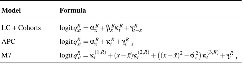
Model Formula

LC + Cohorts logitqR_xt =α_xR+β_xRκ_tR+γ_tR_−x

APC logitqR_xt =α_xR+κ_tR+γ_tR_−x

M7 logitqR_xt =κ_t(1,R)+ (x−x¯)κ_t(2,R)+ (x−x¯)2−σˆ_x2κ_t(3,R)+γ_tR_−x

the reference may lead us to slightly modifying the original formulation of certain of the two-population models before assessing the goodness-of-fit of the book part of the model. The specific modifications for each particular two-population model are described later in this section.

6.2.3. Selection of reference population

In order to identify an appropriate model for the England and Wales reference population, we have carried out an extensive evaluation of the goodness-of-fit of a number of candidate single population models. However, for the sake of brevity, we present here only the conclusion of this evaluation, but details can be followed in Haberman et al. (2014, Section 6.2.2.3).

Consistently with the existing literature which compares single population mortality models for the England and Wales population (see e.g. Cairns et al. (2009) and Haberman and Renshaw (2011)), we have found that the three models presented in Table 2 are appropriate for modelling the mortality in the reference population. In Table 2, the model labelled LC+Cohorts is one of the Renshaw and Haberman (2006) cohort extensions of the Lee-Carter model while the APC model is a special case of the LC+Cohorts where it is assumed thatβ_xR=1. Model M7 is an extension of the original CBD model and was

proposed in Cairns et al. (2009). A common characteristic of these three models is that they all include a cohort term to capture the well-known effect of year-of-birth on England and Wales mortality (Willets, 2004).

6.2.4. Goodness-of-fit for book population

In line with the models selected for the reference population, we have adapted several of the candidate two-population models before carrying out further goodness-of-fit assessments. Specifically, we have made the following adaptations:

• The Common Age Effect model, as proposed in Kleinow (2015), does not include a cohort effect. Therefore, given that there is strong evidence of a cohort effect in England and Wales, in our testing we extend this model to include such an effect. The reference population model is then a LC+Cohorts model.

• Similarly, for the Augmented Common Factor model we should consider a cohort effect, but doing so would turn the model into the Relative Lee-Carter model with cohorts. Consequently, the Augmented Common Factor model is not considered further in the analysis.

• For the Relative Plat model we assume an M7 model for the reference population as opposed to the M5 model originally assumed by Plat (2009b). In addition, while Plat (2009b) models directly the mortality ratio between the reference and the book population, qB_xtqR_xt, we model the difference in logits of mortality rates, logitqB_xt−logitqR_xt.

• For the Saint model, instead of the frailty-type model considered originally by Jarner and Kryger (2011) which we believe is too complex to be accessible to practitioners and does not permit the generation of sample paths, we use an M7 model for the reference population.

For comparison purposes, in some of our additional goodness-of-fit and reasonableness testing we will consider the Common Factor Model with added cohorts. This model, which was previously deemed inappropriate as it unrealistically implies zero basis risk, is useful for illustrating some of the undesirable characteristics in a model for basis risk assessment.

Table 3 summarises the models whose goodness-of-fit will be investigated further. The parameter constraints associated with these model structures are described in Ap-pendix B. The Common Factor model with cohorts (CF+Cohorts), the Common Age Effect model with cohorts (CAE+Cohorts), and the relative Lee-Carter model with co-horts (RelLC+Coco-horts) belong to the Lee-Carter family of models. The CF+Coco-horts only allows for level differences between the reference and the book population, whilst the CAE+Cohorts and the RelLC+Cohorts also allow for improvement differences. Never-theless, the latter two models differ in the specification of the age-modulating factorβ_xB

accompanying the book-specific time indexκ_tB: in the RelLC+Cohortsβ_xB is estimated

directly from the observed logit difference of mortality between the book and reference data while in the CAE+Cohortsβ_xBis borrowed from the reference population model, i.e.,

β_xB≡β_xR.

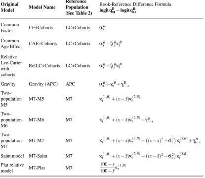
The Gravity model corresponds to a Binomial-logit version of the two-population APC introduced in Equation (5).

Models M7-M5, M7-M6, M7-M7, M7-Saint, and M7-Plat (which are the implemented versions of the two-population CBD, the two-population M6, the two-population M7, the Saint model, and the Relative Plat model, respectively) all belong to the CBD family of models. These models differ in the type of differences between the book and the reference population that are allowed for in the parametric age functions: M7-M5 and M7-M6 allow only for level and slope differences with M6 also allowing for cohort differences; M7-Saint, M7-M7 allow for level, slope and curvature differences with M7 also allowing for cohort differences; and M7-PLAT is a constrained version of M7-M5 assuming that at age 100 there is no difference between the reference and the book.

A good two-population model should show a reasonable fit to the historical mortality rates in both the reference population and the book population. In addition, the model should show a good fit to metrics involving the two populations such as differences or ratios of mortality rates. This last criterion is very relevant as demographic basis risk emerges from the mismatch in the mortality of the reference and the book population.

Table 3. Mathematical description of the two-population models considered for goodness-of-fit assessment. CF+Cohorts = Common Factor model with cohorts; CAE+Cohorts = Common Age Effect model with cohorts; RelLC+Cohorts = Relative Lee-Carter model with cohorts; M7-X = Two-population model where the reference population follows an M7 model and the book-reference difference is specified through a model of type X. See Table 2 for the corresponding reference population models.

Original

Model Model Name

Reference Population (See Table 2)

Book-Reference Difference Formula

logit qB_xt−logit qR_xt

Common

Factor CF+Cohorts LC+Cohorts α

B x

Common

Age Effect CAE+Cohorts LC+Cohorts α

B x+βxRκtB

Relative Lee-Carter with cohorts

RelLC+Cohorts LC+Cohorts αxB+βxBκtB

Gravity Gravity (APC) APC α_xB+κ_tB+γ_tB_−x

Two-population M5

M7-M5 M7 κ_t(1,B)+ (x−x¯)κ_t(2,B)

Two-population M6

M7-M6 M7 κ_t(1,B)+ (x−x¯)κ_t(2,B)+γ_tB_−x

Two-population M7

M7-M7 M7 κ_t(1,B)+ (x−x¯)κ_t(2,B)+ (x−x¯)2_−σˆ2

x

κ_t(3,B)+γ_tB_−x

Saint model M7-Saint M7 κt(1,B)+ (x−x¯)κ

(2,B)

t + (x−x¯)2−σˆx2

κt(3,B)

Plat relative

model M7-Plat M7

100−x

100−x¯κ

(1,B)

t

observed period survival probabilities in the book and the corresponding plots for ratios of period survival probabilities in the book and the reference can give useful insight into the goodness-of-fit of the models. As an illustration, Figure 3 depicts, for a selection of models, the fitted and observed 30 years period survival probabilities at age 60 for the “Extreme Wealthy” and the “Extreme Deprived” sample schemes as well as the corresponding fitted and observed ratios of period survival probabilities between both sample schemes and the England and Wales reference. Figure 3 is representative of the detailed analyses we have carried out and which have helped with our assessment of the performance of the different models under consideration.

●● ●● ● ● ●●● ● ● ● ● ●●● ● ● ● ● ● ● ● ● ● ● ●● ● ● ● ●● ● ●● ● ●● ● ● ● ● ●● ●● ● ● ● ●●● ● ●● ● ● ●● Extreme Wealthy Extreme Deprived 0.05 0.10 0.15 0.20 0.25

1980 1990 2000 2010

calendar year CF + Cohorts

RelLC + Cohorts M7−M5 M7−Plat

30p60,t

B vs. t ● ● ● ● ● ● ● ● ● ● ●●● ● ● ●● ● ● ●● ● ● ● ● ●●● ● ● ● ● ● ●● ● ● ●● ● ● ● ●● ●●●● ●● ●●●● ● ●● ●● ● Extreme Wealthy Extreme Deprived 0.8 1.0 1.2 1.4 1.6

1980 1990 2000 2010

calendar year

CF + Cohorts RelLC + Cohorts M7−M5 M7−Plat

30p60,t

B

30p60,t

R vs. t

Figure 3.Fitted vs. observed 30 year period survival probabilities at age 60 for the

“Extreme Wealthy” and the “Extreme Deprived” sample schemes. Left panel presents result for the book populations while the right panel presents results the corresponding results for ratios with respect to the England and Wales reference population. Dots in the graphs represent observed quantities.

we note:

• For the “Extreme Deprived” dataset the M7-Plat model shows a stark bias in the fitted ratios consistent with the underestimation seen in the period survival probabilities in the book population. In an attempt to improve the fit of the M7-Plat model, instead of assuming that crossing of mortality between the reference and book population occurs at the prefixed age 100, we have treated the age of crossing as an additional parameter that needs to be estimated from the data. This has however not eliminated the bias issues suggesting that the M7-Plat model might be too restrictive for some datasets. Therefore we do not consider the M7-Plat model further as a candidate for basis risk assessment.

• The CF+Cohorts and the RelLC+Cohorts models produce very smooth ratios of survival probabilities which seem to understate the observed volatility in the ratios. Whilst the poor performance of the CF+Cohorts model was expected due to the per-fect correlation between populations assumed by this model, the poor performance of RelLC+Cohorts was not.

• Further investigation of the parameters of the RelLC+Cohorts indicates that the over-smoothed fitted ratios can be linked to the presence of a book-specific non-parametric β_xB which needs to be estimated from the book data. The estimation

of this term requires large amounts of data, and, hence, with the relatively small population sizes of the book populations, the estimatedβ_xB values tend to be erratic

and lack precision. In particular, there exists the possibility thatβ_xBfluctuates around

0 (see Figure 4) which results in mortality differentials between the book and the reference cancelling out when aggregated measures of mortality such as survival probabilities and life expectancies are calculated. Given that this over fitting of the

β_xB may result in an inappropriate perfect correlation between the reference and

−0.25 0.00 0.25 0.50

60 65 70 75 80 85 90

age β_xB

vs. x

Figure 4.Fitted age modulating parameterβ_xBfor the RelLC+Cohorts fitted to the

“Extreme Wealthy” scheme.

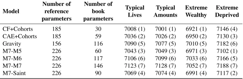
Table 4. Effective number of parameters and AIC for the book part of different

two-population models fitted to the four test books.

Model

Number of reference parameters

Number of book parameters

Typical Lives

Typical Amounts

Extreme Wealthy

Extreme Deprived

CF+Cohorts 185 30 7008 (1) 7001 (1) 6921 (1) 7146 (4)

CAE+Cohorts 185 59 7036 (2) 7026 (2) 6950 (2) 7130 (3)

Gravity 156 116 7090 (5) 7077 (5) 7010 (5) 7182 (6)

M7-M5 226 60 7043 (3) 7049 (3) 6971 (3) 7102 (1)

M7-M6 226 117 7106 (6) 7099 (6) 7033 (6) 7166 (5)

M7-M7 226 146 7123 (7) 7128 (7) 7052 (7) 7188 (7)

M7-Saint 226 90 7069 (4) 7074 (4) 6991 (4) 7117 (2)

parameters such as the Augmented Common Factor model and the Plat+Lee-Carter model.

The graphic testing of the goodness-of-fit of the models leaves us with six potential candidate models for basis risk assessment. These models are: CAE+Cohorts, Gravity, M7-M5, M7-M6, M7-M7, and M7-Saint. The balance between goodness-of-fit and parsimony of these models is investigated in Table 4 where we show the AIC values8for the book part of each model when applied to the four sample schemes, together with the corresponding ranking across models (in brackets). From Table 4 we note the following:

• The CF+Cohorts, which is the simplest model among all the models fitted, tops the AIC ranking for three out of four datasets. However, as noted before, this model is not suitable for basis risk assessment since it assumes that the reference and book populations are perfectly correlated. One may nevertheless consider this model for other applications where the correlation between the populations is not important.

8_{The AIC value is computed asAIC=2}

νB−2LBwhereLBis the Binomial log-likelihood of the book

part of the model under the assumption that the reference population is treated as a known offset andνBis

• Among all other models, the CAE+Cohort and M7-M5 show the best compromise between goodness-of-fit and parsimony, consistently ranking in the top three places and with very similar performance.

• M7-Saint and M7-M7, which have a quadratic age term in the book model, are always outperformed by the M7-M5 model. This suggests that when considering models from the CBD-Family it is necessary to allow for differences in level of mortality and a gradient by age, but that an additional parameter for the curvature by age is not necessary, i.e., it is sufficient to inherit the curvature from the reference population. Thus, we eliminate the M7-M7 and M7-Saint models from our list of candidate models.

• The Gravity model, M7-M6 and M7-M7, which have a book-specific cohort effect, have the worst trade-off between goodness-of-fit and parsimony. This suggests that we should generally reject models with a book cohort effect on grounds of parsimony. However, for the moment we shall retain the Gravity model (two-population APC) which, among models with book-specific cohort effect, shows the best compromise between goodness-of-fit and parsimony. This will enable us to investigate how forecasts levels of uncertainty and hedge effectiveness may be impacted by allowing for a book-specific cohort effect.

6.2.5. Plausibility of forecast central trends and levels of uncertainty

So far, we have shortlisted the CAE+Cohorts, Gravity and M7-M5 based on their theoretical properties, practicality and goodness-of-fit performance. However, the outcome of a basis risk assessment exercise will be strongly driven by the expected level of uncertainty around the central forecast of the demographic and financial quantities underlying the index-based hedge. It is then crucial to check that these models produce reasonable forecast for both single and two-population metrics. This entails judging whether or not the forecast central trajectories and patterns of uncertainty look plausible and are in line with historical variability.

Following Cairns et al. (2011b), we assess this property by examining fan charts of the forecasts produced by the models. Fan charts allow us to examine any distinctive visual feature of the forecasts of the models, as well as the differences between models. Each fan chart presents 95% prediction intervals and depicts the forecast output from the stochastic mortality models by also presenting 80% and 50% prediction intervals.

In producing the model simulations underlying the fan charts, we have considered the following two sources of uncertainty (risk): i) process risk (PR) arising from the possible future trajectories of the time series of the period and cohort indices and ii)

parameter uncertainty(PU) arising from the estimation of the parameters of the model. Process risk is taken into account by simulating trajectories of the period and cohort indices,9while parameter uncertainty is allowed for by using a Binomial adaptation of the residual bootstrapping approach proposed by Koissi et al. (2006).10 We note that due to

9_{To model process risk we use a multivariate adaptation of Algorithm 2 in Haberman and Renshaw (2009)}

without provision for parameter error. We note that Algorithm 2 in Haberman and Renshaw (2009) is itself an adaptation of the prediction interval approach of Cairns et al. (2006).

10_{We note that in adapting the bootstrap we follow Renshaw and Haberman (2008) and solve for the}

the considerable exposure of the England and Wales population, we deliberately ignore parameter uncertainty in the reference population.

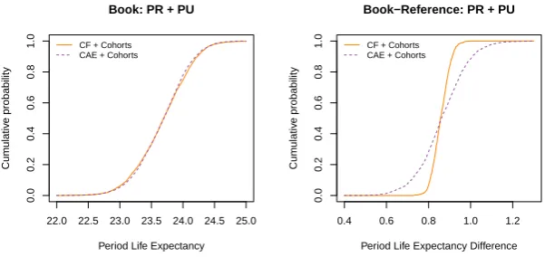
Rather than analysing forecasts of mortality rates, we concentrate on the forecast of life expectancies and survival rates. According to Coughlan et al. (2011), these two aggregate quantities are more appropriate than individual mortality rates for gaining insight into the basis risk associated with longevity hedges. On the one hand, life expectancies and survival rates are more closely related to the hedge effectiveness objective than mortality rates, as, for instance, in a pensioner population life expectancy corresponds to the number of years over which a pension needs to be paid while survival rates correspond to the number of pensioners who are still alive to receive pension. On the other hand, these aggregate metrics smooth out a lot of the noise associated with individual mortality rates.

Figure 5 presents fan charts of 30 year curtailed period life expectancies at age 60,

↑

ei

60,30(t) = 30

∑

h=1

h−1

∏

j=0

(1−qi_60+j,t), i=R,B,

along with fan charts for the value of a cohort survivor index,

Si(65,t) =

t−1

∏

j=0

(1−qi_65+j,2011+j), i=R,B,

for the reference population (i=R) and for the “Extreme Wealthy” test book (i=B). Figure 5 also shows matching fan charts of the difference between the period life expectancies in the book and the reference population, e↑B

60,30(t)− ↑

eR

60,30(t), and of the ratio of the

book and reference population survivor indexes,SB(65,t)/SR(65,t). The survivor index,

Si(65,t),i=R,B, measures the proportion from a group of males aged 65 at the start of 2011 who are still alive at the start of year 2011+t. We note thatSR(65,t)andSB(65,t)

do not involve any forecasts of the cohort effects as the relevant cohort effects,γ₁₉₄₆R and γ₁₉₄₆B in the case of the Gravity model, are known at the start of 2011.

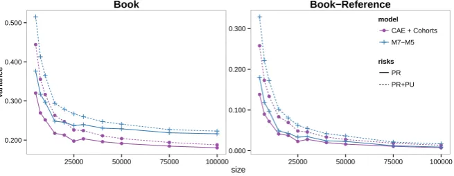
To assist in the assessment of the levels of uncertainty produced by the models, Table 5 presents the forecast variance of period life expectancies in 2020 at age 60,e↑R

60,30(2020)

and↑eB

60,30(2020), while Table 6 presents the forecast variance of the 25 year cohort life

expectancy for someone aged 65 in 2011 in the reference and book populations,

%

ei

65,25(2011) = 25

∑

t=1

Si(65,t) =

25

∑

t=1

t−1

∏

j=0

(1−qi_65+j,2011+j), i=R,B.

From Figure 5 and Tables 5, 6 we can see that:

16 18 20 22 24 26 Reference calendar year Lif e Expectancy

1981 1991 2001 2011 2021 2031

●●●●●● ●●● ●●●● ●●● ●●● ●●● ● ●● ●●● ●● ●●●●●● ●●● ●●●● ●●● ●●● ●●● ● ●● ●●● ●● ●●●●●● ●●● ●●●● ●●● ●●● ●●● ● ●● ●●● ●● ●●●●●● ●●● ●●●● ●●● ●●● ●●● ● ●● ●●● ●●

CF + Cohorts CAE + Cohorts Gravity M7−M5 0.2 0.4 0.6 0.8 1.0 Reference calendar year Sur viv or Inde x

2011 2016 2021 2026 2031 2036 CF + Cohorts

CAE + Cohorts Gravity M7−M5 16 18 20 22 24 26

Book: PR + PU

calendar year

Lif

e Expectancy

1981 1991 2001 2011 2021 2031

●● ●●●● ●●● ●●●●●● ●●●● ●●● ● ●●●● ●● ● ●● ●●●● ●●● ●●●●●● ●●●● ●●● ● ●●●● ●● ● ●● ●●●● ●●● ●●●●●● ●●●● ●●● ● ●●●● ●● ● ●● ●●●● ●●● ●●●●●● ●●●● ●●● ● ●●●● ●● ●

CF + Cohorts CAE + Cohorts Gravity M7−M5 0.2 0.4 0.6 0.8 1.0

Book: PR + PU

calendar year

Sur

viv

or Inde

x

2011 2016 2021 2026 2031 2036 CF + Cohorts

CAE + Cohorts Gravity M7−M5

0.5

1.0

1.5

Book − Reference: PR + PU

calendar year

Lif

e Expectancy Diff

erence

1981 1991 2001 2011 2021 2031

●● ● ●●● ● ● ● ● ● ● ● ● ● ● ●●● ●●●● ● ●● ● ● ● ● ●● ● ●●● ● ● ● ● ● ● ● ● ● ● ●●● ●●●● ● ●● ● ● ● ● ●● ● ●●● ● ● ● ● ● ● ● ● ● ● ●●● ●●●● ● ●● ● ● ● ● ●● ● ●●● ● ● ● ● ● ● ● ● ● ● ●●● ●●●● ● ●● ● ● ● ●

CF + Cohorts CAE + Cohorts Gravity M7−M5 0.95 1.05 1.15 1.25

Book / Reference: PR + PU

calendar year

Sur

viv

or Inde

x Ratio

2011 2016 2021 2026 2031 2036 CF + Cohorts

CAE + Cohorts Gravity M7−M5

Figure 5.Fan charts of 30 year period curtailed life expectancy at age 60,

↑

ei

60,30(t),i=R,B, and of the cohort survivor index,S

i_{(65,t),i=R,B, for the England and} Wales reference population and the “Extreme Wealthy” book using different mortality models.