A Zero-attracting Quaternion-valued Least Mean Square Algorithm for Sparse System Identification

This is a repository copy of

A Zero-attracting Quaternion-valued Least Mean Square

Algorithm for Sparse System Identification

.

White Rose Research Online URL for this paper:

http://eprints.whiterose.ac.uk/94837/

Version: Accepted Version

Proceedings Paper:

Jiang, M.D., Liu, W. and Li, Y. (2014) A Zero-attracting Quaternion-valued Least Mean

Square Algorithm for Sparse System Identification. In: 9th International Symposium on

Communication Systems, Networks & Digital Signal Processing (CSNDSP), 2014.

International Symposium on Communication Systems, Networks and Digital Signal

Processing (CSNDSP), 23-25 Jul 2014, Manchester, UK. IEEE .

https://doi.org/10.1109/CSNDSP.2014.6923898

[email protected] https://eprints.whiterose.ac.uk/

Reuse

Unless indicated otherwise, fulltext items are protected by copyright with all rights reserved. The copyright exception in section 29 of the Copyright, Designs and Patents Act 1988 allows the making of a single copy solely for the purpose of non-commercial research or private study within the limits of fair dealing. The publisher or other rights-holder may allow further reproduction and re-use of this version - refer to the White Rose Research Online record for this item. Where records identify the publisher as the copyright holder, users can verify any specific terms of use on the publisher’s website.

Takedown

If you consider content in White Rose Research Online to be in breach of UK law, please notify us by

arXiv:1406.5721v1 [math.NA] 22 Jun 2014

A Zero-attracting Quaternion-valued Least Mean

Square Algorithm for Sparse System Identification

Mengdi Jiang, Wei Liu

Communications Research Group

Department of Electronic and Electrical Engineering University of Sheffield, UK

{mjiang3, w.liu}@sheffield.ac.uk

Yi Li

School of Mathematics and Statistics University of Sheffield, S3 7RH UK

[email protected]

Abstract—Recently, quaternion-valued signal processing has

received more and more attention. In this paper, the quaternion-valued sparse system identification problem is studied for the first time and a zero-attracting quaternion-valued least mean square (LMS) algorithm is derived by considering thel_{1 norm of the}

quaternion-valued adaptive weight vector. By incorporating the sparsity information of the system into the update process, a faster convergence speed is achieved, as verified by simulation results.

Keywords: quaternion; sparsity; system identification; adap-tive filtering; LMS algorithm.

I. INTRODUCTION

In adaptive filtering [1], there is a class of algorithms specifically designed for sparse system identification, where the unknown system only has a few large coefficients while the remaining ones have a very small amplitude so that they can be ignored without significant effect on the overall performance of the system. A good example of them is the zero-attracting least mean square (ZA-LMS) algorithm proposed in [2]. This algorithm can achieve a higher convergence speed, and meanwhile, reduce the steady state excess mean square error (MSE). Compared to the classic LMS algorithm [3], the ZA-LMS algorithm introduces an l1 norm in its cost function, which modifies the weight vector update equation with a zero attractor term.

Recently, the hypercomplex concepts have been introduced to solve problems related to three or four-dimensional sig-nals [4], such as vector-sensor array signal processing [5], [6], [7], color image processing [8] and wind profile prediction [9], [10]. As quaternion-valued algorithms can be regarded as an extension of the complex-valued ones, the adaptive filtering algorithms in complex domain could be extended to the quaternion domain as well, such as the quaternion-valued LMS (QLMS) algorithm in [11].

This work is partially funded by National Grid, UK and will appear in the Proc. of the 9th International Symposium on Communication Systems, Networks and Digital Signal Processing (CSNDSP), Manchester, UK, July 2014 (submitted in March 2014 and accepted on 18 April 2014).

In this paper, we propose a novel quaternion-valued adaptive algorithm with a sparsity constraint, which is called zero-attracting QLMS (ZA-QLMS) algorithm. The additional con-straint is formulated based on the l1 norm. Both the QLMS and ZA-QLMS algorithms can identify an unknown sparse system effectively. However, a better performance in terms of convergence speed is achieved by the latter one.

This paper is organized as follows. A review of basic operations in the quaternion domain is provided in Section II to facilitate the following derivation of the ZA-QLMS algorithm. The proposed ZA-QLMS algorithm is derived in Section III. Simulation results are given in Section IV, and conclusions are drawn in Section V.

II. QUATERNION-VALUEDADAPTIVEFILTERING

A. Basics of Quaternion

Quaternion is a non-commutative extension of the complex number, and normally a quaternion consists of one real part and three imaginary parts, denoted by subscripts a, b, c and

d, respectively.

For a quaternion numberq, it can be described as

q=qa+ (qbi+qcj+qdk), (1)

where qa, qb, qc, and qd are real-valued [12], [13]. For a quaternion, when its real part is zero, it becomes a pure quaternion. In this paper, we consider the conjugate operator ofqas q∗_{=qa−qbi−qcj−qdk. The three imaginary units}

i,j, andk satisfy

ij=k, jk=i, ki=j, ijk=i2

=j2

=k2

=−1. (2)

As a quaternion has the noncommutativity property, in multiplication, the exchange of any two elements in their order will give a different result. For example, we have ji =−ij

B. Differentiation with Respect to a Quaternion-valued Vector

To derive the quaternion-valued adaptive algorithm, the starting point is the general operation of differentiation with respect to a quaternion-valued vector.

At first, we need to give the definition of differentiation with respect to a quaternionq and its conjugate q∗_{. Assume}

thatf(q)is a function of the quaternion variableq, which is expressed as

f(q) =fa+fbi+fcj+fdk (3)

wheref(q)is in general quaternion-valued. The definition of

df(q)

dq can be expressed as [14], [11]

df(q) dq = 1 4( ∂f(q) ∂qa

−∂f(q)

∂qb

i−∂f(q)

∂qc

j−∂f(q)

∂qd

k). (4)

The derivative off(q)with respect toq∗ _{can be defined in}

a similar way

df(q) dq∗ =

1 4(

∂f(q) ∂qa

+∂f(q) ∂qb

i+∂f(q) ∂qc

j+∂f(q) ∂qd

k). (5)

With this definition, we can easily obtain

∂q ∂q = 1,

∂q ∂q∗ =−

1

2 . (6)

Some product rules can be obtained from above formula-tions, such as the differentiation of quaternion-valued functions to real variables.

Supposef(q)andg(q)are two quaternion-valued functions of the quaternion variableq, andqa is the real variable. Then we can have the following result

∂f(q)g(q) ∂qa

= ∂

∂qa

(fa+ifb+jfc+kfd)g

= ∂fag ∂qa

+i∂fbg ∂qa

+j∂fcg ∂qa

+k∂fdg ∂qa

= (fa

∂g ∂qa

+∂fa ∂qa

g) +i(fb

∂g ∂qa

+∂fb ∂qa

g)

+j(fc

∂g ∂qa

+∂fc ∂qa

g) +k(fd

∂g ∂qa

+∂fd ∂qa

g)

= (fa+ifb+jfc+kfd)

∂g ∂qa

+(∂fa ∂qa

+i∂fb ∂qa

+j∂fc ∂qa

+k∂fd ∂qa

)g

= f(q)∂g(q) ∂qa

+∂f(q) ∂qa

g(q) (7)

When the quaternion variableqis replaced by a quaternion-valued vector w, given by

w= [w1 w2 · · · wM] T

(8)

where wm = am+bmi+cmj +dmk, m = 1, ..., M, the differentiation of the functionf(w)with respect to the vector

w can be derived using a combination of (4) straightforwardly in the following

∂f ∂w =

1 4           ∂f ∂a0 − ∂f ∂b0

i− ∂f

∂c0

j− ∂f

∂d0

k ∂f

∂a1 −i∂f

∂b1

i− ∂f

∂c1

j− ∂f

∂d1

k

.. .

∂f ∂aM₋1

− ∂f

∂bM₋1

i− ∂f

∂cM₋1

j− ∂f

∂dM₋1

k           (9)

Similarly, we define ∂f

∂w∗ as

∂f ∂w∗ =

1 4           ∂f ∂a0 + ∂f ∂b0

i+ ∂f ∂c0

j+ ∂f ∂d0 k ∂f ∂a1 + ∂f ∂b1

i+ ∂f ∂c1

j+ ∂f ∂d1

k

.. .

∂f ∂aM₋1

+ ∂f

∂bM₋1

i+ ∂f ∂cM₋1

j+ ∂f ∂dM₋1

k           (10)

Obviously, whenM = 1, (9) and (10) are reduced to (4) and (5), respectively.

III. THEZERO-ATTRACTINGQLMS (ZA-QLMS) ALGORITHM

To improve the performance of the LMS algorithm for sparse system identification, the ZA-QLMS algorithm is de-rived in this section. To achieve this, similar to [2], in the cost function, we add anl1 norm penalty term for the quaternion-valued weight vector w[n].

For a standard adaptive filter, the outputy[n]and errore[n]

can be expressed as

y[n] = wT[n]x[n] (11)

e[n] = d[n]−wT[n]x[n], (12)

where w[n] is the adaptive weight vector with a length ofL,

d[n]is the reference signal, x[n] = [x[n−1],· · ·, x[n−L]]T is the input sample vector, and {·}T

denotes the transpose operation. Moreover, the conjugate form e∗_{[n] of the error}

signale[n] is given by

e∗_{[n] =d}∗_[n]−xH

[n]w∗_{[n], (13)}

Our proposed cost function with a zero attractor term is given by

J0[n] =e[n]e∗[n] +γkw[n]k1, (14) whereγ is a small constant.

The gradient of the above cost function with respect to w∗_{[n] and w[n] can be respectively expressed as}

∇w∗J0[n] =

∂J0[n]

∂w∗ (15)

and

∇wJ0[n] =

∂J0[n]

From [14], [15], we know that the conjugate gradient gives the maximum steepness direction for the optimization surface. Therefore, the conjugate gradient ∇w∗J0[n] will be used to derive the update of the coefficient weight vector.

Expanding the cost function, we obtain

J0[n] = e[n]e∗[n] +γkw[n]k₁

= d[n]d∗_[n]−d[n]xH

[n]w∗_[n]−wT

[n]x[n]d∗_[n]

+wT[n]x[n]xH[n]w∗_{[n] +γkw[n]k}

1. (17)

Furthermore,

∂J0[n]

∂w∗ =

∂(e[n]e∗_{[n] +γkw[n]k}

1)

∂w∗

= ∂

∂w∗(d[n]d

∗_[n]−d[n]xH

[n]w∗_[n]

−wT[n]x[n]d∗_{[n] +w}T_[n]x[n]xH_[n]w∗_[n])

+∂(γkw[n]k1)

∂w∗ . (18)

Details of the derivation process for the gradient are shown in the following

∂(d[n]d∗_[n])

∂w∗_[n] = 0 (19)

∂(d[n]xH[n]w∗_[n])

∂w∗_[n] =d[n]x

∗_{[n] (20)}

∂(wT[n]x[n]d∗_[n])

∂w∗_[n] =−

1 2d[n]x

∗_{[n] (21)}

∂(wT[n]x[n]xH[n]w∗_[n])

∂w∗_[n] =

1 2w

T

[n]x[n]x∗_{[n]. (22)}

Moreover, the last part of the gradient of cost function is given by

∂(γkw[n]k1)

∂w∗ =

1

4γ·sgn(w[n]), (23)

where the symbolsgnis a component-wise sign function that is defined as [2]

sgn(x) =

(

x/|x| x6= 0

0 x= 0

Combining the above results, the final gradient can be obtained as follows

∇w∗J0[n] =−

1 2e[n]x

∗_{[n] +} 1

4γ·sgn(w[n]). (24)

With the general update equation for the weight vector

w[n+ 1] =w[n]−µ∇w∗J0[n], (25)

where µ is the step size, we arrive at the following update equation for the proposed ZA-QLMS algorithm

w[n+ 1] =w[n] +µ(e[n]x∗_{[n])−ρ·sgn(w[n]), (26)}

where ρ = µγ. The last term represents the zero attractor, which enforces the near-zero coefficients to zero and therefore

accelerates the convergence process when majority of the system coefficients are nearly zero in a sparse system.

Note that equation (26) will be reduced to the normal QLMS algorithm without the zero attractor term, given by [11]

w[n+ 1] =w[n] +µ(e[n]x∗_{[n]). (27)}

IV. SIMULATIONRESULTS

In this part, simulations are performed for sparse system identification using the proposed algorithm in comparison with the QLMS algorithm. Two different sparse systems are considered corresponding to Scenario One and Scenario Two in the following. The input signal to the adaptive filter is colored and generated by passing a quaternion-valued white gaussian signal through a randomly generated filter. The noise part is quaternion-valued white Gaussian and added to the output of the unknown sparse system, with a 30dB signal to noise ratio (SNR) for both scenarios.

A. Scenario One

For the first scenario, the parameters are: the step sizeµis

3×10−7

; the unknown sparse FIR filter lengthL is32, with

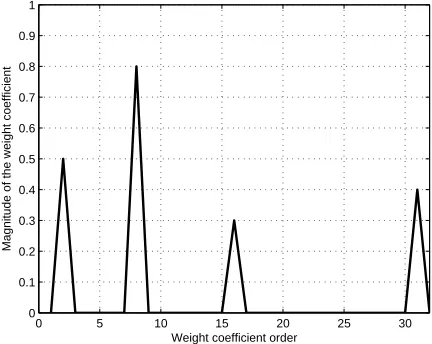
4non-zero coefficients at the 2nd, 8th, 16th and 31st taps, and its magnitude of the impulse response is shown in Fig. 1; the coefficient of the zero attractor ρ is 5×10−7

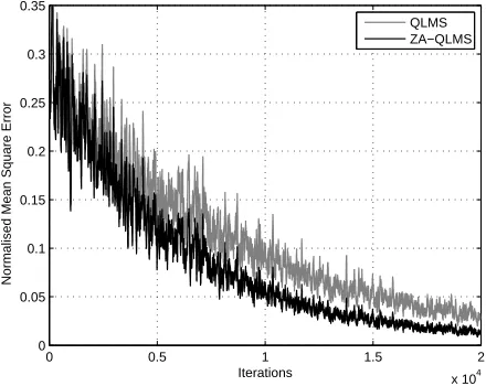
. The learning curve obtained by averaging 100 runs of the corresponding algorithm is given in Fig. 2, where we can see that the ZA-QLMS algorithm has achieved a faster convergence speed than the QLMS algorithm when they both reach a similar steady state.

0 5 10 15 20 25 30

0 0.1 0.2 0.3 0.4 0.5 0.6 0.7 0.8 0.9 1

Weight coefficient order

Magnitude of the weight coefficient

Fig. 1. Magnitude of the impulse response of the sparse system.

B. Scenario Two

0 0.5 1 1.5 2

x 104 0

0.05 0.1 0.15 0.2 0.25 0.3 0.35

Iterations

Normalised Mean Square Error

QLMS ZA−QLMS

Fig. 2. Learning curves for the first scenario.

is 2×10−7

and the value of ρ is 2×10−7

. The results are shown in Fig. 3. Again we see that the ZA-QLMS algorithm has a faster convergence speed and has even converged to a lower steady state error in this specific scenario.

0 0.5 1 1.5 2

x 104 0

0.05 0.1 0.15 0.2 0.25 0.3 0.35

Iterations

Normalised Mean Square Error

QLMS ZA−QLMS

Fig. 3. Learning Curves for the second scenario.

V. CONCLUSION

In this paper, a quaternion-valued adaptive algorithm has been proposed for more efficient identification of unknown sparse systems. It is derived by introducing anl1penalty term in the original cost function and the resultant zero-attracting quaternion-valued LMS algorithm can achieve a faster con-vergence rate by incorporating the sparsity information of the system into the update process. Simulation results have been provided to show the effectiveness of the new algorithm.

REFERENCES

[1] S. Haykin, Adaptive Filter Theory, Prentice Hall, Englewood Cliffs, New York, 3rd edition, 1996.

[2] Yilun Chen, Yuantao Gu, and Alfred O Hero, “Sparse LMS for system identification,” in Acoustics, Speech and Signal Processing, 2009. ICASSP 2009. IEEE International Conference on. IEEE, 2009, pp. 3125–3128.

[3] B. Widrow, J. McCool, and M. Ball, “The Complex LMS Algorithm,” Proceedings of the IEEE, vol. 63, pp. 719–720, August 1975. [4] N. Le Bihan and J. Mars, “Singular value decomposition of quaternion

matrices: a new tool for vector-sensor signal processing,” Signal Processing, vol. 84, no. 7, pp. 1177–1199, 2004.

[5] X.R. Zhang, W. Liu, Y.G. Xu, and Z.W. Liu, “Quaternion-based worst case constrained beamformer based on electromagnetic vectoe-sensor arrays,” in Proc. IEEE International Conference on Acoustics, Speech, and Signal Processing, Vancouver, Canada, May 2013, pp. 4149–6153. [6] X. R. Zhang, W. Liu, Y. G. Xu, and Z. W. Liu, “Quaternion-valued robust adaptive beamformer for electromagnetic vector-sensor arrays with worst-case constraint,” Signal Processing, vol. 104, pp. 274–283, November 2014.

[7] M. B. Hawes and W. Liu, “A quaternion-valued reweighted minimisation approach to sparse vector sensor array design,” in Proc. of the International Conference on Digital Signal Processing, Hong Kong, August 2014.

[8] S.C. Pe and C.M. Cheng, “Color image processing by using binary quaternion-moment-preserving thresholding technique,” Image Process-ing, IEEE Transactions on, vol. 8, no. 5, pp. 614–628, 1999. [9] Clive Cheong Took and Danilo P Mandic, “The quaternion LMS

algorithm for adaptive filtering of hypercomplex processes,” IEEE Transactions on Signal Processing, vol. 57, no. 4, pp. 1316–1327, 2009. [10] M. D. Jiang, W. Liu, Y. Li, and X. R. Zhang, “Frequency-domain quaternion-valued adaptive filtering and its application to wind profile prediction,” in Proc. of the IEEE TENCON Conference, Xi’an, China, October 2013.

[11] M. D. Jiang, W. Liu, and Y. Li, “A general quaternion-valued gradient operator and its applications to computational fluid dynamics and adaptive beamforming,” in Proc. of the International Conference on Digital Signal Processing, Hong Kong, August 2014.

[12] William Rowan Hamilton, Elements of quaternions, Longmans, Green, & co., 1866.

[13] I. Kantor, A.S. Solodovnikov, and Abe Shenitzer, Hypercomplex numbers: an elementary introduction to algebras, Springer Verlag, New York, 1989.

[14] Danilo P Mandic, Cyrus Jahanchahi, and Clive Cheong Took, “A quater-nion gradient operator and its applications,” IEEE Signal Processing Letters, vol. 18, no. 1, pp. 47–50, 2011.